如果你也在 怎样代写博弈论Game theory 这个学科遇到相关的难题,请随时右上角联系我们的24/7代写客服。博弈论Game theory在20世纪50年代被许多学者广泛地发展。它在20世纪70年代被明确地应用于进化论,尽管类似的发展至少可以追溯到20世纪30年代。博弈论已被广泛认为是许多领域的重要工具。截至2020年,随着诺贝尔经济学纪念奖被授予博弈理论家保罗-米尔格伦和罗伯特-B-威尔逊,已有15位博弈理论家获得了诺贝尔经济学奖。约翰-梅纳德-史密斯因其对进化博弈论的应用而被授予克拉福德奖。
博弈论Game theory是对理性主体之间战略互动的数学模型的研究。它在社会科学的所有领域,以及逻辑学、系统科学和计算机科学中都有应用。最初,它针对的是两人的零和博弈,其中每个参与者的收益或损失都与其他参与者的收益或损失完全平衡。在21世纪,博弈论适用于广泛的行为关系;它现在是人类、动物以及计算机的逻辑决策科学的一个总称。
statistics-lab™ 为您的留学生涯保驾护航 在代写博弈论Game Theory方面已经树立了自己的口碑, 保证靠谱, 高质且原创的统计Statistics代写服务。我们的专家在代写博弈论Game Theory代写方面经验极为丰富,各种代写博弈论Game Theory相关的作业也就用不着说。

经济代写|博弈论代写Game Theory代考|Ultimatum Games: Power to the Proposer
The ultimatum bargaining game is perhaps the simplest of bargaining models. In the example presented in Chapter 14 (see Figure 14.5), a buyer and a seller negotiate the price of a painting. The seller offers a price and then the buyer accepts or rejects it, ending the game. Because the painting is worth $\$ 100$ to the buyer and nothing to the seller, trade will generate a surplus of $\$ 100$. The price determines how this surplus is divided between the buyer and the seller; that is, it describes the terms of trade. From the Guided Exercise of Chapter 15 , you have already seen that there is a subgame perfect equilibrium of this game in which trade takes place at a price of 100 , meaning that the seller gets the entire surplus. In this section, I expand the analysis to show that this equilibrium is unique.
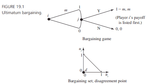
It will be helpful to study the ultimatum bargaining game in the abstract setting in which the surplus is normalized to 1 . This normalization helps us to concentrate on the players’ shares of the monetary surplus; for example, if player 1 obtains $1 / 4$, then it means that player 1 gets 25 percent of the surplus. As discussed in Chapter 18 , we assume transferable utility so that the price divides the surplus in a linear fashion; thus, if one player gets $m$, then the other gets $1-m$. It will also be helpful to name the players $i$ and $j$, allowing us to put either player 1 or player 2 into the role of making the offer. This standard ultimatum game is pictured in Figure 19.1.
Also pictured are the bargaining set and the disagreement point corresponding to this game. The disagreement point is $(0,0)$ because this payoff occurs when the responder rejects the proposer’s offer.
To find the subgame perfect equilibrium of the ultimatum game, begin by observing that the game has an infinite number of subgames. In particular, every decision node for player $j$ initiates a subgame (that ends following his decision). This should be obvious because player $j$ observes the offer of player $i$; all information sets consist of single nodes. Consider the subgame following any particular offer of $m$ by player $i$, where $m>0$. If player $j$ accepts the offer, he obtains $m$. If he rejects the offer, then he gets 0 . Therefore, player $j$ ‘s best action is to accept. Only when $m=0$ can rejection be an optimal response for player $j$, and in this case acceptance also is optimal (because player $j$ is indifferent between the two actions). The analysis thus indicates that player $j$ has only two sequentially rational strategies: $\left(s_j^*\right)$ accept all offers, and $\left(\hat{s}_j\right)$ accept all offers of $m>0$ and reject the offer of $m=0$. These are the only strategies that specify a Nash equilibrium for each of the proper subgames.
经济代写|博弈论代写Game Theory代考|Two-Period, Alternating-Offer Games: Power to the Patient
The ultimatum game is instructive and applicable, but it is too simplistic a model of most real-world negotiation. Bargaining generally follows a more intricate process in reality. The theory can be expanded in many ways, perhaps the most obvious of which is to explicitly model multiple offers and counteroffers by the parties over time. In fact, in many real settings, the sides alternate making offers until one is accepted. For example, real estate agents routinely force home sales into the following procedure: the seller posts a price, the prospective buyer makes an offer that differs from the seller’s asking price, the seller makes a counteroffer, and so forth.
Offers and counteroffers take time. In home sales, one party may wait a week or more for an offer to be considered and a counteroffer returned. “Time is money,” an agent may say between utterances of the “location, location, location” mantra. In fact, the agent is correct to the extent that people are impatient or forego productive opportunities during each day spent in negotiation. Most people are impatient to some degree. Most people prefer not to endure protracted negotiation procedures. Most people discount the future relative to the present.
How a person discounts the future may affect his or her bargaining position. It seems reasonable to expect that a very patient bargainer-or someone who has nothing else to do and nowhere else to go-should be able to win a greater share of the surplus than should an impatient one. To incorporate discounting into game-theoretic models, we use the notion of a discount factor. A discount factor $\delta_i$ for player $i$ is a number used to deflate a payoff received tomorrow so that it can be compared with a payoff received today.
To make sense of this idea, fix a length of time that we call the period length. For simplicity, suppose that a period corresponds to 1 week. If given the choice, most people would prefer receiving $x$ dollars today (in the current period) rather than being assured of receiving $x$ in one week (in the next period). People exhibit this preference because people are generally impatient, perhaps because they would like the opportunity to spend money earlier rather than later. In the least, a person could take the $x$ dollars received today and deposit it in a bank account to be withdrawn next week with interest.
博弈论代考
经济代写|博弈论代写Game Theory代考|Ultimatum Games: Power to the Proposer
最后通牒议价博弈也许是最简单的议价模型。在第14章给出的例子中(见图14.5),一个买家和一个卖家协商一幅画的价格。卖家给出一个价格,然后买家接受或拒绝,游戏结束。因为这幅画对买家来说价值$\$ 100$,对卖家来说一文不值,所以交易将产生$\$ 100$的盈余。价格决定了这个剩余部分如何在买方和卖方之间分配;也就是说,它描述了贸易条件。从第15章的指导练习中,你已经看到了这个博弈的一个子博弈完美均衡,在这个博弈中,交易以100的价格进行,这意味着卖方获得了全部剩余。在本节中,我将展开分析,以证明这种均衡是唯一的。
在盈余归一化为1的抽象情况下,研究最后通牒议价博弈是有益的。这种正常化有助于我们关注参与者在货币盈余中所占的份额;例如,参与人1获得$1 / 4$,则意味着参与人1获得剩余的25%。正如第18章所讨论的,我们假设可转移效用,因此价格以线性方式划分剩余;因此,如果一个玩家得到$m$,那么另一个玩家得到$1-m$。将参与者命名为$i$和$j$也很有帮助,允许我们将参与者1或参与者2置于提出报价的角色中。这个标准的最后通牒游戏如图19.1所示。
图中还有与这个游戏相对应的讨价还价集和分歧点。分歧点是$(0,0)$,因为当响应者拒绝提议者的提议时,就会出现这种回报。
要找到最后通牒博弈的子博弈完美均衡,首先要观察这个博弈有无限多个子博弈。特别是,玩家$j$的每个决策节点都会启动一个子游戏(在他的决策之后结束)。这应该是显而易见的,因为玩家$j$会观察玩家$i$的提议;所有信息集都由单个节点组成。考虑玩家$i$提供$m$后的子游戏,其中$m>0$。如果玩家$j$接受报价,他将获得$m$。如果他拒绝这个提议,那么他得0。因此,玩家$j$的最佳行动是接受。只有当$m=0$拒绝才是玩家$j$的最佳反应,在这种情况下接受也是最优的(因为玩家$j$在两种行为之间是无所谓的)。分析表明,参与人$j$只有两个顺序理性策略:$\left(s_j^*\right)$接受所有条件,$\left(\hat{s}_j\right)$接受$m>0$的所有条件,拒绝$m=0$的条件。这是为每个适当的子博弈指定纳什均衡的唯一策略。
经济代写|博弈论代写Game Theory代考|Two-Period, Alternating-Offer Games: Power to the Patient
最后通牒游戏具有启发性和适用性,但对于大多数现实世界的谈判来说,它过于简单化了。在现实中,讨价还价通常遵循一个更复杂的过程。该理论可以在许多方面得到扩展,其中最明显的可能是明确地模拟各方在一段时间内的多次要约和还价。事实上,在许多现实情况下,双方轮流提出条件,直到其中一方被接受。例如,房地产经纪人通常迫使房屋销售进入以下程序:卖方发布价格,潜在买家提出与卖方要价不同的报价,卖方提出还价,等等。
报价和还价都需要时间。在房屋销售中,一方可能会等待一周或更长的时间,等待报价被考虑,并收到还价。“时间就是金钱,”代理人可能会在“地点,地点,地点”的口头禅中说。事实上,在某种程度上,代理人是正确的,人们在每天的谈判中都不耐烦或放弃了生产机会。大多数人在某种程度上都没有耐心。大多数人不愿意忍受冗长的谈判过程。相对于现在,大多数人低估了未来。
一个人如何贴现未来可能会影响他或她的议价地位。似乎有理由认为,一个非常有耐心的讨价还价者——或者一个无事可做、无处可去的人——应该能够比一个没有耐心的人赢得更多的剩余份额。为了将折扣纳入博弈论模型,我们使用了折扣因子的概念。对于参与人i来说,折现系数是一个用来减少明天收到的收益的数字,以便与今天收到的收益进行比较。
为了理解这个概念,固定一个时间长度,我们称之为周期长度。为简单起见,假设一个周期对应于1周。如果可以选择,大多数人宁愿今天(在当前时期)得到x美元,也不愿在一周(在下一时期)得到x美元。人们表现出这种偏好是因为人们通常没有耐心,也许是因为他们希望有机会早点花钱而不是晚点。至少,一个人可以把今天收到的x美元存入一个银行账户,下周取出来,连本带利。

统计代写请认准statistics-lab™. statistics-lab™为您的留学生涯保驾护航。
金融工程代写
金融工程是使用数学技术来解决金融问题。金融工程使用计算机科学、统计学、经济学和应用数学领域的工具和知识来解决当前的金融问题,以及设计新的和创新的金融产品。
非参数统计代写
非参数统计指的是一种统计方法,其中不假设数据来自于由少数参数决定的规定模型;这种模型的例子包括正态分布模型和线性回归模型。
广义线性模型代考
广义线性模型(GLM)归属统计学领域,是一种应用灵活的线性回归模型。该模型允许因变量的偏差分布有除了正态分布之外的其它分布。
术语 广义线性模型(GLM)通常是指给定连续和/或分类预测因素的连续响应变量的常规线性回归模型。它包括多元线性回归,以及方差分析和方差分析(仅含固定效应)。
有限元方法代写
有限元方法(FEM)是一种流行的方法,用于数值解决工程和数学建模中出现的微分方程。典型的问题领域包括结构分析、传热、流体流动、质量运输和电磁势等传统领域。
有限元是一种通用的数值方法,用于解决两个或三个空间变量的偏微分方程(即一些边界值问题)。为了解决一个问题,有限元将一个大系统细分为更小、更简单的部分,称为有限元。这是通过在空间维度上的特定空间离散化来实现的,它是通过构建对象的网格来实现的:用于求解的数值域,它有有限数量的点。边界值问题的有限元方法表述最终导致一个代数方程组。该方法在域上对未知函数进行逼近。[1] 然后将模拟这些有限元的简单方程组合成一个更大的方程系统,以模拟整个问题。然后,有限元通过变化微积分使相关的误差函数最小化来逼近一个解决方案。
tatistics-lab作为专业的留学生服务机构,多年来已为美国、英国、加拿大、澳洲等留学热门地的学生提供专业的学术服务,包括但不限于Essay代写,Assignment代写,Dissertation代写,Report代写,小组作业代写,Proposal代写,Paper代写,Presentation代写,计算机作业代写,论文修改和润色,网课代做,exam代考等等。写作范围涵盖高中,本科,研究生等海外留学全阶段,辐射金融,经济学,会计学,审计学,管理学等全球99%专业科目。写作团队既有专业英语母语作者,也有海外名校硕博留学生,每位写作老师都拥有过硬的语言能力,专业的学科背景和学术写作经验。我们承诺100%原创,100%专业,100%准时,100%满意。
随机分析代写
随机微积分是数学的一个分支,对随机过程进行操作。它允许为随机过程的积分定义一个关于随机过程的一致的积分理论。这个领域是由日本数学家伊藤清在第二次世界大战期间创建并开始的。
时间序列分析代写
随机过程,是依赖于参数的一组随机变量的全体,参数通常是时间。 随机变量是随机现象的数量表现,其时间序列是一组按照时间发生先后顺序进行排列的数据点序列。通常一组时间序列的时间间隔为一恒定值(如1秒,5分钟,12小时,7天,1年),因此时间序列可以作为离散时间数据进行分析处理。研究时间序列数据的意义在于现实中,往往需要研究某个事物其随时间发展变化的规律。这就需要通过研究该事物过去发展的历史记录,以得到其自身发展的规律。
回归分析代写
多元回归分析渐进(Multiple Regression Analysis Asymptotics)属于计量经济学领域,主要是一种数学上的统计分析方法,可以分析复杂情况下各影响因素的数学关系,在自然科学、社会和经济学等多个领域内应用广泛。
MATLAB代写
MATLAB 是一种用于技术计算的高性能语言。它将计算、可视化和编程集成在一个易于使用的环境中,其中问题和解决方案以熟悉的数学符号表示。典型用途包括:数学和计算算法开发建模、仿真和原型制作数据分析、探索和可视化科学和工程图形应用程序开发,包括图形用户界面构建MATLAB 是一个交互式系统,其基本数据元素是一个不需要维度的数组。这使您可以解决许多技术计算问题,尤其是那些具有矩阵和向量公式的问题,而只需用 C 或 Fortran 等标量非交互式语言编写程序所需的时间的一小部分。MATLAB 名称代表矩阵实验室。MATLAB 最初的编写目的是提供对由 LINPACK 和 EISPACK 项目开发的矩阵软件的轻松访问,这两个项目共同代表了矩阵计算软件的最新技术。MATLAB 经过多年的发展,得到了许多用户的投入。在大学环境中,它是数学、工程和科学入门和高级课程的标准教学工具。在工业领域,MATLAB 是高效研究、开发和分析的首选工具。MATLAB 具有一系列称为工具箱的特定于应用程序的解决方案。对于大多数 MATLAB 用户来说非常重要,工具箱允许您学习和应用专业技术。工具箱是 MATLAB 函数(M 文件)的综合集合,可扩展 MATLAB 环境以解决特定类别的问题。可用工具箱的领域包括信号处理、控制系统、神经网络、模糊逻辑、小波、仿真等。