如果你也在 怎样代写信息论information theory 这个学科遇到相关的难题,请随时右上角联系我们的24/7代写客服。信息论information theory回答了通信理论中的两个基本问题:什么是最终的数据压缩(答案:熵$H$),什么是通信的最终传输速率(答案:信道容量$C$)。由于这个原因,一些人认为信息论是通信理论的一个子集。我们认为它远不止于此。
信息论information theory在统计物理学(热力学)、计算机科学(柯尔莫哥洛夫复杂性或算法复杂性)、统计推断(奥卡姆剃刀:“最简单的解释是最好的”)以及概率和统计学(最优假设检验和估计的误差指数)方面都做出了根本性的贡献。
statistics-lab™ 为您的留学生涯保驾护航 在代写信息论information theory方面已经树立了自己的口碑, 保证靠谱, 高质且原创的统计Statistics代写服务。我们的专家在代写信息论information theory代写方面经验极为丰富,各种代写信息论information theory相关的作业也就用不着说。

数学代写|信息论代写information theory代考|The Forth Step: The SMI of Locations and Momenta
of N Independent Particles in a Box of Volume V.
Adding a Correction Due to Indistinguishability
of the Particles
The final step is to proceed from a single particle in a box, to $N$ independent particles in a box of volume $V$, Fig. 2.4.
We say that we know the microstate of the particle, when we know the location $(x, y, z)$, and the momentum $\left(p_x, p_y, p_z\right)$ of one particle within the box. For a system of $N$ independent particles in a box, we can write the SMI of the system as $N$ times the SMI of one particle, i.e., we write:
$$
\mathrm{SMI}(N \text { independent particles })=N \times \mathrm{SMI} \text { (one particle) }
$$
This is the SMI for $N$ independent particles. In reality, there could be correlation among the microstates of all the particles. We shall mention here correlations due to the indistinguishability of the particles, and correlations is due to intermolecular interactions among all the particles. We shall discuss these two sources of correlation separately. Recall that the microstate of a single particle includes the location and the momentum of that particle. Let us focus on the location of one particle in a box of volume $V$. We write the locational SMI as:
$$
H_{\max }(\text { location })=\log V
$$
For $N$ independent particles, we write the locational SMI as:
$$
H_{\max } \text { (locations of N particles) }=\sum_{i=1}^N H_{\max }(\text { one particle })
$$
Since in reality, the particles are indistinguishable, we must correct Eq. (2.22). We define the mutual information corresponding to the correlation between the particles as:
$$
I(1 ; 2 ; \ldots ; N)=\ln N !
$$
Hence, instead of (2.22), for the SMI of $N$ indistinguishable particles, will write:
$$
H(\text { Nparticles })=\sum_{i=1}^N H(\text { oneparticle })-\ln N !
$$
A detailed justification for introducing $\ln N$ ! as a correction due to indistinguishability of the particle is discussed in Sect. 5.2 of Ben-Naim [1]. Here we write the final result for the SMI of $N$ indistinguishable (but non-interacting) particles as:
$$
H(N \text { indistinguishable particles })=N \log V\left(\frac{2 \pi m e k_B T}{h^2}\right)^{3 / 2}-\log N !
$$
数学代写|信息论代写information theory代考|The Entropy of a System of Interacting Particles. Correlations Due to Intermolecular Interactions
In this section we derive the most general relationship between the SMI (or the entropy) of a system of interacting particles, and the corresponding mutual information (MI). Later on in this chapter we shall apply this general result to some specific cases. The implication of this result is very important in interpreting the concept of entropy in terms of SMI. In other words, the “informational interpretation” of entropy is effectively extended for all systems of interacting particles at equilibrium.
We start with some basic concepts from classical statistical mechanics [7]. The classical canonical partition function (PF) of a system characterized by the variable $T, V, N$, is:
$$
Q(T, V, N)=\frac{Z_N}{N ! \Lambda^{3 N}}
$$
where $\Lambda^3$ is called the momentum partition function (or the de Broglie wavelength), and $Z_N$ is the configurational PF of the system”
$$
Z_N=\int \cdots \int d R^N \exp \left[-\beta U_N\left(R^N\right)\right]
$$
Here, $U_N\left(R^N\right)$ is the total interaction energy among the $N$ particles at a configuration $R^N=R_1, \cdots, R_N$. Statistical thermodynamics provides the probability density for finding the particles at a specific configuration $R^N=R_1, \cdots, R_N$, which is:
$$
P\left(R^N\right)=\frac{\exp \left[-\beta U_N\left(R^N\right)\right]}{Z_N}
$$
where $\beta=\left(k_B T\right)^{-1}$ and $T$ the absolute temperature. In the following we chose $k_B=1$. This will facilitate the connection between the entropy-change and the change in the SMI. When there are no intermolecular interactions (ideal gas), the configurational $\mathrm{PF}$ is $Z_N=V^N$, and the corresponding partition function is reduced to:
$$
Q^{i g}(T, V, N)=\frac{V^N}{N ! \Lambda^{3 N}}
$$
Next we define the change in the Helmholtz energy $(A)$ due to the interactions as:
$$
\Delta A=A-A^{i g}=-T \ln \frac{Q(T, V, N)}{Q^{i g}(T, V, N)}=-T \ln \frac{Z_N}{V^N}
$$
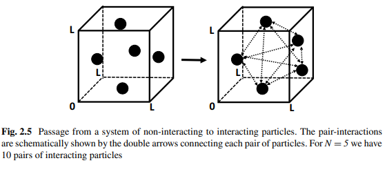
This change in Helmholtz energy corresponds to the process of “turning-on” the interaction among all the particles at constant $(T, V, N)$, Fig. 2.5.
The corresponding change in the entropy is:
$$
\begin{aligned}
\Delta S & =-\frac{\partial \Delta A}{\partial T}=\ln \frac{Z_N}{V^N}+T \frac{1}{Z_N} \frac{\partial Z_N}{\partial T} \
& =\ln Z_N-N \ln \mathrm{V}+\frac{1}{T} \int d R^N P\left(R^N\right) U_N\left(R^N\right)
\end{aligned}
$$
We now substitute $U_N\left(R^N\right)$ from (2.36) into (2.35) to obtain the expression for the change in entropy corresponding to “turning on” the interactions:
$$
\Delta S=-N \ln V-\int P\left(R^N\right) \ln P\left(R^N\right) d R^N
$$

信息论代写
数学代写|信息论代写information theory代考|The Forth Step: The SMI of Locations and Momenta
of N Independent Particles in a Box of Volume V.
Adding a Correction Due to Indistinguishability
of the Particles
最后一步是从盒子里的单个粒子,到体积$V$盒子里的$N$独立粒子,如图2.4所示。
我们说我们知道粒子的微观状态,当我们知道位置$(x, y, z)$,和盒子里一个粒子的动量$\left(p_x, p_y, p_z\right)$。对于盒子中含有$N$独立粒子的系统,我们可以将系统的SMI写成$N$乘以一个粒子的SMI,即:
$$
\mathrm{SMI}(N \text { independent particles })=N \times \mathrm{SMI} \text { (one particle) }
$$
这是$N$独立粒子的SMI。实际上,所有粒子的微观状态之间可能存在关联。我们将在这里提到由于粒子不可区分而产生的相关性,以及由于所有粒子之间的分子间相互作用而产生的相关性。我们将分别讨论这两种相关性的来源。回想一下,单个粒子的微观状态包括该粒子的位置和动量。让我们关注一个粒子在体积为$V$的盒子中的位置。我们将位置SMI写成:
$$
H_{\max }(\text { location })=\log V
$$
对于$N$独立粒子,我们将位置SMI写成:
$$
H_{\max } \text { (locations of N particles) }=\sum_{i=1}^N H_{\max }(\text { one particle })
$$
因为在现实中,粒子是不可区分的,我们必须修正式(2.22)。我们将粒子间关联所对应的互信息定义为:
$$
I(1 ; 2 ; \ldots ; N)=\ln N !
$$
因此,代替(2.22),对于$N$不可区分粒子的SMI,将写成:
$$
H(\text { Nparticles })=\sum_{i=1}^N H(\text { oneparticle })-\ln N !
$$
介绍$\ln N$的详细理由!由于粒子的不可分辨性,作为一种校正在Ben-Naim的5.2节中讨论[1]。这里我们将$N$不可区分(但不相互作用)粒子的SMI的最终结果写为:
$$
H(N \text { indistinguishable particles })=N \log V\left(\frac{2 \pi m e k_B T}{h^2}\right)^{3 / 2}-\log N !
$$
数学代写|信息论代写information theory代考|The Entropy of a System of Interacting Particles. Correlations Due to Intermolecular Interactions
在本节中,我们推导出相互作用粒子系统的SMI(或熵)与相应的互信息(MI)之间的最一般关系。在本章的后面,我们将把这个一般结果应用于一些具体的情况。这个结果的含义对于用SMI来解释熵的概念是非常重要的。换句话说,熵的“信息解释”被有效地扩展到所有处于平衡状态的相互作用粒子系统。
我们从经典统计力学的一些基本概念开始[7]。以变量$T, V, N$为特征的系统的经典正则配分函数(PF)为:
$$
Q(T, V, N)=\frac{Z_N}{N ! \Lambda^{3 N}}
$$
其中$\Lambda^3$称为动量配分函数(或德布罗意波长),$Z_N$是系统的构型PF”
$$
Z_N=\int \cdots \int d R^N \exp \left[-\beta U_N\left(R^N\right)\right]
$$
这里,$U_N\left(R^N\right)$是构型$R^N=R_1, \cdots, R_N$中$N$粒子之间的总相互作用能。统计热力学提供了在特定配置$R^N=R_1, \cdots, R_N$下找到粒子的概率密度,即:
$$
P\left(R^N\right)=\frac{\exp \left[-\beta U_N\left(R^N\right)\right]}{Z_N}
$$
其中$\beta=\left(k_B T\right)^{-1}$和$T$是绝对温度。下面我们选择$k_B=1$。这将促进熵变与SMI变化之间的联系。当不存在分子间相互作用(理想气体)时,构型$\mathrm{PF}$为$Z_N=V^N$,对应的配分函数化简为:
$$
Q^{i g}(T, V, N)=\frac{V^N}{N ! \Lambda^{3 N}}
$$
接下来我们将相互作用引起的亥姆霍兹能量$(A)$的变化定义为:
$$
\Delta A=A-A^{i g}=-T \ln \frac{Q(T, V, N)}{Q^{i g}(T, V, N)}=-T \ln \frac{Z_N}{V^N}
$$
亥姆霍兹能量的这种变化对应于在恒定$(T, V, N)$下“开启”所有粒子之间相互作用的过程,如图2.5所示。
对应的熵变为:
$$
\begin{aligned}
\Delta S & =-\frac{\partial \Delta A}{\partial T}=\ln \frac{Z_N}{V^N}+T \frac{1}{Z_N} \frac{\partial Z_N}{\partial T} \
& =\ln Z_N-N \ln \mathrm{V}+\frac{1}{T} \int d R^N P\left(R^N\right) U_N\left(R^N\right)
\end{aligned}
$$
现在我们将(2.36)中的$U_N\left(R^N\right)$代入(2.35),得到“开启”相互作用对应的熵变化表达式:
$$
\Delta S=-N \ln V-\int P\left(R^N\right) \ln P\left(R^N\right) d R^N
$$

统计代写请认准statistics-lab™. statistics-lab™为您的留学生涯保驾护航。
金融工程代写
金融工程是使用数学技术来解决金融问题。金融工程使用计算机科学、统计学、经济学和应用数学领域的工具和知识来解决当前的金融问题,以及设计新的和创新的金融产品。
非参数统计代写
非参数统计指的是一种统计方法,其中不假设数据来自于由少数参数决定的规定模型;这种模型的例子包括正态分布模型和线性回归模型。
广义线性模型代考
广义线性模型(GLM)归属统计学领域,是一种应用灵活的线性回归模型。该模型允许因变量的偏差分布有除了正态分布之外的其它分布。
术语 广义线性模型(GLM)通常是指给定连续和/或分类预测因素的连续响应变量的常规线性回归模型。它包括多元线性回归,以及方差分析和方差分析(仅含固定效应)。
有限元方法代写
有限元方法(FEM)是一种流行的方法,用于数值解决工程和数学建模中出现的微分方程。典型的问题领域包括结构分析、传热、流体流动、质量运输和电磁势等传统领域。
有限元是一种通用的数值方法,用于解决两个或三个空间变量的偏微分方程(即一些边界值问题)。为了解决一个问题,有限元将一个大系统细分为更小、更简单的部分,称为有限元。这是通过在空间维度上的特定空间离散化来实现的,它是通过构建对象的网格来实现的:用于求解的数值域,它有有限数量的点。边界值问题的有限元方法表述最终导致一个代数方程组。该方法在域上对未知函数进行逼近。[1] 然后将模拟这些有限元的简单方程组合成一个更大的方程系统,以模拟整个问题。然后,有限元通过变化微积分使相关的误差函数最小化来逼近一个解决方案。
tatistics-lab作为专业的留学生服务机构,多年来已为美国、英国、加拿大、澳洲等留学热门地的学生提供专业的学术服务,包括但不限于Essay代写,Assignment代写,Dissertation代写,Report代写,小组作业代写,Proposal代写,Paper代写,Presentation代写,计算机作业代写,论文修改和润色,网课代做,exam代考等等。写作范围涵盖高中,本科,研究生等海外留学全阶段,辐射金融,经济学,会计学,审计学,管理学等全球99%专业科目。写作团队既有专业英语母语作者,也有海外名校硕博留学生,每位写作老师都拥有过硬的语言能力,专业的学科背景和学术写作经验。我们承诺100%原创,100%专业,100%准时,100%满意。
随机分析代写
随机微积分是数学的一个分支,对随机过程进行操作。它允许为随机过程的积分定义一个关于随机过程的一致的积分理论。这个领域是由日本数学家伊藤清在第二次世界大战期间创建并开始的。
时间序列分析代写
随机过程,是依赖于参数的一组随机变量的全体,参数通常是时间。 随机变量是随机现象的数量表现,其时间序列是一组按照时间发生先后顺序进行排列的数据点序列。通常一组时间序列的时间间隔为一恒定值(如1秒,5分钟,12小时,7天,1年),因此时间序列可以作为离散时间数据进行分析处理。研究时间序列数据的意义在于现实中,往往需要研究某个事物其随时间发展变化的规律。这就需要通过研究该事物过去发展的历史记录,以得到其自身发展的规律。
回归分析代写
多元回归分析渐进(Multiple Regression Analysis Asymptotics)属于计量经济学领域,主要是一种数学上的统计分析方法,可以分析复杂情况下各影响因素的数学关系,在自然科学、社会和经济学等多个领域内应用广泛。
MATLAB代写
MATLAB 是一种用于技术计算的高性能语言。它将计算、可视化和编程集成在一个易于使用的环境中,其中问题和解决方案以熟悉的数学符号表示。典型用途包括:数学和计算算法开发建模、仿真和原型制作数据分析、探索和可视化科学和工程图形应用程序开发,包括图形用户界面构建MATLAB 是一个交互式系统,其基本数据元素是一个不需要维度的数组。这使您可以解决许多技术计算问题,尤其是那些具有矩阵和向量公式的问题,而只需用 C 或 Fortran 等标量非交互式语言编写程序所需的时间的一小部分。MATLAB 名称代表矩阵实验室。MATLAB 最初的编写目的是提供对由 LINPACK 和 EISPACK 项目开发的矩阵软件的轻松访问,这两个项目共同代表了矩阵计算软件的最新技术。MATLAB 经过多年的发展,得到了许多用户的投入。在大学环境中,它是数学、工程和科学入门和高级课程的标准教学工具。在工业领域,MATLAB 是高效研究、开发和分析的首选工具。MATLAB 具有一系列称为工具箱的特定于应用程序的解决方案。对于大多数 MATLAB 用户来说非常重要,工具箱允许您学习和应用专业技术。工具箱是 MATLAB 函数(M 文件)的综合集合,可扩展 MATLAB 环境以解决特定类别的问题。可用工具箱的领域包括信号处理、控制系统、神经网络、模糊逻辑、小波、仿真等。