如果你也在 怎样代写线性规划Linear Programming这个学科遇到相关的难题,请随时右上角联系我们的24/7代写客服。
线性规划,数学建模技术,其中一个线性函数在受到各种约束时被最大化或最小化。这种技术对于指导商业规划、工业工程中的定量决策非常有用,在较小的程度上也适用于社会和物理科学。
statistics-lab™ 为您的留学生涯保驾护航 在代写线性规划Linear Programming方面已经树立了自己的口碑, 保证靠谱, 高质且原创的统计Statistics代写服务。我们的专家在代写线性规划Linear Programming代写方面经验极为丰富,各种代写线性规划Linear Programming相关的作业也就用不着说。
我们提供的线性规划Linear Programming及其相关学科的代写,服务范围广, 其中包括但不限于:
- Statistical Inference 统计推断
- Statistical Computing 统计计算
- Advanced Probability Theory 高等概率论
- Advanced Mathematical Statistics 高等数理统计学
- (Generalized) Linear Models 广义线性模型
- Statistical Machine Learning 统计机器学习
- Longitudinal Data Analysis 纵向数据分析
- Foundations of Data Science 数据科学基础
数学代写|线性规划作业代写Linear Programming代考|Conic Combination Interpretations
This basis transformation, as illustrated in Sect. 3.3, can be interpreted as in requirements space, the space where the columns of $\mathbf{A}$ and $\mathbf{b}$ are represented. The fundamental relation is
$$
\mathbf{a}_1 x_1+\mathbf{a}_2 x_2+\cdots+\mathbf{a}_n x_n=\mathbf{b} .
$$
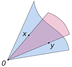
An example for $m=2, n=4$ is shown in Fig. $4.1$.
A feasible solution defines a representation of $\mathbf{b}$ as a conic combination of the $\mathbf{a}_i$ ‘s. A basic feasible solution will use only $m$ positive weights. In the figure a basic feasible solution can be constructed with positive weights on $\mathbf{a}_1$ and $\mathbf{a}_2$ because $\mathbf{b}$ lies between them. A basic feasible solution cannot be constructed with positive weights on $\mathbf{a}_1$ and $\mathbf{a}_4$. Suppose we start with $\mathbf{a}_1$ and $\mathbf{a}_2$ as the initial basis. Then an adjacent basis is found by bringing in some other vector. If $\mathbf{a}_3$ is brought in, then clearly $\mathbf{a}_2$ must go out. On the other hand, if $\mathbf{a}_4$ is brought in, $\mathbf{a}_1$ must go out. In summary, we have deduced that, given a basic feasible solution and an arbitrary vector $\mathbf{a}_e$, there is either a new basic feasible solution having $\mathbf{a}_e$ in its basis and one of the original vectors removed, or the set of feasible solutions is unbounded.
Of course, another interpretation is in activity space, the space where $\mathbf{x}$ is represented. This is perhaps the most natural space to consider, especially with only inequality constraints. Here the feasible region is shown directly as a convex set, and basic feasible solutions are extreme points. Adjacent extreme points are points that lie on a common edge.
Example 1 (Basis Change Illustration) Consider the equality constraints of Example 1 of Sect. 3.3:
$$
\begin{array}{r}
3 x_1+x_2-2 x_3+x_4=2 \
x_1+3 x_2-x_4=2 .
\end{array}
$$
Suppose we start with $\mathbf{a}_1$ and $\mathbf{a}_2$ as the initial basis and select $\mathbf{a}_3$ as the incoming column. Then
$$
\mathbf{B}=\left(\begin{array}{ll}
3 & 1 \
1 & 3
\end{array}\right), \mathbf{B}^{-1}=\left(\begin{array}{cc}
3 / 8 & 1 / 8 \
-1 / 8 & 3 / 8
\end{array}\right), \overline{\mathbf{a}}_0=\mathbf{B}^{-1} \mathbf{b}=\left(\begin{array}{l}
1 / 2 \
1 / 2
\end{array}\right), \overline{\mathbf{a}}_3=\mathbf{B}^{-1} \mathbf{a}_3=\left(\begin{array}{c}
-3 / 4 \
1 / 4
\end{array}\right) .
$$
From (4.5), $\varepsilon=2$ and $\mathbf{a}_2$ is the outgoing column so that the new basis is formed by $\mathbf{a}_1$ and $\mathbf{a}_3$.
Now suppose we start with $\mathbf{a}_1$ and $\mathbf{a}_3$ as the initial basis and select $\mathbf{a}_4$ as the incoming column. Then
$$
\mathbf{B}=\left(\begin{array}{cc}
3 & 1 \
-2 & 0
\end{array}\right), \mathbf{B}^{-1}=\left(\begin{array}{cc}
0 & 1 \
-1 / 2 & 3 / 2
\end{array}\right), \overline{\mathbf{a}}_0=\mathbf{B}^{-1} \mathbf{b}=\left(\begin{array}{l}
2 \
2
\end{array}\right), \overline{\mathbf{a}}_4=\mathbf{B}^{-1} \mathbf{a}_4=\left(\begin{array}{l}
-1 \
-2
\end{array}\right) .
$$
Since the entries of the incoming column $\overline{\mathbf{a}}_4$ are all negative, $\varepsilon$ in (4.5) can go to $\infty$, indicating that the feasible region is unbounded.
数学代写|线性规划作业代写Linear Programming代考|Finding an Initial Basic Feasible Solution
The simplex procedure needs to start from a basic feasible solution. A basic feasible solution is sometimes immediately available for linear programs. For example, in resource-allocation/production problems with constraints of the form
$$
\mathbf{A x} \leqslant \mathbf{b}, \quad \mathbf{x} \geqslant \mathbf{0}
$$
with $\mathbf{b} \geqslant \mathbf{0}$, a basic feasible solution to the corresponding standard form of the problem is provided by the slack variables. This provides a means for initiating the simplex procedure. The example in the last section was of this type. An initial basic feasible solution is not always apparent for other types of linear programs, however, and it is necessary to develop a means for determining one so that the simplex method can be initiated. Interestingly (and fortunately), an auxiliary linear program and corresponding application of the simplex method can be used to determine the required initial solution.
By elementary straightforward operations the constraints of a linear programming problem can always be expressed in the so-called Phase I form
$$
\mathbf{A x}=\mathbf{b}, \quad \mathbf{x} \geqslant \mathbf{0}
$$ with $\mathbf{b} \geqslant \mathbf{0}$. Generally, in order to find a solution to (4.13) consider the artificial minimization problem (commonly called the Phase One linear program).
$$
\begin{array}{ll}
\operatorname{minimize} & \sum_{i=1}^m u_j \
\text { subject to } & \mathbf{A x}+\mathbf{u}=\mathbf{b} \
& \mathbf{x} \geqslant \mathbf{0}, \mathbf{u} \geqslant \mathbf{0},
\end{array}
$$
where $\mathbf{u}=\left(u_1, u_2, \ldots, u_m\right)$ is a vector of artificial variables. If there is a feasible solution to (4.13), then it is clear that (4.14) has a minimum value of zero with $\mathbf{u}=\mathbf{0}$. If (4.13) has no feasible solution, then the minimum value of (4.14) is greater than zero.
Now (4.14) is itself a linear program in the variables $\mathbf{x}, \mathbf{u}$, and the system is already in canonical form with basic feasible solution $\mathbf{u}=\mathbf{b}$. If (4.14) is solved using the simplex technique, a basic feasible solution is obtained at each step. If the minimum value of (4.14) is zero, then the final basic solution will have all $u_j=0$, and hence barring degeneracy, the final solution will have no $u_j$ variables basic. If in the final solution some $u_j$ are both zero and basic, indicating a degenerate solution, these basic variables can be exchanged for nonbasic $x_j$ variables (again at zero level) to yield a basic feasible solution involving $x$ variables only. Then one can proceed to minimize the original objective called Phase II.
线性规划代写
数学代写|线性规划作业代写Linear Programming代考|Conic Combination Interpretations
这种基础转变,如第 1 节所示。3.3、可以理解为在requirements space中,列所在的空间 $\mathbf{A}$ 和 $\mathbf{b}$ 有代 表。基本关系是
$$
\mathbf{a}_1 x_1+\mathbf{a}_2 x_2+\cdots+\mathbf{a}_n x_n=\mathbf{b} .
$$
一个例子 $m=2, n=4$ 如图所示 $4.1$.
一个可行的解决方案定义了一个表示 $\mathbf{b}$ 作为圆雉曲线的组合 $\mathbf{a}_i$ 的。一个基本可行的解决方案将只使用 $m$ 正 权重。在图中,可以构造一个基本可行的解决方案,其中权重为正 $\mathbf{a}_1$ 和 $\mathbf{a}_2$ 因为 $\mathbf{b}$ 位于他们之间。不能用 正权重构造基本可行解 $\mathbf{a}_1$ 和 $\mathbf{a}_4$. 假设我们开始 $\mathbf{a}_1$ 和 $\mathbf{a}_2$ 作为初始依据。然后通过引入一些其他向量来找到 相邻的基础。如果 $\mathbf{a}_3$ 被带进来,那么很明显 $\mathbf{a}_2$ 必须出去。另一方面,如果 $\mathbf{a}_4$ 被带进来, $\mathbf{a}_1$ 必须出去。总 之,我们推导出,给定一个基本可行解和一个任意向量 $\mathbf{a}_e$ ,要么有一个新的基本可行解 $\mathbf{a}_e$ 在它的基础上, 删除了一个原始向量,或者可行解集是无界的。
当然,另一种解释是在活动空间,空间 $\mathbf{x}$ 被代表。这可能是最自然要考虑的空间,尤其是在只有不平等约 束的情况下。这里可行域直接表示为凸集,基本可行解为极值点。相邻极值点是位于公共边上的点。
示例 1 (基础变化说明) 考虑第 1 节示例 1 的等式约束。 $3.3$ :
$$
3 x_1+x_2-2 x_3+x_4=2 x_1+3 x_2-x_4=2 .
$$
假设我们开始 $\mathbf{a}_1$ 和 $\mathbf{a}_2$ 作为初始依据并选择 $\mathbf{a}_3$ 作为传入列。然后
从 (4.5), $\varepsilon=2$ 和 $\mathbf{a}_2$ 是输出列,因此新基础由 $\mathbf{a}_1$ 和 $\mathbf{a}_3$.
现在假设我们开始 $\mathbf{a}_1$ 和 $\mathbf{a}_3$ 作为初始依据并选择 $\mathbf{a}_4$ 作为传入列。然后
由于传入列的条目 $\overline{\mathbf{a}}_4$ 都是负面的, $\varepsilon$ 在 (4.5) 中可以转到 $\infty$ ,表明可行域是无界的。
数学代写|线性规划作业代写Linear Programming代考|Finding an Initial Basic Feasible Solution
单纯形法需要从一个基本可行解开始。对于线性规划,有时可以立即获得基本可行解。例如,在具有形式 约束的资源分配/生产问题中
$$
\mathbf{A} \mathbf{x} \leqslant \mathbf{b}, \quad \mathbf{x} \geqslant \mathbf{0}
$$
和 $\mathbf{b} \geqslant \mathbf{0}$ ,松他变量提供了问题相应标准形式的基本可行解。这提供了一种启动单纯形程序的方法。上 一节中的示例就是这种类型。然而,对于其他类型的线性规划,初始基本可行解并不总是显而易见的,因 此有必要开发一种方法来确定一个,以便可以启动单纯形法。有趣的是(幸运的是)辅助线性程序和单纯 形法的相应应用可用于确定所需的初始解。
通过基本的直接操作,线性规划问题的约束总是可以用所谓的阶段 I 形式表示
$$
\mathbf{A} \mathbf{x}=\mathbf{b}, \quad \mathbf{x} \geqslant \mathbf{0}
$$
和 $\mathbf{b} \geqslant \mathbf{0}$. 通常,为了找到 (4.13) 的解,考虑人工最小化问题(通常称为第一阶段线性规划) 。
$$
\operatorname{minimize} \quad \sum_{i=1}^m u_j \text { subject to } \quad \mathbf{A x}+\mathbf{u}=\mathbf{b} \quad \mathbf{x} \geqslant \mathbf{0}, \mathbf{u} \geqslant \mathbf{0}
$$
在哪里 $\mathbf{u}=\left(u_1, u_2, \ldots, u_m\right)$ 是人工变量的向量。如果 (4.13) 有可行解,则很明显 (4.14) 的最小值为零 $\mathbf{u}=\mathbf{0}$. 如果 (4.13) 没有可行解,则 (4.14) 的最小值大于零。
现在 (4.14) 本身是变量中的线性程序 $\mathbf{x}, \mathbf{u}$, 并且系统已经是具有基本可行解的规范形式 $\mathbf{u}=\mathbf{b}$. 如果使用 单纯形法求解 (4.14),则在每一步都会得到一个基本可行解。如果 (4.14) 的最小值为零,那么最终的基 本解将有所有 $u_j=0$ ,因此除非退化,最终的解决方案将没有 $u_j$ 变量基本。如果在最终解决方案中一些 $u_j$ 既是零又是基数,表示退化解,这些基数变量可以换成非基数 $x_j$ 变量(再次为零水平)以产生一个基 本可行的解决方案,包括 $x$ 只有变量。然后可以继续最小化称为第二阶段的原始目标。

统计代写请认准statistics-lab™. statistics-lab™为您的留学生涯保驾护航。
金融工程代写
金融工程是使用数学技术来解决金融问题。金融工程使用计算机科学、统计学、经济学和应用数学领域的工具和知识来解决当前的金融问题,以及设计新的和创新的金融产品。
非参数统计代写
非参数统计指的是一种统计方法,其中不假设数据来自于由少数参数决定的规定模型;这种模型的例子包括正态分布模型和线性回归模型。
广义线性模型代考
广义线性模型(GLM)归属统计学领域,是一种应用灵活的线性回归模型。该模型允许因变量的偏差分布有除了正态分布之外的其它分布。
术语 广义线性模型(GLM)通常是指给定连续和/或分类预测因素的连续响应变量的常规线性回归模型。它包括多元线性回归,以及方差分析和方差分析(仅含固定效应)。
有限元方法代写
有限元方法(FEM)是一种流行的方法,用于数值解决工程和数学建模中出现的微分方程。典型的问题领域包括结构分析、传热、流体流动、质量运输和电磁势等传统领域。
有限元是一种通用的数值方法,用于解决两个或三个空间变量的偏微分方程(即一些边界值问题)。为了解决一个问题,有限元将一个大系统细分为更小、更简单的部分,称为有限元。这是通过在空间维度上的特定空间离散化来实现的,它是通过构建对象的网格来实现的:用于求解的数值域,它有有限数量的点。边界值问题的有限元方法表述最终导致一个代数方程组。该方法在域上对未知函数进行逼近。[1] 然后将模拟这些有限元的简单方程组合成一个更大的方程系统,以模拟整个问题。然后,有限元通过变化微积分使相关的误差函数最小化来逼近一个解决方案。
tatistics-lab作为专业的留学生服务机构,多年来已为美国、英国、加拿大、澳洲等留学热门地的学生提供专业的学术服务,包括但不限于Essay代写,Assignment代写,Dissertation代写,Report代写,小组作业代写,Proposal代写,Paper代写,Presentation代写,计算机作业代写,论文修改和润色,网课代做,exam代考等等。写作范围涵盖高中,本科,研究生等海外留学全阶段,辐射金融,经济学,会计学,审计学,管理学等全球99%专业科目。写作团队既有专业英语母语作者,也有海外名校硕博留学生,每位写作老师都拥有过硬的语言能力,专业的学科背景和学术写作经验。我们承诺100%原创,100%专业,100%准时,100%满意。
随机分析代写
随机微积分是数学的一个分支,对随机过程进行操作。它允许为随机过程的积分定义一个关于随机过程的一致的积分理论。这个领域是由日本数学家伊藤清在第二次世界大战期间创建并开始的。
时间序列分析代写
随机过程,是依赖于参数的一组随机变量的全体,参数通常是时间。 随机变量是随机现象的数量表现,其时间序列是一组按照时间发生先后顺序进行排列的数据点序列。通常一组时间序列的时间间隔为一恒定值(如1秒,5分钟,12小时,7天,1年),因此时间序列可以作为离散时间数据进行分析处理。研究时间序列数据的意义在于现实中,往往需要研究某个事物其随时间发展变化的规律。这就需要通过研究该事物过去发展的历史记录,以得到其自身发展的规律。
回归分析代写
多元回归分析渐进(Multiple Regression Analysis Asymptotics)属于计量经济学领域,主要是一种数学上的统计分析方法,可以分析复杂情况下各影响因素的数学关系,在自然科学、社会和经济学等多个领域内应用广泛。
MATLAB代写
MATLAB 是一种用于技术计算的高性能语言。它将计算、可视化和编程集成在一个易于使用的环境中,其中问题和解决方案以熟悉的数学符号表示。典型用途包括:数学和计算算法开发建模、仿真和原型制作数据分析、探索和可视化科学和工程图形应用程序开发,包括图形用户界面构建MATLAB 是一个交互式系统,其基本数据元素是一个不需要维度的数组。这使您可以解决许多技术计算问题,尤其是那些具有矩阵和向量公式的问题,而只需用 C 或 Fortran 等标量非交互式语言编写程序所需的时间的一小部分。MATLAB 名称代表矩阵实验室。MATLAB 最初的编写目的是提供对由 LINPACK 和 EISPACK 项目开发的矩阵软件的轻松访问,这两个项目共同代表了矩阵计算软件的最新技术。MATLAB 经过多年的发展,得到了许多用户的投入。在大学环境中,它是数学、工程和科学入门和高级课程的标准教学工具。在工业领域,MATLAB 是高效研究、开发和分析的首选工具。MATLAB 具有一系列称为工具箱的特定于应用程序的解决方案。对于大多数 MATLAB 用户来说非常重要,工具箱允许您学习和应用专业技术。工具箱是 MATLAB 函数(M 文件)的综合集合,可扩展 MATLAB 环境以解决特定类别的问题。可用工具箱的领域包括信号处理、控制系统、神经网络、模糊逻辑、小波、仿真等。