如果你也在 怎样代写线性回归分析linear regression analysis这个学科遇到相关的难题,请随时右上角联系我们的24/7代写客服。
回归分析是一种强大的统计方法,允许你检查两个或多个感兴趣的变量之间的关系。虽然有许多类型的回归分析,但它们的核心都是考察一个或多个自变量对因变量的影响。
statistics-lab™ 为您的留学生涯保驾护航 在代写线性回归分析linear regression analysis方面已经树立了自己的口碑, 保证靠谱, 高质且原创的统计Statistics代写服务。我们的专家在代写线性回归分析linear regression analysis代写方面经验极为丰富,各种代写线性回归分析linear regression analysis相关的作业也就用不着说。
我们提供的线性回归分析linear regression analysis及其相关学科的代写,服务范围广, 其中包括但不限于:
- Statistical Inference 统计推断
- Statistical Computing 统计计算
- Advanced Probability Theory 高等楖率论
- Advanced Mathematical Statistics 高等数理统计学
- (Generalized) Linear Models 广义线性模型
- Statistical Machine Learning 统计机器学习
- Longitudinal Data Analysis 纵向数据分析
- Foundations of Data Science 数据科学基础
统计代写|线性回归分析代写linear regression analysis代考|Plots for the Multivariate Linear Regression Model
This section suggests using residual plots, response plots, and the DD plot to examine the multivariate linear model. The residual plots are often used to check for lack of fit of the multivariate linear model. The response plots are used to check linearity and to detect influential cases and outliers. The response and residual plots are used exactly as in the $m=1$ case corresponding to multiple linear regression and experimental design models. See earlier chapters of this book, Olive et al. (2015), Olive and Hawkins (2005), and Cook and Weisberg (1999a, p. 432; 1999b).
Notation. Plots will be used to simplify the regression analysis, and in this text a plot of $W$ versus $Z$ uses $W$ on the horizontal axis and $Z$ on the vertical axis.
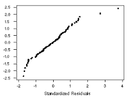
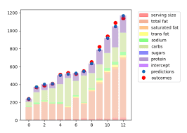
Definition 12.5. A response plot for the $j$ th response variable is a plot of the fitted values $\widehat{Y}{i j}$ versus the response $Y{i j}$. The identity line with slope one and zero intercept is added to the plot as a visual aid. A residual plot corresponding to the $j$ th response variable is a plot of $\hat{Y}{i j}$ versus $r{i j}$.
Remark 12.1. Make the $m$ response and residual plots for any multivariate linear regression. In a response plot, the vertical deviations from the identity line are the residuals $r_{i j}=Y_{i j}-\hat{Y}_{i j}$. Suppose the model is good, the $j$ th error distribution is unimodal and not highly skewed for $j=1, \ldots, m$, and $n \geq 10 p$. Then the plotted points should cluster about the identity line in each of the $m$ response plots. If outliers are present or if the plot is not linear, then the current model or data need to be transformed or corrected. If the model is good, then each of the $m$ residual plots should be ellipsoidal with no trend and should be centered about the $r=0$ line. There should not be any pattern in the residual plot: as a narrow vertical strip is moved from left to right, the behavior of the residuals within the strip should show little change. Outliers and patterns such as curvature or a fan shaped plot are bad.
统计代写|线性回归分析代写linear regression analysis代考|Asymptotically Optimal Prediction Regions
In this section, we will consider a more general multivariate regression model, and then consider the multivariate linear model as a special case. Given $n$ cases of training or past data $\left(\boldsymbol{x}_1, \boldsymbol{y}_1\right), \ldots,\left(\boldsymbol{x}_n, \boldsymbol{y}_n\right)$ and a vector of predictors $\boldsymbol{x}_f$, suppose it is desired to predict a future test vector $\boldsymbol{y}_f$.
Definition 12.8. A large sample $100(1-\delta) \%$ prediction region is a set $\mathcal{A}_n$ such that $P\left(\boldsymbol{y}_f \in \mathcal{A}_n\right) \rightarrow 1-\delta$ as $n \rightarrow \infty$, and is asymptotically optimal if the volume of the region converges in probability to the volume of the population minimum volume covering region.
The classical large sample $100(1-\delta) \%$ prediction region for a future value $\boldsymbol{x}f$ given iid data $\boldsymbol{x}_1, \ldots, \boldsymbol{x}_n$ is $\left{\boldsymbol{x}: D{\boldsymbol{x}}^2(\overline{\boldsymbol{x}}, \boldsymbol{S}) \leq \chi_{p, 1-\delta}^2\right}$, while for multivariate linear regression, the classical large sample $100(1-\delta) \%$ prediction region for a future value $\boldsymbol{y}f$ given $\boldsymbol{x}_f$ and past data $\left(\boldsymbol{x}_1, \boldsymbol{y}_i\right), \ldots,\left(\boldsymbol{x}_n, \boldsymbol{y}_n\right)$ is $\left{\boldsymbol{y}: D{\boldsymbol{y}}^2\left(\hat{\boldsymbol{y}}f, \hat{\boldsymbol{\Sigma}}{\boldsymbol{\epsilon}}\right) \leq \chi_{m, 1-\delta}^2\right}$. See Johnson and Wichern (1988, pp. 134, 151, $312)$. By equation $(10.10)$, these regions may work for multivariate normal $\boldsymbol{x}i$ or $\boldsymbol{\epsilon}_i$, but otherwise tend to have undercoverage. Olive (2013a) replaced $\chi{p, 1-\delta}^2$ by the order statistic $D_{\left(U_n\right)}^2$ where $U_n$ decreases to $\lceil n(1-\delta)\rceil$. This section will use a similar technique from Olive (2016b) to develop possibly the first practical large sample prediction region for the multivariate linear model with unknown error distribution. The following technical theorem will be needed to prove Theorem 12.4.
Theorem 12.3. Let $a>0$ and assume that $\left(\hat{\boldsymbol{\mu}}n, \hat{\boldsymbol{\Sigma}}_n\right)$ is a consistent estimator of $(\boldsymbol{\mu}, a \boldsymbol{\Sigma})$. a) $D{\boldsymbol{x}}^2\left(\hat{\boldsymbol{\mu}}n, \hat{\boldsymbol{\Sigma}}_n\right)-\frac{1}{a} D{\boldsymbol{x}}^2(\boldsymbol{\mu}, \boldsymbol{\Sigma})=o_P(1)$.
b) Let $0<\delta \leq 0.5$. If $\left(\hat{\boldsymbol{\mu}}n, \hat{\boldsymbol{\Sigma}}_n\right)-(\boldsymbol{\mu}, a \boldsymbol{\Sigma})=O_p\left(n^{-\delta}\right)$ and $a \hat{\boldsymbol{\Sigma}}_n^{-1}-\boldsymbol{\Sigma}^{-1}=$ $O_P\left(n^{-\delta}\right)$, then $$ D{\boldsymbol{x}}^2\left(\hat{\boldsymbol{\mu}}n, \hat{\boldsymbol{\Sigma}}_n\right)-\frac{1}{a} D{\boldsymbol{x}}^2(\boldsymbol{\mu}, \boldsymbol{\Sigma})=O_P\left(n^{-\delta}\right)
$$
线性回归代写
统计代写|线性回归分析代写linear regression analysis代考|Plots for the Multivariate Linear Regression Model
本节建议使用残差图、响应图和 DD 图来检查多元线性模型。残差图通常用于检查多元线性模型的拟合 不足。响应图用于检查线性并检测有影响的个案和离群值。响应图和残差图的使用与 $m=1$ 对应于多元 线性回归和实验设计模型的案例。请参阅本书的前几章,Olive 等人。(2015)、Olive 和 Hawkins (2005),以及 Cook 和 Weisberg (1999a, p. 432; 1999b)。
符号。绘图将用于简化回归分析,在本文中的绘图 $W$ 相对 $Z$ 使用 $W$ 在水平轴上和 $Z$ 在垂直轴上。
定义 12.5。的响应图 $j$ 第一个响应变量是拟合值图 $\widehat{Y} i j$ 与响应 $Y i j$. 带有斜率 1 和零截距的标识线作为视 觉辅助添加到图中。残差图对应于 $j$ 第一个响应变量是 $\hat{Y} i j$ 相对 $r i j$.
备注 12.1。让 $m$ 任何多元线性回归的响应和残差图。在响应图中,与标识线的垂直偏差是残差 $r_{i j}=Y_{i j}-\hat{Y}_{i j}$. 假设模型很好,则 $j$ th 错误分布是单峰的并且不是高度偏斜的 $j=1, \ldots, m$ ,和 $n \geq 10 p$. 然后绘制的点应该聚集在每个 $m$ 响应图。如果存在异常值或绘图不是线性的,则需要转换或校 正当前模型或数据。如果模型很好,那么每个 $m$ 残差图应该是没有趋势的椭圆形,并且应该以 $r=0$ 线。残差图中不应该有任何模式:当一个宱的垂直条带从左向右移动时,条带内残差的行为应该显示出 很小的变化。曲率或扇形图等异常值和模式是不好的。
统计代写|线性回归分析代写linear regression analysis代考|Asymptotically Optimal Prediction Regions
在本节中,我们将考虑更一般的多元回归模型,然后将多元线性模型视为特例。鉴于 $n$ 训练案例或过去的 数据 $\left(\boldsymbol{x}1, \boldsymbol{y}_1\right), \ldots,\left(\boldsymbol{x}_n, \boldsymbol{y}_n\right)$ 和一个预测向量 $\boldsymbol{x}_f$ ,假设需要预测末来的测试向量 $\boldsymbol{y}_f$. 定义 12.8。大样本 $100(1-\delta) \%$ 预测区域是一个集合 $\mathcal{A}_n$ 这样 $P\left(\boldsymbol{y}_f \in \mathcal{A}_n\right) \rightarrow 1-\delta$ 作为 $n \rightarrow \infty$ , 并且如果该区域的体积在概率上收敛于人口最小体积覆盖区域的体积,则它是渐近最优的。 经典大样本 $100(1-\delta) \%$ 末来值的预测区域 $\boldsymbol{x}$ 给定的 iid 数据 $\boldsymbol{x}_1, \ldots, \boldsymbol{x}_n$ 是 ,而对于多元线性回归,经典的大样本 $100(1-\delta) \%$ 末来值的预测区域 $\boldsymbol{y} f$ 给予 $\boldsymbol{x}_f$ 和过去的数据 $\left(\boldsymbol{x}_1, \boldsymbol{y}_i\right), \ldots,\left(\boldsymbol{x}_n, \boldsymbol{y}_n\right)$ 是 . 参见 Johnson 和 Wichern (1988 年,第 134、151 页,312). 通过等式 (10.10),这些区域可能适用 于多元正态 $\boldsymbol{x} i$ 或者 $\boldsymbol{\epsilon}_i$ ,但在其他方面往往有隐蔽性。橄榄 (2013a) 替换 $\chi p, 1-\delta^2$ 按顺序统计 $D{\left(U_n\right)}^2$ 在哪 里 $U_n$ 减少到 $\lceil n(1-\delta)\rceil$. 本节将使用 Olive (2016b) 中的类似技术,为具有末知误差分布的多元线性模 型开发可能是第一个实用的大样本预测区域。需要下面的技术定理来证明定理 12.4。
定理 12.3。让 $a>0$ 并假设 $\left(\hat{\boldsymbol{\mu}} n, \hat{\boldsymbol{\Sigma}}_n\right)$ 是一致的估计量 $(\boldsymbol{\mu}, a \boldsymbol{\Sigma})$. A)
$$
D \boldsymbol{x}^2\left(\hat{\boldsymbol{\mu}} n, \hat{\boldsymbol{\Sigma}}_n\right)-\frac{1}{a} D \boldsymbol{x}^2(\boldsymbol{\mu}, \boldsymbol{\Sigma})=o_P(1)
$$
b) 让 $0<\delta \leq 0.5$. 如果 $\left(\hat{\boldsymbol{\mu}} n, \hat{\mathbf{\Sigma}}_n\right)-(\boldsymbol{\mu}, a \boldsymbol{\Sigma})=O_p\left(n^{-\delta}\right)$ 和 $a \hat{\mathbf{\Sigma}}_n^{-1}-\boldsymbol{\Sigma}^{-1}=O_P\left(n^{-\delta}\right)$ ,然后
$$
D \boldsymbol{x}^2\left(\hat{\boldsymbol{\mu}} n, \hat{\boldsymbol{\Sigma}}_n\right)-\frac{1}{a} D \boldsymbol{x}^2(\boldsymbol{\mu}, \mathbf{\Sigma})=O_P\left(n^{-\delta}\right)
$$

统计代写请认准statistics-lab™. statistics-lab™为您的留学生涯保驾护航。
随机过程代考
在概率论概念中,随机过程是随机变量的集合。 若一随机系统的样本点是随机函数,则称此函数为样本函数,这一随机系统全部样本函数的集合是一个随机过程。 实际应用中,样本函数的一般定义在时间域或者空间域。 随机过程的实例如股票和汇率的波动、语音信号、视频信号、体温的变化,随机运动如布朗运动、随机徘徊等等。
贝叶斯方法代考
贝叶斯统计概念及数据分析表示使用概率陈述回答有关未知参数的研究问题以及统计范式。后验分布包括关于参数的先验分布,和基于观测数据提供关于参数的信息似然模型。根据选择的先验分布和似然模型,后验分布可以解析或近似,例如,马尔科夫链蒙特卡罗 (MCMC) 方法之一。贝叶斯统计概念及数据分析使用后验分布来形成模型参数的各种摘要,包括点估计,如后验平均值、中位数、百分位数和称为可信区间的区间估计。此外,所有关于模型参数的统计检验都可以表示为基于估计后验分布的概率报表。
广义线性模型代考
广义线性模型(GLM)归属统计学领域,是一种应用灵活的线性回归模型。该模型允许因变量的偏差分布有除了正态分布之外的其它分布。
statistics-lab作为专业的留学生服务机构,多年来已为美国、英国、加拿大、澳洲等留学热门地的学生提供专业的学术服务,包括但不限于Essay代写,Assignment代写,Dissertation代写,Report代写,小组作业代写,Proposal代写,Paper代写,Presentation代写,计算机作业代写,论文修改和润色,网课代做,exam代考等等。写作范围涵盖高中,本科,研究生等海外留学全阶段,辐射金融,经济学,会计学,审计学,管理学等全球99%专业科目。写作团队既有专业英语母语作者,也有海外名校硕博留学生,每位写作老师都拥有过硬的语言能力,专业的学科背景和学术写作经验。我们承诺100%原创,100%专业,100%准时,100%满意。
机器学习代写
随着AI的大潮到来,Machine Learning逐渐成为一个新的学习热点。同时与传统CS相比,Machine Learning在其他领域也有着广泛的应用,因此这门学科成为不仅折磨CS专业同学的“小恶魔”,也是折磨生物、化学、统计等其他学科留学生的“大魔王”。学习Machine learning的一大绊脚石在于使用语言众多,跨学科范围广,所以学习起来尤其困难。但是不管你在学习Machine Learning时遇到任何难题,StudyGate专业导师团队都能为你轻松解决。
多元统计分析代考
基础数据: $N$ 个样本, $P$ 个变量数的单样本,组成的横列的数据表
变量定性: 分类和顺序;变量定量:数值
数学公式的角度分为: 因变量与自变量
时间序列分析代写
随机过程,是依赖于参数的一组随机变量的全体,参数通常是时间。 随机变量是随机现象的数量表现,其时间序列是一组按照时间发生先后顺序进行排列的数据点序列。通常一组时间序列的时间间隔为一恒定值(如1秒,5分钟,12小时,7天,1年),因此时间序列可以作为离散时间数据进行分析处理。研究时间序列数据的意义在于现实中,往往需要研究某个事物其随时间发展变化的规律。这就需要通过研究该事物过去发展的历史记录,以得到其自身发展的规律。
回归分析代写
多元回归分析渐进(Multiple Regression Analysis Asymptotics)属于计量经济学领域,主要是一种数学上的统计分析方法,可以分析复杂情况下各影响因素的数学关系,在自然科学、社会和经济学等多个领域内应用广泛。
MATLAB代写
MATLAB 是一种用于技术计算的高性能语言。它将计算、可视化和编程集成在一个易于使用的环境中,其中问题和解决方案以熟悉的数学符号表示。典型用途包括:数学和计算算法开发建模、仿真和原型制作数据分析、探索和可视化科学和工程图形应用程序开发,包括图形用户界面构建MATLAB 是一个交互式系统,其基本数据元素是一个不需要维度的数组。这使您可以解决许多技术计算问题,尤其是那些具有矩阵和向量公式的问题,而只需用 C 或 Fortran 等标量非交互式语言编写程序所需的时间的一小部分。MATLAB 名称代表矩阵实验室。MATLAB 最初的编写目的是提供对由 LINPACK 和 EISPACK 项目开发的矩阵软件的轻松访问,这两个项目共同代表了矩阵计算软件的最新技术。MATLAB 经过多年的发展,得到了许多用户的投入。在大学环境中,它是数学、工程和科学入门和高级课程的标准教学工具。在工业领域,MATLAB 是高效研究、开发和分析的首选工具。MATLAB 具有一系列称为工具箱的特定于应用程序的解决方案。对于大多数 MATLAB 用户来说非常重要,工具箱允许您学习和应用专业技术。工具箱是 MATLAB 函数(M 文件)的综合集合,可扩展 MATLAB 环境以解决特定类别的问题。可用工具箱的领域包括信号处理、控制系统、神经网络、模糊逻辑、小波、仿真等。