如果你也在 怎样代写机器学习 machine learning这个学科遇到相关的难题,请随时右上角联系我们的24/7代写客服。
机器学习是一个致力于理解和建立 “学习 “方法的研究领域,也就是说,利用数据来提高某些任务的性能的方法。机器学习算法基于样本数据(称为训练数据)建立模型,以便在没有明确编程的情况下做出预测或决定。机器学习算法被广泛用于各种应用,如医学、电子邮件过滤、语音识别和计算机视觉,在这些应用中,开发传统算法来执行所需任务是困难的或不可行的。
statistics-lab™ 为您的留学生涯保驾护航 在代写机器学习 machine learning方面已经树立了自己的口碑, 保证靠谱, 高质且原创的统计Statistics代写服务。我们的专家在代写机器学习 machine learning代写方面经验极为丰富,各种代写机器学习 machine learning相关的作业也就用不着说。
我们提供的机器学习 machine learning及其相关学科的代写,服务范围广, 其中包括但不限于:
- Statistical Inference 统计推断
- Statistical Computing 统计计算
- Advanced Probability Theory 高等概率论
- Advanced Mathematical Statistics 高等数理统计学
- (Generalized) Linear Models 广义线性模型
- Statistical Machine Learning 统计机器学习
- Longitudinal Data Analysis 纵向数据分析
- Foundations of Data Science 数据科学基础
计算机代写|机器学习代写machine learning代考|Intuition and Main Results
Consider first the training error $E_{\text {train }}$ defined in (5.3). Since
$$
\operatorname{tr} \mathbf{Y} \mathbf{Q}^2(\gamma) \mathbf{Y}^{\boldsymbol{\top}}=-\frac{\partial}{\partial \gamma} \operatorname{tr} \mathbf{Y} \mathbf{Q}(\gamma) \mathbf{Y}^{\top},
$$
a deterministic equivalent for the resolvent $\mathbf{Q}(\gamma)$ is sufficient to acceess the asymptotic behavior of $E_{\text {train }}$.
With a linear activation $\sigma(t)=t$, the resolvent of interest
$$
\mathbf{Q}(\gamma)=\left(\frac{1}{n} \sigma(\mathbf{W X})^{\top} \sigma(\mathbf{W} \mathbf{X})+\gamma \mathbf{I}n\right)^{-1} $$ is the same as in Theorem 2.6. In a sense, the evaluation of $\mathbf{Q}(\gamma)$ (and subsequently $\left.E{\text {train }}\right)$ calls for an extension of Theorem $2.6$ to handle the case of nonlinear activations. Recall now that the main ingredients to derive a deterministic equivalent for (the linear case) $\mathbf{Q}=\left(\mathbf{X}^{\top} \mathbf{W}^{\top} \mathbf{W} \mathbf{X} / n+\gamma \mathbf{I}n\right)^{-1}$ are (i) $\mathbf{X}^{\top} \mathbf{W}^{\top}$ has i.i.d. columns and (ii) its $i$ th column $\left[\mathbf{W}^{\top}\right]_i$ has i.i.d. (or linearly dependent) entries so that the key Lemma $2.11$ applies. These hold, in the linear case, due to the i.i.d. property of the entries of $\mathbf{W}$. However, while for Item (i), the nonlinear $\Sigma^{\top}=\sigma(\mathbf{W X})^{\top}$ still has i.i.d. columns, and for Item (ii), its $i$ th column $\sigma\left(\left[\mathbf{X}^{\top} \mathbf{W}^{\top}\right]{. i}\right)$ no longer has i.i.d. or linearly dependent entries. Therefore, the main technical difficulty here is to obtain a nonlinear version of the trace lemma, Lemma 2.11. That is, we expect that the concentration of quadratic forms around their expectation remains valid despite the application of the entry-wise nonlinear $\sigma$. This naturally falls into the concentration of measure theory discussed in Section $2.7$ and is given by the following lemma.
Lemma 5.1 (Concentration of nonlinear quadratic form, Louart et al. [2018, Lemma 1]). For $\mathbf{w} \sim \mathcal{N}\left(\mathbf{0}, \mathbf{I}_p\right)$, 1-Lipschitz $\sigma(\cdot)$, and $\mathbf{A} \in \mathbb{R}^{n \times n}, \mathbf{X} \in \mathbb{R}^{p \times n}$ such that $|\mathbf{A}| \leq 1$ and $|\mathbf{X}|$ bounded with respect to $p, n$, then,
$$
\mathbb{P}\left(\left|\frac{1}{n} \sigma\left(\mathbf{w}^{\top} \mathbf{X}\right) \mathbf{A} \sigma\left(\mathbf{X}^{\top} \mathbf{w}\right)-\frac{1}{n} \operatorname{tr} \mathbf{A} \mathbf{K}\right|>t\right) \leq C e^{-c n \min \left(t, t^2\right)}
$$ for some $C, c>0, p / n \in(0, \infty)$ with ${ }^2$
$$
\mathbf{K} \equiv \mathbf{K}{\mathbf{X X}} \equiv \mathbb{E}{\mathbf{w} \sim \mathcal{N}\left(\mathbf{0}, \mathbf{I}_p\right)}\left[\sigma\left(\mathbf{X}^{\top} \mathbf{w}\right) \sigma\left(\mathbf{w}^{\boldsymbol{\top}} \mathbf{X}\right)\right] \in \mathbb{R}^{n \times n}
$$
计算机代写|机器学习代写machine learning代考|Consequences for Learning with Large Neural Networks
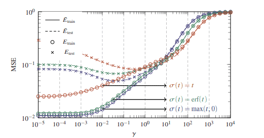
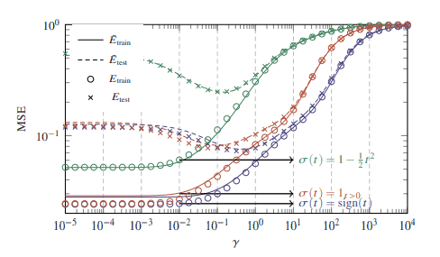
To validate the asymptotic analysis in Theorem $5.1$ and Corollary $5.1$ on real-world data, Figures $5.2$ and $5.3$ compare the empirical MSEs with their limiting behavior predicted in Corollary 5.1, for a random network of $N=512$ neurons and various types of Lipschitz and non-Lipschitz activations $\sigma(\cdot)$, respectively. The regressor $\boldsymbol{\beta} \in \mathbb{R}^p$ maps the vectorized images from the Fashion-MNIST dataset (classes 1 and 2) [Xiao et al., 2017] to their corresponding uni-dimensional ( $d=1$ ) output labels $\mathbf{Y}{1 i}, \hat{\mathbf{Y}}{1 j} \in$ ${\pm 1}$. For $n, p, N$ of order a few hundreds (so not very large when compared to typical modern neural network dimensions), a close match between theory and practice is observed for the Lipschitz activations in Figure 5.2. The precision is less accurate but still quite good for the case of non-Lipschitz activations in Figure 5.3, which, we recall, are formally not supported by the theorem statement – here for $\sigma(t)=1-t^2 / 2$, $\sigma(t)=1_{t>0}$, and $\sigma(t)=\operatorname{sign}(t)$. For all activations, the deviation from theory is more acute for small values of regularization $\gamma$.
Figures $5.2$ and $5.3$ confirm that while the training error is a monotonically increasing function of the regularization parameter $\gamma$, there always exists an optimal value for $\gamma$ which minimizes the test error. In particular, the theoretical formulas derived in Corollary $5.1$ allow for a (data-dependent) fast offline tuning of the hyperparameter $\gamma$ of the network, in the setting where $n, p, N$ are not too small and comparable. In terms of activation functions (those listed here), we observe that, on the Fashion-MNIST dataset, the ReLU nonlinearity $\sigma(t)=\max (t, 0)$ is optimal and achieves the minimum test error, while the quadratic activation $\sigma(t)=1-t^2 / 2$ is the worst and produces much higher training and test errors compared to others. This observation will be theoretically explained through a deeper analysis of the corresponding kernel matrix $\mathbf{K}$, as performed in Section 5.1.2. Lastly, although not immediate at first sight, the training and test error curves of $\sigma(t)=1_{t>0}$ and $\sigma(t)=\operatorname{sign}(t)$ are indeed the same, up to a shift in $\gamma$, as a consequence of the fact that $\operatorname{sign}(t)=2 \cdot 1_{t>0}-1$.
机器学习代考
计算机代写|机器学习代写machine learning代考|Intuition and Main Results
首先考虑训练误差 $E_{\text {train }}$ 在 (5.3) 中定义。自从
$$
\operatorname{tr} \mathbf{Y} \mathbf{Q}^2(\gamma) \mathbf{Y}^{\top}=-\frac{\partial}{\partial \gamma} \operatorname{tr} \mathbf{Y} \mathbf{Q}(\gamma) \mathbf{Y}^{\top}
$$
解决方案的确定性等价物 $\mathbf{Q}(\gamma)$ 足以访问的渐近行为 $E_{\text {train }}$.
线性激活 $\sigma(t)=t$ ,感兴趣的溶剂
$$
\mathbf{Q}(\gamma)=\left(\frac{1}{n} \sigma(\mathbf{W X})^{\top} \sigma(\mathbf{W X})+\gamma \mathbf{I} n\right)^{-1}
$$
与定理 $2.6$ 相同。从某种意义上说,评价 $\mathbf{Q}(\gamma)$ (随后 $E \operatorname{train}$ )要求扩展定理 $2.6$ 处理非线性激活的情 况。现在回想一下,推导出 (线性情况) 的确定性等价物的主要成分
$\mathbf{Q}=\left(\mathbf{X}^{\top} \mathbf{W}^{\top} \mathbf{W X} / n+\gamma \mathbf{I} n\right)^{-1}$ 是我) $\mathbf{X}^{\top} \mathbf{W}^{\top}$ 有 iid 列和 (ii) 它的 $i$ 第 列 $\left[\mathbf{W}^{\top}\right]_i$ 具有独立同分布 (或线性相关) 条目,因此密钥引理 $2.11$ 适用。在线性情况下,由于条目的 iid 属性,这些成立 W. 然 而,对于项目 (i),非线性 $\Sigma^{\top}=\sigma(\mathbf{W X})^{\top}$ 仍然有 iid 列,对于项目 (ii),其 $i$ 第列 $\sigma\left(\left[\mathbf{X}^{\top} \mathbf{W}^{\top}\right] . i\right)$ 不 再具有 iid 或线性相关条目。因此,这里的主要技术难点是获得非线性版本的迹引理,引理 2.11。也就是 说,我们预计尽管应用了逐项非线性 $\sigma$. 这自然落入第 节讨论的测度论的集中 $2.7$ 并由以下引理给出。
引理 $5.1$ (非线性二次型的集中,Louart 等人 [2018,引理 1])。为了 $\mathbf{w} \sim \mathcal{N}\left(\mathbf{0}, \mathbf{I}_p\right)$, 1-利普㹷茨 $\sigma(\cdot)$ ,和 $\mathbf{A} \in \mathbb{R}^{n \times n}, \mathbf{X} \in \mathbb{R}^{p \times n}$ 这样 $|\mathbf{A}| \leq 1$ 和 $|\mathbf{X}|$ 有界于 $p, n$ ,然后,
$$
\mathbb{P}\left(\left|\frac{1}{n} \sigma\left(\mathbf{w}^{\top} \mathbf{X}\right) \mathbf{A} \sigma\left(\mathbf{X}^{\top} \mathbf{w}\right)-\frac{1}{n} \operatorname{tr} \mathbf{A K}\right|>t\right) \leq C e^{-c n \min \left(t, t^2\right)}
$$
对于一些 $C, c>0, p / n \in(0, \infty)$ 和 $^2$
$$
\mathbf{K} \equiv \mathbf{K X X} \equiv \mathbb{E} \mathbf{w} \sim \mathcal{N}\left(\mathbf{0}, \mathbf{I}_p\right)\left[\sigma\left(\mathbf{X}^{\top} \mathbf{w}\right) \sigma\left(\mathbf{w}^{\top} \mathbf{X}\right)\right] \in \mathbb{R}^{n \times n}
$$
计算机代写|机器学习代写machine learning代考|Consequences for Learning with Large Neural Networks
验证定理中的渐近分析5.1和推论 $5.1$ 关于真实世界的数据,数字 $5.2$ 和 $5.3$ 对于一个随机网络,将经验 MSE 与推论 $5.1$ 中预测的限制行为进行比较 $N=512$ 神经元和各种类型的 Lipschitz 和非 Lipschitz 激活 $\sigma(\cdot)$ ,分别。回归者 $\beta \in \mathbb{R}^p$ 将来自 Fashion-MNIST 数据集(第 1 类和第 2 类) [Xiao et al.,2017] 的矢 量化图像映射到它们相应的单维 $(d=1$ ) 输出标签 $\mathbf{Y} 1 i, \hat{\mathbf{Y}} 1 j \in \pm 1$. 为了 $n, p, N$ 数百个数量级 (因此 与典型的现代神经网络维度相比不是很大),在图 $5.2$ 中观察到 Lipschitz 激活的理论与实践之间的紧密 匹配。精度不太准确,但对于图 $5.3$ 中非 Lipschitz 激活的情况仍然相当不错,我们记得,定理陈述正式 不支持这种情况一一这里是为了 $\sigma(t)=1-t^2 / 2 , \sigma(t)=1_{t>0}$ ,和 $\sigma(t)=\operatorname{sign}(t)$. 对于所有激活, 正则化的小值与理论的偏差更为严重 $\gamma$.
数字 $5.2$ 和 $5.3$ 确认虽然训练误差是正则化参数的单调递增函数 $\gamma$ ,总是存在一个最优值 $\gamma$ 从而最小化测试误 差。特别是推论中推导出的理论公式5.1允许对超参数进行 (依赖于数据的) 快速离线调整 $\gamma$ 网络的设置 $n, p, N$ 不是太小且具有可比性。就激活函数(此处列出的那些) 而言,我们观察到,在 Fashion-MNIST 数据集上, $\operatorname{ReLU}$ 非线性 $\sigma(t)=\max (t, 0)$ 是最优的并达到最小测试误差,而二次激活 $\sigma(t)=1-t^2 / 2$ 是最差的,与其他人相比会产生更高的训练和测试错误。将通过对相应核矩阵的更深 入分析从理论上解释这一观察结果 $\mathbf{K}$ ,如第 5.1.2 节中所述。最后,虽然乍一看不是立即的,但训练和测试误差曲线 $\sigma(t)=1_{t>0}$ 和 $\sigma(t)=\operatorname{sign}(t)$ 确实是一样的,直到一个转变 $\gamma$ ,由于这样的事实 $\operatorname{sign}(t)=2 \cdot 1_{t>0}-1$

统计代写请认准statistics-lab™. statistics-lab™为您的留学生涯保驾护航。
金融工程代写
金融工程是使用数学技术来解决金融问题。金融工程使用计算机科学、统计学、经济学和应用数学领域的工具和知识来解决当前的金融问题,以及设计新的和创新的金融产品。
非参数统计代写
非参数统计指的是一种统计方法,其中不假设数据来自于由少数参数决定的规定模型;这种模型的例子包括正态分布模型和线性回归模型。
广义线性模型代考
广义线性模型(GLM)归属统计学领域,是一种应用灵活的线性回归模型。该模型允许因变量的偏差分布有除了正态分布之外的其它分布。
术语 广义线性模型(GLM)通常是指给定连续和/或分类预测因素的连续响应变量的常规线性回归模型。它包括多元线性回归,以及方差分析和方差分析(仅含固定效应)。
有限元方法代写
有限元方法(FEM)是一种流行的方法,用于数值解决工程和数学建模中出现的微分方程。典型的问题领域包括结构分析、传热、流体流动、质量运输和电磁势等传统领域。
有限元是一种通用的数值方法,用于解决两个或三个空间变量的偏微分方程(即一些边界值问题)。为了解决一个问题,有限元将一个大系统细分为更小、更简单的部分,称为有限元。这是通过在空间维度上的特定空间离散化来实现的,它是通过构建对象的网格来实现的:用于求解的数值域,它有有限数量的点。边界值问题的有限元方法表述最终导致一个代数方程组。该方法在域上对未知函数进行逼近。[1] 然后将模拟这些有限元的简单方程组合成一个更大的方程系统,以模拟整个问题。然后,有限元通过变化微积分使相关的误差函数最小化来逼近一个解决方案。
tatistics-lab作为专业的留学生服务机构,多年来已为美国、英国、加拿大、澳洲等留学热门地的学生提供专业的学术服务,包括但不限于Essay代写,Assignment代写,Dissertation代写,Report代写,小组作业代写,Proposal代写,Paper代写,Presentation代写,计算机作业代写,论文修改和润色,网课代做,exam代考等等。写作范围涵盖高中,本科,研究生等海外留学全阶段,辐射金融,经济学,会计学,审计学,管理学等全球99%专业科目。写作团队既有专业英语母语作者,也有海外名校硕博留学生,每位写作老师都拥有过硬的语言能力,专业的学科背景和学术写作经验。我们承诺100%原创,100%专业,100%准时,100%满意。
随机分析代写
随机微积分是数学的一个分支,对随机过程进行操作。它允许为随机过程的积分定义一个关于随机过程的一致的积分理论。这个领域是由日本数学家伊藤清在第二次世界大战期间创建并开始的。
时间序列分析代写
随机过程,是依赖于参数的一组随机变量的全体,参数通常是时间。 随机变量是随机现象的数量表现,其时间序列是一组按照时间发生先后顺序进行排列的数据点序列。通常一组时间序列的时间间隔为一恒定值(如1秒,5分钟,12小时,7天,1年),因此时间序列可以作为离散时间数据进行分析处理。研究时间序列数据的意义在于现实中,往往需要研究某个事物其随时间发展变化的规律。这就需要通过研究该事物过去发展的历史记录,以得到其自身发展的规律。
回归分析代写
多元回归分析渐进(Multiple Regression Analysis Asymptotics)属于计量经济学领域,主要是一种数学上的统计分析方法,可以分析复杂情况下各影响因素的数学关系,在自然科学、社会和经济学等多个领域内应用广泛。
MATLAB代写
MATLAB 是一种用于技术计算的高性能语言。它将计算、可视化和编程集成在一个易于使用的环境中,其中问题和解决方案以熟悉的数学符号表示。典型用途包括:数学和计算算法开发建模、仿真和原型制作数据分析、探索和可视化科学和工程图形应用程序开发,包括图形用户界面构建MATLAB 是一个交互式系统,其基本数据元素是一个不需要维度的数组。这使您可以解决许多技术计算问题,尤其是那些具有矩阵和向量公式的问题,而只需用 C 或 Fortran 等标量非交互式语言编写程序所需的时间的一小部分。MATLAB 名称代表矩阵实验室。MATLAB 最初的编写目的是提供对由 LINPACK 和 EISPACK 项目开发的矩阵软件的轻松访问,这两个项目共同代表了矩阵计算软件的最新技术。MATLAB 经过多年的发展,得到了许多用户的投入。在大学环境中,它是数学、工程和科学入门和高级课程的标准教学工具。在工业领域,MATLAB 是高效研究、开发和分析的首选工具。MATLAB 具有一系列称为工具箱的特定于应用程序的解决方案。对于大多数 MATLAB 用户来说非常重要,工具箱允许您学习和应用专业技术。工具箱是 MATLAB 函数(M 文件)的综合集合,可扩展 MATLAB 环境以解决特定类别的问题。可用工具箱的领域包括信号处理、控制系统、神经网络、模糊逻辑、小波、仿真等。