如果你也在 怎样代写数学建模Mathematical Modeling这个学科遇到相关的难题,请随时右上角联系我们的24/7代写客服。数学建模Mathematical Modeling最好是通过制作数学模型来学习的。为实现这一目标,已编制了三种类型的演习。其中一些进一步发展了文中给出的模型;另一些要求读者改变文中给出的模型的假设,然后,推断新模型的结果,并与新情况的结果进行比较。
数学建模Mathematical Modeling都是从物理、生物、社会、经济、管理和工程科学中选择的。这些模型处理不同的概念,但具有共同的数学结构,并体现了不同学科数学建模的统一影响。因此,物理学、生物学、经济学、心理学和工程学中完全不同的问题可以用一个共同的数学模型来表示。模型是一样的;只是解释不同而已。当不同的技术是最合适的时候,努力解释概念。
statistics-lab™ 为您的留学生涯保驾护航 在代写数学建模math modelling方面已经树立了自己的口碑, 保证靠谱, 高质且原创的统计Statistics代写服务。我们的专家在代写数学建模math modelling代写方面经验极为丰富,各种代写数学建模math modelling相关的作业也就用不着说。

数学代写|数学建模代写math modelling代考|Econodynamics: An Information-theoretic Model for Economics
Let $c_{1, c 2, \ldots, c n}$ be the costs of travel from $n$ suburbs to the central business district and let the average travel budget $\sum_{i=1}^n p_i c_i=\bar{c}$ be known, then to estimate the proportions $p_1, p_2, \ldots, p_n$ of the population living in these suburbs, we maximize the entropy $-\sum_{i=1}^n p_i \ln p_i$ subject to $\sum_{i=1}^n p_i=1$ and $\sum_{i=1}^{\mathrm{n}} p_i c_i=\bar{c}$ to get
$$
p_i=\exp \left(-\mu c_i\right) / \sum_{i=1}^n \exp \left(-\mu c_i\right), i=1,2, \ldots, n
$$
which is the Maxwell-Boltzmann distribution and we can proceed as in Section 10.4.1 to define an economic temperature $T=1 / \mu \bar{c}$, an economic heat $\Delta H=\sum_{i=1}^n c_i d p_i$ and an economic entropy by $d S_{\max }=\sum_{i=1}^n c_i d p_i / T$. From $(89)$
$$
S_{\max }=\mu \bar{c}+\ln \sum_{i=1}^n \exp \left(-\mu c_i\right)
$$
Keeping $c_1, c_2, \ldots, c_n$ fixed, $S_{\max }$ is a function of $\bar{c}$ and
$$
\begin{aligned}
& \frac{d S_{\max }}{d \bar{c}}=\mu+\bar{c} \frac{d \mu}{d c}+\frac{\sum_{i=1}^n \exp \left(-\mu c_i\right)\left(-c_i \frac{d \mu}{d c}\right)}{\sum_{i=1}^n \exp \left(-\mu c_i\right)} \
&=\mu+\bar{c} \frac{d \mu}{d c}-\bar{c} \frac{d \mu}{d \bar{c}}=\mu \
& \frac{d^2 S_{\max }}{d \bar{c}^2}=\frac{d \mu}{d \bar{c}} \
&=\frac{\left(\sum_{i=1}^n \exp \left(-\mu c_i\right)\right)^2}{\left(\sum_{i=1}^n \mu_i \exp \left(-\mu c_i\right)\right)^2-\left(\sum_{i=1}^n \exp \left(-\mu c_i\right)\right)\left(\sum_{i=1}^n c_1^2 \exp \left(-\mu c_i\right)\right)^2} \leq 0
\end{aligned}
$$
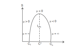
so that $S_{\max }$ is a concave function of $\bar{c}$. If we arrange $c_1, c_2, \ldots, c_n$ in ascending order then when
$$
\bar{c}=c_1, p_1=1, p_2=0, \ldots, p_n=0 \text { and } S=0
$$
when
$$
\bar{c}=c_n, p_1=1, p_2=0, \ldots, p_n=1 \text { and } S=0
$$
and
$$
\bar{c}=c^{\circ}=\frac{1}{n}\left(c_1+c_2+\ldots+c_n\right), p_1=p_2=\ldots=p_n=\frac{1}{n}
$$
and
$$
S=\ln n
$$
数学代写|数学建模代写math modelling代考|Gravity Model for Transportation Problem in Urban and Regional Planning
There are $m$ residential suburbs $A_1, A_2, \ldots, A_m$ in which $a_1 a_2, \ldots, a_m$ office workers live and there are $n$ offices $B_1, B_2, \ldots, B_n$ in which $b_1, b_2, \ldots, b_n$ workers work so that
$$
\sum_{i=1}^m a_i=\sum_{j=1}^n b_j=T
$$
where $T$ is the total number of office workers in all the suburbs. Let $T_{i j}$ be the number of workers traveling from the $i$ th residential suburb to the $j$ th office so that
$$
\sum_{j=1}^n T_{i j}=a_i, \sum_{i=1}^m T_{i j}=b_j
$$
Equations (119) and (120) give $m+n-1$ equations to determine $m n$ unknown quantities of $T_{i j}$ ‘s $(i=1,2, \ldots, m ; j=1,2, \ldots, n)$. Obviously these equations are not sufficient to determine $T_{i j}$ ‘s uniquely and we appeal to the principle of maximum entropy. We maximize the entropy
$$
S=-\sum_{i=1}^m \sum_{j=1}^n \frac{T_{i j}}{T} \ln \frac{T_{i j}}{T}
$$
subject to Eqns. (119) and (120) and the cost constraint.
$$
\sum_{i=1}^m \sum_{j=1}^n T_{i j} c_{i j}=\bar{c}
$$
to get
$$
T_{i j}=A_i B_j a_i b_j \exp \left(-v c_{i j}\right)
$$
The constants $A_i(i=1,2, \ldots, m), B_j(j=1,2, \ldots, n)$, and $v$ can be determined by using Eqns. (119), (120), and (122).
This method is called the gravity model of transportation since (123) was deduced by starting from
$$
T_{i j}=K \frac{a_i b_i}{c_{i j}^2}
$$
on the analogy of Newton’s laws of gravitation and then modifying it empirically over a period of thirty years to make it consistent mathematically and with observations. The formula which took thirty years to develop empirically and by trial and error could be deduced in a straightforward manner by using mathematical modeling through the maximum entropy principle.
数学建模代写
数学代写|数学建模代写math modelling代考|Econodynamics: An Information-theoretic Model for Economics
设$c_{1, c 2, \ldots, c n}$为从$n$郊区到中央商务区的旅行成本,并设平均旅行预算$\sum_{i=1}^n p_i c_i=\bar{c}$为已知,则为了估计居住在这些郊区的人口比例$p_1, p_2, \ldots, p_n$,我们将熵$-\sum_{i=1}^n p_i \ln p_i$最大化,服从$\sum_{i=1}^n p_i=1$和$\sum_{i=1}^{\mathrm{n}} p_i c_i=\bar{c}$得到
$$
p_i=\exp \left(-\mu c_i\right) / \sum_{i=1}^n \exp \left(-\mu c_i\right), i=1,2, \ldots, n
$$
这就是麦克斯韦-玻尔兹曼分布,我们可以像第10.4.1节那样继续定义经济温度$T=1 / \mu \bar{c}$,经济热$\Delta H=\sum_{i=1}^n c_i d p_i$和经济熵$d S_{\max }=\sum_{i=1}^n c_i d p_i / T$。来自$(89)$
$$
S_{\max }=\mu \bar{c}+\ln \sum_{i=1}^n \exp \left(-\mu c_i\right)
$$
保持$c_1, c_2, \ldots, c_n$不变,$S_{\max }$是$\bar{c}$和的函数
$$
\begin{aligned}
& \frac{d S_{\max }}{d \bar{c}}=\mu+\bar{c} \frac{d \mu}{d c}+\frac{\sum_{i=1}^n \exp \left(-\mu c_i\right)\left(-c_i \frac{d \mu}{d c}\right)}{\sum_{i=1}^n \exp \left(-\mu c_i\right)} \
&=\mu+\bar{c} \frac{d \mu}{d c}-\bar{c} \frac{d \mu}{d \bar{c}}=\mu \
& \frac{d^2 S_{\max }}{d \bar{c}^2}=\frac{d \mu}{d \bar{c}} \
&=\frac{\left(\sum_{i=1}^n \exp \left(-\mu c_i\right)\right)^2}{\left(\sum_{i=1}^n \mu_i \exp \left(-\mu c_i\right)\right)^2-\left(\sum_{i=1}^n \exp \left(-\mu c_i\right)\right)\left(\sum_{i=1}^n c_1^2 \exp \left(-\mu c_i\right)\right)^2} \leq 0
\end{aligned}
$$
所以$S_{\max }$是$\bar{c}$的凹函数。如果我们将$c_1, c_2, \ldots, c_n$按升序排列,那么当
$$
\bar{c}=c_1, p_1=1, p_2=0, \ldots, p_n=0 \text { and } S=0
$$
什么时候
$$
\bar{c}=c_n, p_1=1, p_2=0, \ldots, p_n=1 \text { and } S=0
$$
和
$$
\bar{c}=c^{\circ}=\frac{1}{n}\left(c_1+c_2+\ldots+c_n\right), p_1=p_2=\ldots=p_n=\frac{1}{n}
$$
和
$$
S=\ln n
$$
数学代写|数学建模代写math modelling代考|Gravity Model for Transportation Problem in Urban and Regional Planning
有$m$住宅郊区$A_1, A_2, \ldots, A_m$, $a_1 a_2, \ldots, a_m$上班族住在那里,有$n$办公室$B_1, B_2, \ldots, B_n$, $b_1, b_2, \ldots, b_n$上班族在那里工作
$$
\sum_{i=1}^m a_i=\sum_{j=1}^n b_j=T
$$
其中$T$是所有郊区上班族的总数。设$T_{i j}$为从$i$第一个住宅区到$j$第一个办公室的工人人数,以便
$$
\sum_{j=1}^n T_{i j}=a_i, \sum_{i=1}^m T_{i j}=b_j
$$
式(119)和式(120)给出了$m+n-1$方程来确定$T_{i j}$的$(i=1,2, \ldots, m ; j=1,2, \ldots, n)$的$m n$未知量。显然,这些方程不足以唯一地确定$T_{i j}$的s,我们求助于最大熵原理。我们最大化熵
$$
S=-\sum_{i=1}^m \sum_{j=1}^n \frac{T_{i j}}{T} \ln \frac{T_{i j}}{T}
$$
受法律约束。(119)和(120)以及成本约束。
$$
\sum_{i=1}^m \sum_{j=1}^n T_{i j} c_{i j}=\bar{c}
$$
为了得到
$$
T_{i j}=A_i B_j a_i b_j \exp \left(-v c_{i j}\right)
$$
常数$A_i(i=1,2, \ldots, m), B_j(j=1,2, \ldots, n)$和$v$可以通过使用Eqns确定。(119),(120),(122)。
这种方法被称为运输重力模型,因为(123)是从
$$
T_{i j}=K \frac{a_i b_i}{c_{i j}^2}
$$
在牛顿万有引力定律的类比上,然后在30年的时间里对它进行了经验修改,使它在数学上和观测上一致。这个公式是用了三十年的经验和反复试验得出的,可以通过最大熵原理建立数学模型,以一种直观的方式推导出来。

统计代写请认准statistics-lab™. statistics-lab™为您的留学生涯保驾护航。
金融工程代写
金融工程是使用数学技术来解决金融问题。金融工程使用计算机科学、统计学、经济学和应用数学领域的工具和知识来解决当前的金融问题,以及设计新的和创新的金融产品。
非参数统计代写
非参数统计指的是一种统计方法,其中不假设数据来自于由少数参数决定的规定模型;这种模型的例子包括正态分布模型和线性回归模型。
广义线性模型代考
广义线性模型(GLM)归属统计学领域,是一种应用灵活的线性回归模型。该模型允许因变量的偏差分布有除了正态分布之外的其它分布。
术语 广义线性模型(GLM)通常是指给定连续和/或分类预测因素的连续响应变量的常规线性回归模型。它包括多元线性回归,以及方差分析和方差分析(仅含固定效应)。
有限元方法代写
有限元方法(FEM)是一种流行的方法,用于数值解决工程和数学建模中出现的微分方程。典型的问题领域包括结构分析、传热、流体流动、质量运输和电磁势等传统领域。
有限元是一种通用的数值方法,用于解决两个或三个空间变量的偏微分方程(即一些边界值问题)。为了解决一个问题,有限元将一个大系统细分为更小、更简单的部分,称为有限元。这是通过在空间维度上的特定空间离散化来实现的,它是通过构建对象的网格来实现的:用于求解的数值域,它有有限数量的点。边界值问题的有限元方法表述最终导致一个代数方程组。该方法在域上对未知函数进行逼近。[1] 然后将模拟这些有限元的简单方程组合成一个更大的方程系统,以模拟整个问题。然后,有限元通过变化微积分使相关的误差函数最小化来逼近一个解决方案。
tatistics-lab作为专业的留学生服务机构,多年来已为美国、英国、加拿大、澳洲等留学热门地的学生提供专业的学术服务,包括但不限于Essay代写,Assignment代写,Dissertation代写,Report代写,小组作业代写,Proposal代写,Paper代写,Presentation代写,计算机作业代写,论文修改和润色,网课代做,exam代考等等。写作范围涵盖高中,本科,研究生等海外留学全阶段,辐射金融,经济学,会计学,审计学,管理学等全球99%专业科目。写作团队既有专业英语母语作者,也有海外名校硕博留学生,每位写作老师都拥有过硬的语言能力,专业的学科背景和学术写作经验。我们承诺100%原创,100%专业,100%准时,100%满意。
随机分析代写
随机微积分是数学的一个分支,对随机过程进行操作。它允许为随机过程的积分定义一个关于随机过程的一致的积分理论。这个领域是由日本数学家伊藤清在第二次世界大战期间创建并开始的。
时间序列分析代写
随机过程,是依赖于参数的一组随机变量的全体,参数通常是时间。 随机变量是随机现象的数量表现,其时间序列是一组按照时间发生先后顺序进行排列的数据点序列。通常一组时间序列的时间间隔为一恒定值(如1秒,5分钟,12小时,7天,1年),因此时间序列可以作为离散时间数据进行分析处理。研究时间序列数据的意义在于现实中,往往需要研究某个事物其随时间发展变化的规律。这就需要通过研究该事物过去发展的历史记录,以得到其自身发展的规律。
回归分析代写
多元回归分析渐进(Multiple Regression Analysis Asymptotics)属于计量经济学领域,主要是一种数学上的统计分析方法,可以分析复杂情况下各影响因素的数学关系,在自然科学、社会和经济学等多个领域内应用广泛。
MATLAB代写
MATLAB 是一种用于技术计算的高性能语言。它将计算、可视化和编程集成在一个易于使用的环境中,其中问题和解决方案以熟悉的数学符号表示。典型用途包括:数学和计算算法开发建模、仿真和原型制作数据分析、探索和可视化科学和工程图形应用程序开发,包括图形用户界面构建MATLAB 是一个交互式系统,其基本数据元素是一个不需要维度的数组。这使您可以解决许多技术计算问题,尤其是那些具有矩阵和向量公式的问题,而只需用 C 或 Fortran 等标量非交互式语言编写程序所需的时间的一小部分。MATLAB 名称代表矩阵实验室。MATLAB 最初的编写目的是提供对由 LINPACK 和 EISPACK 项目开发的矩阵软件的轻松访问,这两个项目共同代表了矩阵计算软件的最新技术。MATLAB 经过多年的发展,得到了许多用户的投入。在大学环境中,它是数学、工程和科学入门和高级课程的标准教学工具。在工业领域,MATLAB 是高效研究、开发和分析的首选工具。MATLAB 具有一系列称为工具箱的特定于应用程序的解决方案。对于大多数 MATLAB 用户来说非常重要,工具箱允许您学习和应用专业技术。工具箱是 MATLAB 函数(M 文件)的综合集合,可扩展 MATLAB 环境以解决特定类别的问题。可用工具箱的领域包括信号处理、控制系统、神经网络、模糊逻辑、小波、仿真等。