如果你也在 怎样代写力学mechanics这个学科遇到相关的难题,请随时右上角联系我们的24/7代写客服。
力学是物理学的一个分支,主要研究能量和力以及它们与物体的平衡、变形或运动的关系。
statistics-lab™ 为您的留学生涯保驾护航 在代写力学mechanics方面已经树立了自己的口碑, 保证靠谱, 高质且原创的统计Statistics代写服务。我们的专家在代写力学mechanics代写方面经验极为丰富,各种代写力学mechanics相关的作业也就用不着说。
我们提供的力学mechanics及其相关学科的代写,服务范围广, 其中包括但不限于:
- Statistical Inference 统计推断
- Statistical Computing 统计计算
- Advanced Probability Theory 高等概率论
- Advanced Mathematical Statistics 高等数理统计学
- (Generalized) Linear Models 广义线性模型
- Statistical Machine Learning 统计机器学习
- Longitudinal Data Analysis 纵向数据分析
- Foundations of Data Science 数据科学基础
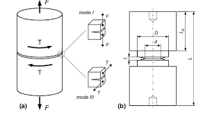
物理代写|力学代写mechanics代考|Opening-Mode Loading
Consider a transparent specimen illuminated by a parallel light beam and a screen at a distance $z_0$ downstream from the specimen placed parallel to the plane of the specimen (Fig. 6.9). A point $P$ on the specimen is imaged at point $P^{\prime}$ on the screen. It is assumed that the slopes of the surface are small and the distance $z_0$ is large compared to the change of the specimen thickness due to loading.
For the case of a transparent specimen the mapping equation of point $P$ to point $P^{\prime}$, according to Eq. $(6.5)$, is given by
$$
\begin{aligned}
& W_x=x-z_0 \frac{\partial(\Delta s)}{\partial x} \
& W_y=y-z_0 \frac{\partial(\Delta s)}{\partial y}
\end{aligned}
$$
where $\Delta s$ is the change of the optical path of a ray passing through the specimen due to loading.
For an optically inert material, $\Delta s$ is given by Eq. (6.37) for the light rays traversing the specimen and by Eq. (6.44) for the light rays reflected from the rear face of the transparent specimen. For the rays reflected from the front face of the specimen the stress-optical constant $c_t$ in Eq. (6.37) should be replaced by the ratio $v / E(v$ is the Poisson’s ratio and $E$ is the modulus of elasticity). For all three cases of light rays traversing the specimen, reflected from the rear face or from the front face of the specimen the transformation Fq. (6.45) applies with different valnes of the stress-optical constant $\mathrm{c}$, which takes the values $c_t, 2 c_r$, or $v / E$, respectively.
The singular polar stresses at the tip of the crack for opening-mode loading governed by value of the stress intensity factor $K_I$ are given by [2]
$$
\begin{aligned}
\sigma_r & =\frac{K_I}{4 \sqrt{2 \pi r}}\left(5 \cos \frac{\theta}{2}-\cos \frac{3 \theta}{2}\right) \
\sigma_\theta & =\frac{K_I}{4 \sqrt{2 \pi r}}\left(3 \cos \frac{\theta}{2}+\cos \frac{3 \theta}{2}\right) \
\sigma_{r \theta} & =\frac{K_I}{4 \sqrt{2 \pi r}}\left(\sin \frac{\theta}{2}+\sin \frac{3 \theta}{2}\right)
\end{aligned}
$$
where $r$ is the distance from the origin of the coordinate system placed at the crack tip and $\theta$ is the polar angle.
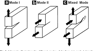
物理代写|力学代写mechanics代考|Mixed-Mode Loading
When the applied loads are not normal to the crack plane mixed-mode conditions apply in the vicinity of the crack tip. The singular stresses in polar coordinates are given in terms of the opening-mode $K_I$ and sliding-mode $K_{I I}$ stress intensity factors by the following equations [2]
$$
\begin{aligned}
\sigma_r & =\frac{K_I}{4 \sqrt{2 \pi r}}\left(5 \cos \frac{\theta}{2}-\cos \frac{3 \theta}{2}\right)+\frac{K_{I I}}{4 \sqrt{2 \pi r}}\left(-5 \sin \frac{\theta}{2}+3 \sin \frac{3 \theta}{2}\right) \
\sigma_\theta & =\frac{K_I}{4 \sqrt{2 \pi r}}\left(3 \cos \frac{\theta}{2}+\cos \frac{3 \theta}{2}\right)+\frac{K_{I I}}{4 \sqrt{2 \pi r}}\left(-3 \sin \frac{\theta}{2}-3 \sin \frac{3 \theta}{2}\right)
\end{aligned}
$$ $$
\sigma_{r \theta}=\frac{K_I}{4 \sqrt{2 \pi r}}\left(\sin \frac{\theta}{2}+\sin \frac{3 \theta}{2}\right)+\frac{K_{I I}}{4 \sqrt{2 \pi r}}\left(\cos \frac{\theta}{2}+3 \cos \frac{3 \theta}{2}\right)
$$
The sum of the stresses $\sigma_r$ and $\sigma_\theta$ is given by
$$
\sigma_r+\sigma_\theta=\frac{2 K_I}{\sqrt{2 \pi r}} \cos \frac{\theta}{2}-\frac{2 K_{I I}}{\sqrt{2 \pi r}} \sin \frac{\theta}{2}
$$
Working as in the previous case of opening-mode loading, we obtain the following equations of the caustic
$$
\begin{aligned}
& W_x=x^{\prime}=r_0\left[\cos \theta+\frac{2}{3}\left(1+\mu^2\right)^{-1 / 2} \cos \frac{3 \theta}{2}-\frac{2}{3} \mu\left(1+\mu^2\right)^{-1 / 2} \sin \frac{3 \theta}{2}\right] \
& W_y=y^{\prime}=r_0\left[\sin \theta+\frac{2}{3}\left(1+\mu^2\right)^{-1 / 2} \sin \frac{3 \theta}{2}+\frac{2}{3} \mu\left(1+\mu^2\right)^{-1 / 2} \cos \frac{3 \theta}{2}\right]
\end{aligned}
$$
With
$$
r=r_0=\left(\frac{3 z_0 d c K_I}{2 \sqrt{2 \pi}}\right)^{2 / 5}\left(1+\mu^2\right)^{1 / 5}, \quad \mu=K_{I I} / K_I
$$
The stress intensity factors $K_I$ and $K_{I I}$ are obtained as
$$
K_I=\frac{1.671}{z_0 d c m^{3 / 2}}\left(\frac{D}{\delta}\right)^{5 / 2} \frac{1}{\sqrt{1+\mu^2}}, \quad K_{I I}=\mu K_I
$$
The ratio $D / \delta$ takes either of the values $r_0=D_t / \delta_t, D_l^{\max } / \delta_l^{\max }, D_l^{\min } / \delta_l^{\min }$, where $D_l^{\max }$ and $D_l^{\min }$ are the maximum and minimum diameters of the caustic along the cräck planee and $D_t$ is the transverse (perpendiculär to the crack plané) dianeter of the caustic at the crack tip. The quantities $\delta_l^{\max }$ and $\delta_l^{\min }$ depend on the value of 4. For opening-mode loading $\delta_t=3.16, \delta_l^{\max }=\delta_l^{\min }=3$. Figure 6.13 presents the geometrical construction of the caustic for $\mu=0.5$. In Fig. 6.14 four caustics corresponding to $\mu=0,0.25,1.0$ and $\infty$ are shown. The values of $\mu=0$ and $\infty$ refer to the cases of pure tension (opening-mode loading) and pure shear (sliding-mode loading), respectively. Note that the caustic for $\mu=0$ is symmetric with respect to the $x$-axis, while the other caustics for $\mu \neq 0$ do not present a symmetry. Figure 6.15 presents the variation of the quantities $\delta_t=D_t / r_0, \delta_l^{\max }=D_l^{\max } / r_0, \delta_l^{\min }=D_l^{\min } / r_0$ versus $\mu$. Note that for $\mu=0 . \delta_t=3.16$, while for $\mu=1, \delta_t=2.99$. The variation of the ratio $\left(D_l^{\max }-D_l^{\min }\right) / D_l^{\max }$ versus $\mu$ is shown in Fig. 6.16.
力学代考
物理代写|力学代写mechanics代考|Opening-Mode Loading
考虑一个由平行光束和远处的屏幕照亮的透明标本 $z_0$ 样品下游平行于样品平面放置 (图 6.9) 。一点 $P$ 标本上的成像点 $P^{\prime}$ 屏幕上。假设表面的斜率很小并且距离 $z_0$ 与载荷引起的试样厚度变化相比,它很大。
对于透明样品的情况,点的映射方程 $P$ 指向 $P^{\prime}$ ,根据方程式。 (6.5),是(谁) 给的
$$
W_x=x-z_0 \frac{\partial(\Delta s)}{\partial x} \quad W_y=y-z_0 \frac{\partial(\Delta s)}{\partial y}
$$
在哪里 $\Delta s$ 是由于载荷引起的穿过试样的光线光路的变化。
对于光学惰性材料, $\Delta s$ 由方程式给出。(6.37) 对于穿过样品的光线和通过 Eq. (6.44) 对于从透明样品背 面反射的光线。对于从试样正面反射的光线,应力光学常数 $c_t$ 在等式中 (6.37) 应替换为比率 $v / E(v$ 是泊 松比和 $E$ 是弹性模量)。对于穿过样本的所有三种情况,从样本的背面或从样本的正面反射的变换 $F q$ 。 (6.45) 适用于应力光学常数的不同值c, 它取值 $c_t, 2 c_r$ ,或者 $v / E$ ,分别。
由应力强度因子的值控制的开模加载裂纹尖端的奇异极性应力 $K_I$ 由 [2] 给出
$$
\sigma_r=\frac{K_I}{4 \sqrt{2 \pi r}}\left(5 \cos \frac{\theta}{2}-\cos \frac{3 \theta}{2}\right) \sigma_\theta=\frac{K_I}{4 \sqrt{2 \pi r}}\left(3 \cos \frac{\theta}{2}+\cos \frac{3 \theta}{2}\right) \sigma_{r \theta}=\frac{K_I}{4 \sqrt{2 \pi r}}(\sin
$$
在哪里 $r$ 是距位于裂纹尖端的坐标系原点的距离, $\theta$ 是极角。
物理代写|力学代写mechanics代考|Mixed-Mode Loading
当施加的载荷不垂直于裂纹平面时,混合模式条件适用于裂纹尖端附近。极坐标中的奇异应力以开模形 式给出 $K_I$ 和滑动模式 $K_{I I}$ 应力强度因子由以下方程 [2]
$$
\begin{gathered}
\sigma_r=\frac{K_I}{4 \sqrt{2 \pi r}}\left(5 \cos \frac{\theta}{2}-\cos \frac{3 \theta}{2}\right)+\frac{K_{I I}}{4 \sqrt{2 \pi r}}\left(-5 \sin \frac{\theta}{2}+3 \sin \frac{3 \theta}{2}\right) \sigma_\theta=\frac{K_I}{4 \sqrt{2 \pi r}}(3 \cos \
\sigma_{r \theta}=\frac{K_I}{4 \sqrt{2 \pi r}}\left(\sin \frac{\theta}{2}+\sin \frac{3 \theta}{2}\right)+\frac{K_{I I}}{4 \sqrt{2 \pi r}}\left(\cos \frac{\theta}{2}+3 \cos \frac{3 \theta}{2}\right)
\end{gathered}
$$
应力总和 $\sigma_r$ 和 $\sigma_\theta$ 是 (谁) 给的
$$
\sigma_r+\sigma_\theta=\frac{2 K_I}{\sqrt{2 \pi r}} \cos \frac{\theta}{2}-\frac{2 K_{I I}}{\sqrt{2 \pi r}} \sin \frac{\theta}{2}
$$
与前面的开放模式加载情况一样,我们得到以下焦散方程
$$
W_x=x^{\prime}=r_0\left[\cos \theta+\frac{2}{3}\left(1+\mu^2\right)^{-1 / 2} \cos \frac{3 \theta}{2}-\frac{2}{3} \mu\left(1+\mu^2\right)^{-1 / 2} \sin \frac{3 \theta}{2}\right] \quad W_y=y^{\prime}=r_0
$$
和
$$
r=r_0=\left(\frac{3 z_0 d c K_I}{2 \sqrt{2 \pi}}\right)^{2 / 5}\left(1+\mu^2\right)^{1 / 5}, \quad \mu=K_{I I} / K_I
$$
应力强度因子 $K_I$ 和 $K_{I I}$ 获得为
$$
K_I=\frac{1.671}{z_0 d c m^{3 / 2}}\left(\frac{D}{\delta}\right)^{5 / 2} \frac{1}{\sqrt{1+\mu^2}}, \quad K_{I I}=\mu K_I
$$
比例 $D / \delta$ 取任一个值 $r_0=D_t / \delta_t, D_l^{\max } / \delta_l^{\max }, D_l^{\min } / \delta_l^{\min }$ ,在哪里 $D_l^{\max }$ 和 $D_l^{\min }$ 是焦散沿裂纹平 面的最大和最小直径,并且 $D_t$ 是裂纹尖端焦散的横向 (垂直于裂纹平面) 直径。数量 $\delta_l^{\max }$ 和 $\delta_l^{\min }$ 取决 于4的值。对于开放模式加载 $\delta_t=3.16, \delta_l^{\max }=\delta_l^{\min }=3$. 图 6.13 展示了焦散的几何构造 $\mu=0.5$. 在图 6.14 中,四个焦散对应于 $\mu=0,0.25,1.0$ 和 $\infty$ 显示。的价值观 $\mu=0$ 和 $\infty$ 分别指纯张力(开模 加载) 和纯剪切 (滑模加载) 的情况。请注意,苛性碱 $\mu=0$ 是关于对称的 $x$-轴,而其他焦散 $\mu \neq 0$ 不 呈现对称性。图 6.15 显示了数量的变化 $\delta_t=D_t / r_0, \delta_l^{\max }=D_l^{\max } / r_0, \delta_l^{\min }=D_l^{\min } / r_0$ 相对 $\mu$. 请 注意,对于 $\mu=0 . \delta_t=3.16$, 而对于 $\mu=1, \delta_t=2.99$. 比率的变化 $\left(D_l^{\max }-D_l^{\min }\right) / D_l^{\max }$ 相对 $\mu$ 如图 6.16 所示。

统计代写请认准statistics-lab™. statistics-lab™为您的留学生涯保驾护航。
金融工程代写
金融工程是使用数学技术来解决金融问题。金融工程使用计算机科学、统计学、经济学和应用数学领域的工具和知识来解决当前的金融问题,以及设计新的和创新的金融产品。
非参数统计代写
非参数统计指的是一种统计方法,其中不假设数据来自于由少数参数决定的规定模型;这种模型的例子包括正态分布模型和线性回归模型。
广义线性模型代考
广义线性模型(GLM)归属统计学领域,是一种应用灵活的线性回归模型。该模型允许因变量的偏差分布有除了正态分布之外的其它分布。
术语 广义线性模型(GLM)通常是指给定连续和/或分类预测因素的连续响应变量的常规线性回归模型。它包括多元线性回归,以及方差分析和方差分析(仅含固定效应)。
有限元方法代写
有限元方法(FEM)是一种流行的方法,用于数值解决工程和数学建模中出现的微分方程。典型的问题领域包括结构分析、传热、流体流动、质量运输和电磁势等传统领域。
有限元是一种通用的数值方法,用于解决两个或三个空间变量的偏微分方程(即一些边界值问题)。为了解决一个问题,有限元将一个大系统细分为更小、更简单的部分,称为有限元。这是通过在空间维度上的特定空间离散化来实现的,它是通过构建对象的网格来实现的:用于求解的数值域,它有有限数量的点。边界值问题的有限元方法表述最终导致一个代数方程组。该方法在域上对未知函数进行逼近。[1] 然后将模拟这些有限元的简单方程组合成一个更大的方程系统,以模拟整个问题。然后,有限元通过变化微积分使相关的误差函数最小化来逼近一个解决方案。
tatistics-lab作为专业的留学生服务机构,多年来已为美国、英国、加拿大、澳洲等留学热门地的学生提供专业的学术服务,包括但不限于Essay代写,Assignment代写,Dissertation代写,Report代写,小组作业代写,Proposal代写,Paper代写,Presentation代写,计算机作业代写,论文修改和润色,网课代做,exam代考等等。写作范围涵盖高中,本科,研究生等海外留学全阶段,辐射金融,经济学,会计学,审计学,管理学等全球99%专业科目。写作团队既有专业英语母语作者,也有海外名校硕博留学生,每位写作老师都拥有过硬的语言能力,专业的学科背景和学术写作经验。我们承诺100%原创,100%专业,100%准时,100%满意。
随机分析代写
随机微积分是数学的一个分支,对随机过程进行操作。它允许为随机过程的积分定义一个关于随机过程的一致的积分理论。这个领域是由日本数学家伊藤清在第二次世界大战期间创建并开始的。
时间序列分析代写
随机过程,是依赖于参数的一组随机变量的全体,参数通常是时间。 随机变量是随机现象的数量表现,其时间序列是一组按照时间发生先后顺序进行排列的数据点序列。通常一组时间序列的时间间隔为一恒定值(如1秒,5分钟,12小时,7天,1年),因此时间序列可以作为离散时间数据进行分析处理。研究时间序列数据的意义在于现实中,往往需要研究某个事物其随时间发展变化的规律。这就需要通过研究该事物过去发展的历史记录,以得到其自身发展的规律。
回归分析代写
多元回归分析渐进(Multiple Regression Analysis Asymptotics)属于计量经济学领域,主要是一种数学上的统计分析方法,可以分析复杂情况下各影响因素的数学关系,在自然科学、社会和经济学等多个领域内应用广泛。
MATLAB代写
MATLAB 是一种用于技术计算的高性能语言。它将计算、可视化和编程集成在一个易于使用的环境中,其中问题和解决方案以熟悉的数学符号表示。典型用途包括:数学和计算算法开发建模、仿真和原型制作数据分析、探索和可视化科学和工程图形应用程序开发,包括图形用户界面构建MATLAB 是一个交互式系统,其基本数据元素是一个不需要维度的数组。这使您可以解决许多技术计算问题,尤其是那些具有矩阵和向量公式的问题,而只需用 C 或 Fortran 等标量非交互式语言编写程序所需的时间的一小部分。MATLAB 名称代表矩阵实验室。MATLAB 最初的编写目的是提供对由 LINPACK 和 EISPACK 项目开发的矩阵软件的轻松访问,这两个项目共同代表了矩阵计算软件的最新技术。MATLAB 经过多年的发展,得到了许多用户的投入。在大学环境中,它是数学、工程和科学入门和高级课程的标准教学工具。在工业领域,MATLAB 是高效研究、开发和分析的首选工具。MATLAB 具有一系列称为工具箱的特定于应用程序的解决方案。对于大多数 MATLAB 用户来说非常重要,工具箱允许您学习和应用专业技术。工具箱是 MATLAB 函数(M 文件)的综合集合,可扩展 MATLAB 环境以解决特定类别的问题。可用工具箱的领域包括信号处理、控制系统、神经网络、模糊逻辑、小波、仿真等。