如果你也在 怎样代写微观经济学Microeconomics这个学科遇到相关的难题,请随时右上角联系我们的24/7代写客服。
微观经济学是研究稀缺性及其对资源的使用、商品和服务的生产、生产和福利的长期增长的影响,以及对社会至关重要的其他大量复杂问题的研究。
statistics-lab™ 为您的留学生涯保驾护航 在代写微观经济学Microeconomics方面已经树立了自己的口碑, 保证靠谱, 高质且原创的统计Statistics代写服务。我们的专家在代写微观经济学Microeconomics代写方面经验极为丰富,各种代写微观经济学Microeconomics相关的作业也就用不着说。
我们提供的微观经济学Microeconomics及其相关学科的代写,服务范围广, 其中包括但不限于:
- Statistical Inference 统计推断
- Statistical Computing 统计计算
- Advanced Probability Theory 高等概率论
- Advanced Mathematical Statistics 高等数理统计学
- (Generalized) Linear Models 广义线性模型
- Statistical Machine Learning 统计机器学习
- Longitudinal Data Analysis 纵向数据分析
- Foundations of Data Science 数据科学基础
经济代写|微观经济学代写Microeconomics代考|Monopolistic Competition
Monopolistic competition is the most prevalent market configuration besides heterogenous oligopolies. Under these conditions, producers offer differentiated products – and not homogenous goods – that serve the same purpose such as T-shirts, and consumers have preferences for certain products. This allows some space for producers to set prices. They are no longer price-takers but they also do not have the freedom of normal monopolists. Their market power is more limited. Producers can differentiate products mainly by style, location, or quality. The more a producer is able to differentiate the products, the stronger the market power. Each producer provides only a relatively small quantity of goods to the market so that its actions have no impact on other producers. Thus, if a producer raises the price of a product, it will lose some customers but not all, as under the conditions of perfect competition.
However, the producer is threatened by new firms who can enter the market and attack the differentiated product. The possibility of free market entry reduces profits to zero in the long run. This result is the same as for perfect competition, but other results are different, as we will see.
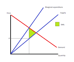
The excess capacity theorem assumes a classical production function and corresponding cost curves as well as the same costs for all producers. Figure 6.4 illustrates the situation. The demand curve is again downward sloping and the slope of marginal revenue curve is twice as much as the demand curve. The marginal cost curve (supply) is upward sloping. As there are some fixed costs, total average costs are U-shaped. Profit maximizing is the quantity $q^{m c}$ where marginal costs equal marginal revenue and the corresponding price is $p^{m c}$. If the average total cost curve lies below the demand curve, the monopolistic competitor generates a profit.
The strength of consumer preferences for a differentiated product is represented in the elasticity of the demand curve. The stronger the preference, the more inelastic will be the demand curve (Figure 6.4, right).
In the short run, the monopolistic competitor will act as monopolist dealing with cost curves from the classical production function (Figure 6.5, left). With market entry, the demand and marginal revenue curves will swivel around point $\mathrm{A}$ and become more elastic. The $y$-intercept moves from B to B’ (Figure 6.5, right). The price is lowered and the offered quantity is also reduced. This reduces the monopolistic profit.
经济代写|微观经济学代写Microeconomics代考|Monopsony
Monopsonies play a role in the construction sector. The government or government agencies act sometimes as the sole buyer in a market. In many countries, it is the exclusive right and duty of the government to provide public roads. As these are by far the majority of all roads, the government acts as monopsonist. The same often holds true for railroads. Thus, monopsonies are of interest. The owner in construction will not be a consumer (one-family home) but an investor and will thus act on factor markets (Chapter 7).
A typical case in the microeconomic literature to explain monopsonies is one employer looking for labor (Nicholson and Snyder 2014). This could be a large firm in a small town. If one producer is the asking for the by-far-largest supply of labor from a relatively large number of workers, then that producer holds a monopsony position. This is the inverse of a monopoly.
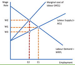
If we call $p \cdot \partial q / \partial L$ the marginal value product of labor $\left(M V P_L\right)$, then we know that this must equal the wage if the producer is maximizing the profit in perfectly competitive markets. If we assume diminishing marginal labor productivity, then the $\mathrm{MVP}_{\mathrm{L}}$ curve is downward sloping (Figure 6.8).
The labor supply curve is sloping upward because the monopsonist is not facing a negligible quantity of labor but the majority of the labor supply in a regional market. If the monpsonist hires one more worker, this worker is only willing to accept above market price. If all workers receive the same wage, this means that adding one more worker increases total cost by the pay for the worker and the increase for all other workers. The cost of hiring one more worker is always higher than the market price. Consequently, the marginal expense curve will always be above the labor supply curve.
A producer in a perfectly competitive market will hire more labor until the additional marginal costs $M E_{\mathrm{L}}$ are equal to the additional marginal revenue $M R_{\mathrm{L}}$. If the costs were higher, then the producer would lose money; if the costs were lower, it would forgo the opportunity to increase its profit:
$$
M E_{\mathrm{L}}=M R_{\mathrm{L}}
$$
The monopsonist will add labor until the marginal revenue of labor equals the MVP:
$$
M R_{\mathrm{L}}=M V P_{\mathrm{L}}
$$
If the producer were a price taker, then the intersection of the downward-sloping demand curve and the upward-sloping supply curve would provide the market equilibrium. This is marked as $L_{\mathrm{C}}$ and $w_{\mathrm{C}}$ in Figure 6.9. Since a monopsonist is not a price taker, the marginal revenue curve (expense curve) lies above the supply curve and this determines actual labor demand by $M R_{\mathrm{L}}=M V P_{\mathrm{L}}$. Thus, the monopsonist demands less labor $\left(L_{\mathrm{M}}\right)$ at a lower wage $\left(w_M\right)$ by using its market power.
The more inelastic the labor supply curve is, the lower will the wage be. To see this effect, you just have to rotate the supply curve more upward around the point $L_{\mathrm{C}} / w_{\mathrm{C}}$.
微观经济学代考
经济代写|微观经济学代写Microeconomics代考|Monopolistic Competition
垄断竞争是除异质寡头垄断之外最普遍的市场配置。在这些条件下,生产商提供差异化产品——而不是同质产品——服务于相同的目的,例如 T 恤,消费者对某些产品有偏好。这为生产商设定价格提供了一些空间。他们不再是价格接受者,但他们也没有正常垄断者的自由。他们的市场力量更加有限。生产商可以主要通过风格、位置或质量来区分产品。生产者越能够区分产品,市场力量就越强。每个生产者只向市场提供相对少量的商品,因此其行为不会影响其他生产者。因此,如果生产者提高产品价格,
然而,生产者受到可以进入市场并攻击差异化产品的新公司的威胁。从长远来看,自由市场进入的可能性会使利润减少到零。这个结果与完全竞争相同,但其他结果不同,我们将看到。
产能过剩定理假设一个经典的生产函数和相应的成本曲线以及所有生产者的相同成本。图 6.4 说明了这种情况。需求曲线再次向下倾斜,边际收益曲线的斜率是需求曲线的两倍。边际成本曲线(供给)向上倾斜。由于有一些固定成本,总平均成本呈 U 形。利润最大化是数量q米C其中边际成本等于边际收益,相应的价格是p米C. 如果平均总成本曲线位于需求曲线下方,则垄断竞争者产生利润。
消费者对差异化产品的偏好强度体现在需求曲线的弹性上。偏好越强,需求曲线就越缺乏弹性(图 6.4,右)。
在短期内,垄断竞争者将作为垄断者处理经典生产函数的成本曲线(图 6.5,左)。随着市场进入,需求和边际收益曲线将围绕点旋转A并变得更有弹性。这和-拦截从 B 移动到 B’(图 6.5,右)。价格降低,报价数量也减少。这减少了垄断利润。
经济代写|微观经济学代写Microeconomics代考|Monopsony
垄断在建筑行业发挥作用。政府或政府机构有时充当市场上的唯一买家。在许多国家,提供公共道路是政 府的专有权利和义务。由于这些是迄今为止所有道路中的大多数,因此政府充当垄断者。铁路也是如此。 因此,芢断是令人感兴趣的。建筑业主将不是消费者(单户住宅),而是投资者,因此将在要素市场上行 动(第 7 章)。
微观经济学文献中解释垄断的典型案例是一个雇主在寻找劳动力 (Nicholson 和 Snyder 2014)。这可能 是一个小镇上的大公司。如果一个生产者要求相对大量的工人提供迄今为止最大的劳动力供应,那么该生 产者就处于垄断地位。这与䞣断相反。
如果我们打电话 $p \cdot \partial q / \partial L$ 劳动的边际价值产品 $\left(M V P_L\right)$ ,那么我们就知道,如果生产者在完全竞争市场 上实现利润最大化,那么这一定等于工资。如果我们假设边际劳动生产率递减,那么 $M_V \mathrm{PP}{\mathrm{L}}$ 曲线向下倾斜 (图 6.8)。 劳动力供给曲线向上倾斜,因为龿断者面对的不是微不足道的劳动力,而是区域市场中的大部分劳动力供 给。如果 monpsonist 再雇用一名工人,这名工人只愿意接受高于市场价格的价格。如果所有工人获得相 司的工资,这意味着增加一名工人会增加总成本,增加的部分是该工人的工资和所有其他工人的增加。多 蒮一名工人的成本总是高于市场价格。因此,边际费用曲线将始终高于劳动力供给曲线。 完全竞争市场中的生产者将雇佣更多的劳动力,直到额外的边际成本 $M E{\mathrm{L}}$ 等于额外的边际收益 $M R_{\mathrm{L}}$. 如 果成本更高,那么生产商就会赔钱;如果成本较低,它将放弃增加利润的机会:
$$
M E_{\mathrm{L}}=M R_{\mathrm{L}}
$$
垄断者将增加劳动力,直到劳动力的边际收益等于 MVP:
$$
M R_{\mathrm{L}}=M V P_{\mathrm{L}}
$$
如果生产者是价格接受者,那么向下倾斜的需求曲线和向上倾斜的供给曲线的交点将提供市场均衡。这被 标记为 $L_{\mathrm{C}}$ 和 $w_{\mathrm{C}}$ 在图 6.9 中。由于垄断者不是价格接受者,边际收益曲线 (费用曲线) 位于供给曲线之 上,这决定了实际劳动力需求 $M R_{\mathrm{L}}=M V P_{\mathrm{L}}$. 因此,垄断者需要更少的劳动力 $\left(L_{\mathrm{M}}\right)$ 以较低的工资 $\left(w_M\right)$ 通过利用其市场力量。
劳动力供给曲线越缺乏弹性,工资就越低。要看到这种效果,您只需将供应曲线围绕该点向上旋转
$$
L_{\mathrm{C}} / w_{\mathrm{C}}
$$

统计代写请认准statistics-lab™. statistics-lab™为您的留学生涯保驾护航。
金融工程代写
金融工程是使用数学技术来解决金融问题。金融工程使用计算机科学、统计学、经济学和应用数学领域的工具和知识来解决当前的金融问题,以及设计新的和创新的金融产品。
非参数统计代写
非参数统计指的是一种统计方法,其中不假设数据来自于由少数参数决定的规定模型;这种模型的例子包括正态分布模型和线性回归模型。
广义线性模型代考
广义线性模型(GLM)归属统计学领域,是一种应用灵活的线性回归模型。该模型允许因变量的偏差分布有除了正态分布之外的其它分布。
术语 广义线性模型(GLM)通常是指给定连续和/或分类预测因素的连续响应变量的常规线性回归模型。它包括多元线性回归,以及方差分析和方差分析(仅含固定效应)。
有限元方法代写
有限元方法(FEM)是一种流行的方法,用于数值解决工程和数学建模中出现的微分方程。典型的问题领域包括结构分析、传热、流体流动、质量运输和电磁势等传统领域。
有限元是一种通用的数值方法,用于解决两个或三个空间变量的偏微分方程(即一些边界值问题)。为了解决一个问题,有限元将一个大系统细分为更小、更简单的部分,称为有限元。这是通过在空间维度上的特定空间离散化来实现的,它是通过构建对象的网格来实现的:用于求解的数值域,它有有限数量的点。边界值问题的有限元方法表述最终导致一个代数方程组。该方法在域上对未知函数进行逼近。[1] 然后将模拟这些有限元的简单方程组合成一个更大的方程系统,以模拟整个问题。然后,有限元通过变化微积分使相关的误差函数最小化来逼近一个解决方案。
tatistics-lab作为专业的留学生服务机构,多年来已为美国、英国、加拿大、澳洲等留学热门地的学生提供专业的学术服务,包括但不限于Essay代写,Assignment代写,Dissertation代写,Report代写,小组作业代写,Proposal代写,Paper代写,Presentation代写,计算机作业代写,论文修改和润色,网课代做,exam代考等等。写作范围涵盖高中,本科,研究生等海外留学全阶段,辐射金融,经济学,会计学,审计学,管理学等全球99%专业科目。写作团队既有专业英语母语作者,也有海外名校硕博留学生,每位写作老师都拥有过硬的语言能力,专业的学科背景和学术写作经验。我们承诺100%原创,100%专业,100%准时,100%满意。
随机分析代写
随机微积分是数学的一个分支,对随机过程进行操作。它允许为随机过程的积分定义一个关于随机过程的一致的积分理论。这个领域是由日本数学家伊藤清在第二次世界大战期间创建并开始的。
时间序列分析代写
随机过程,是依赖于参数的一组随机变量的全体,参数通常是时间。 随机变量是随机现象的数量表现,其时间序列是一组按照时间发生先后顺序进行排列的数据点序列。通常一组时间序列的时间间隔为一恒定值(如1秒,5分钟,12小时,7天,1年),因此时间序列可以作为离散时间数据进行分析处理。研究时间序列数据的意义在于现实中,往往需要研究某个事物其随时间发展变化的规律。这就需要通过研究该事物过去发展的历史记录,以得到其自身发展的规律。
回归分析代写
多元回归分析渐进(Multiple Regression Analysis Asymptotics)属于计量经济学领域,主要是一种数学上的统计分析方法,可以分析复杂情况下各影响因素的数学关系,在自然科学、社会和经济学等多个领域内应用广泛。
MATLAB代写
MATLAB 是一种用于技术计算的高性能语言。它将计算、可视化和编程集成在一个易于使用的环境中,其中问题和解决方案以熟悉的数学符号表示。典型用途包括:数学和计算算法开发建模、仿真和原型制作数据分析、探索和可视化科学和工程图形应用程序开发,包括图形用户界面构建MATLAB 是一个交互式系统,其基本数据元素是一个不需要维度的数组。这使您可以解决许多技术计算问题,尤其是那些具有矩阵和向量公式的问题,而只需用 C 或 Fortran 等标量非交互式语言编写程序所需的时间的一小部分。MATLAB 名称代表矩阵实验室。MATLAB 最初的编写目的是提供对由 LINPACK 和 EISPACK 项目开发的矩阵软件的轻松访问,这两个项目共同代表了矩阵计算软件的最新技术。MATLAB 经过多年的发展,得到了许多用户的投入。在大学环境中,它是数学、工程和科学入门和高级课程的标准教学工具。在工业领域,MATLAB 是高效研究、开发和分析的首选工具。MATLAB 具有一系列称为工具箱的特定于应用程序的解决方案。对于大多数 MATLAB 用户来说非常重要,工具箱允许您学习和应用专业技术。工具箱是 MATLAB 函数(M 文件)的综合集合,可扩展 MATLAB 环境以解决特定类别的问题。可用工具箱的领域包括信号处理、控制系统、神经网络、模糊逻辑、小波、仿真等。