如果你也在 怎样代写多元统计分析Multivariate Statistical Analysis这个学科遇到相关的难题,请随时右上角联系我们的24/7代写客服。
多变量统计分析被认为是评估地球化学异常与任何单独变量和变量之间相互影响的意义的有用工具。
statistics-lab™ 为您的留学生涯保驾护航 在代写多元统计分析Multivariate Statistical Analysis方面已经树立了自己的口碑, 保证靠谱, 高质且原创的统计Statistics代写服务。我们的专家在代写多元统计分析Multivariate Statistical Analysis代写方面经验极为丰富,各种代写多元统计分析Multivariate Statistical Analysis相关的作业也就用不着说。
我们提供的多元统计分析Multivariate Statistical Analysis及其相关学科的代写,服务范围广, 其中包括但不限于:
- Statistical Inference 统计推断
- Statistical Computing 统计计算
- Advanced Probability Theory 高等概率论
- Advanced Mathematical Statistics 高等数理统计学
- (Generalized) Linear Models 广义线性模型
- Statistical Machine Learning 统计机器学习
- Longitudinal Data Analysis 纵向数据分析
- Foundations of Data Science 数据科学基础
统计代写|多元统计分析代写Multivariate Statistical Analysis代考|Lasso in the Linear Regression Model
The linear regression model can be written as follows:
$$
y=\mathcal{X} \beta+\varepsilon,
$$
where $y$ is an $(n \times 1)$ vector of observations for the response variable, $\mathcal{X}=$ $\left(x_1^{\top}, \ldots, x_n^{\top}\right)^{\top}, x_i \in \mathbb{R}^p, i=1, \ldots, n$ is a data matrix of $p$ explanatory variables, and $\varepsilon=\left(\varepsilon_1, \ldots, \varepsilon_n\right)^{\top}$ is a vector of errors where $\mathrm{E}\left(\varepsilon_i\right)=0$ and $\operatorname{Var}\left(\varepsilon_i\right)=\sigma^2$, $i=1, \ldots, n$.
In this framework, $\mathrm{E}(y \mid \mathcal{X})=\mathcal{X} \beta$ with $\beta=\left(\beta_1, \ldots, \beta_p\right)^{\top}$. Further assume that the columns of $\mathcal{X}$ are standardised such that $n^{-1} \sum_{i=1}^n x_{i j}=0$ and $n^{-1} \sum_{i=1}^n x_{i j}^2=$ 1. The Lasso estimate $\hat{\beta}$ can then be defined as follows
$$
\hat{\beta}=\arg \min \beta\left{\sum{i=1}^n\left(y_i-x_i^{\top} \beta\right)^2\right}, \text { subject to } \sum_{j=1}^p\left|\beta_j\right| \leq s,
$$
where $s \geq 0$ is the tuning parameter which controls the amount of shrinkage. For the OLS estimate $\hat{\beta}^0=\left(\mathcal{X}^{\top} \mathcal{X}\right)^{-1} \mathcal{X}^{\top} y$ a choice of tuning parameter $s<s_0$, where $s_0=\sum_{j=1}^p\left|\hat{\beta}j^0\right|$, will cause shrinkage of the solutions towards 0 , and ultimately some coefficients may be exactly equal to 0 . For values $s \geq s_0$ the Lasso coefficients are equal to the unpenalised OLS coefficients. An alternative representation of $(9.1)$ is: $$ \hat{\beta}=\arg \min \beta\left{\sum_{i=1}^n\left(y_i-x_i^{\top} \beta\right)^2+\lambda \sum_{j=1}^p\left|\beta_j\right|\right},
$$ with a tuning parameter $\lambda \geq 0$. As $\lambda$ increases, the Lasso estimates are continuously shrunk toward zero. Then if $\lambda$ is quite large, some coefficients are exactly zero. For $\lambda=0$ the Lasso coefficients coincide with the OLS estimate. In fact, if the solution to (9.1) is denoted as $\hat{\beta}s$ and the solution to (9.2) as $\hat{\beta}\lambda$, then $\forall \lambda>0$ and the resulting solution $\hat{\beta}\lambda \exists s\lambda$ such that $\hat{\beta}\lambda=\hat{\beta}{s_\lambda}$ and vice versa which implies a one-toone correspondence between these parameters. However, this does not hold if it is required that $\lambda \geq 0$ only and not $\lambda>0$, because if, for instance, $\lambda=0$, then $\hat{\beta}_\lambda$ is the same for any $s \geq|\hat{\beta}|_1$ and the correspondence is no longer one-to-one.
统计代写|多元统计分析代写Multivariate Statistical Analysis代考|The LAR Algorithm and Lasso Solution Paths
The LAR algorithm may be introduced in the simple three-dimensional case as follows (assume that the number of covariates $p=3$ ):
- first, standardise all the covariates to have mean 0 and unit length as well as make the response variable have mean zero;
- start with $\hat{\beta}=0$;
- initialise the algorithm with the first two covariates: let $\mathcal{X}=\left(x_1, x_2\right)$ and calculate the prediction vector $\hat{y}_0=\mathcal{X} \hat{\beta}=0$;
- calculate $\bar{y}_2$ the projection of $y$ onto $\mathcal{L}\left(x_1, x_2\right)$, the linear space spanned by $x_1$ and $x_2$
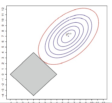
- compute the vector of current correlations between the covariates $\mathcal{X}$ and the two-dimensional current residual vector: $C^{\hat{y}_0}=\mathcal{X}^{\top}\left(\bar{y}_2-\hat{y}_0\right)=\left(c_1^{\hat{y}_0}, c_2^{\hat{y}_0}\right)^{\top}$. According to Fig.9.2, the current residual $\bar{y}_2-\hat{y}_0$ makes a smaller angle with $x_1$, than with $x_2$, therefore $c_1^{\hat{y}}>c_2^{\hat{y_0}}$;
- augment $\hat{y}_0$ in the direction of $x_1$ so that $\hat{y}_1=\hat{y}_0+\hat{\gamma}_1 x_1$ with $\hat{\gamma}_1$ chosen such that $c_1^{\hat{y}_0}=c_2^{\hat{y}_0}$ which means that the new current residual $\bar{y}_2-\hat{y}_1$ makes equal angles (is equiangular) with $x_1$ and $x_2$;
- suppose that another regressor $x_3$ enters the model: calculate a new projection $\bar{y}_3$ of $y$ onto $\mathcal{L}\left(x_1, x_2, x_3\right)$;
- recompute the current correlations vector $C^{\hat{y}_1}=\left(c_1^{\hat{y}_1}, c_2^{\hat{y}_1}, c_3^{\hat{y}_1}\right)^{\top}$ with $\mathcal{X}=$ $\left(x_1, x_2, x_3\right), \bar{y}_3$ and $\hat{y}_1$;
- augment $\hat{y}_1$ in the equiangular direction so that $\hat{y}_2=\hat{y}_1+\hat{\gamma}_2 u_2$ with $\hat{\gamma}_2$ chosen such that $c_1^{\hat{y_1}}=c_2^{\hat{y_1}}=c_3^{\hat{y_1}}$, then the new current residual $\bar{y}_3-\hat{y}_2$ goes
- equiangularly between $x_1, x_2$ and $x_3$ (here $u_2$ is the unit vector lying along the equiangular direction $\hat{y}_2$ );
- the three-dimensional algorithm is terminated with the calculation of the final prediction vector $\hat{y}_3=\hat{y}_2+\hat{\gamma}_3 u_3$ with $\hat{\gamma}_3$ chosen such that $\hat{y}_3=\bar{y}_3$.
- In the case of $p>3$ covariates, $\hat{y}_3$ would be smaller than $\bar{y}_3$ initiating another change of direction, as illustrated in Fig. 9.2.
- In this setup, it is important that the covariate vectors $x_1, x_2, x_3$ are linearly independent. The LAR algorithm “moves” the variable coefficients to their least squares values. So the Lasso adjustment necessary for the sparse solution is that if a nonzero coefficient happens to return to zero, it should be dropped from the current (“active”) set of variables and not be considered in further computations. The general LAR algorithm for $p$ predictors can be summarised as follows.
多元统计分析代考
统计代写|多元统计分析代写Multivariate Statistical Analysis代考|Lasso in the Linear Regression Model
线性回归模型可以写成如下:
$$
y=\mathcal{X} \beta+\varepsilon,
$$
在哪里 $y$ 是一个 $(n \times 1)$ 响应变量的观察向量, $\mathcal{X}=\left(x_1^{\top}, \ldots, x_n^{\top}\right)^{\top}, x_i \in \mathbb{R}^p, i=1, \ldots, n$ 是一个数 据矩阵 $p$ 解释变量,和 $\varepsilon=\left(\varepsilon_1, \ldots, \varepsilon_n\right)^{\top}$ 是错误向量,其中 $\mathrm{E}\left(\varepsilon_i\right)=0$ 和 $\operatorname{Var}\left(\varepsilon_i\right)=\sigma^2$ , $i=1, \ldots, n$
在这个框架下, $\mathrm{E}(y \mid \mathcal{X})=\mathcal{X} \beta$ 和 $\beta=\left(\beta_1, \ldots, \beta_p\right)^{\top}$. 进一步假设列 $\mathcal{X}$ 被标准化使得 $n^{-1} \sum_{i=1}^n x_{i j}=0$ 和 $n^{-1} \sum_{i=1}^n x_{i j}^2=1$. Lasso估计 $\hat{\beta}$ 然后可以定义如下
在哪里 $s \geq 0$ 是控制收缩量的调整参数。对于 OLS 估计 $\hat{\beta}^0=\left(\mathcal{X}^{\top} \mathcal{X}\right)^{-1} \mathcal{X}^{\top} y$ 调整参数的选择 $s0$ 以及由此产生的解决方案 $\hat{\beta} \lambda \exists s \lambda$ 这样 $\hat{\beta} \lambda=\hat{\beta} s_\lambda$ 反之亦然,这意味着这些参数之间存在一对一的 对应关系。但是,如果要求 $\lambda \geq 0$ 只有而不是 $\lambda>0$ ,因为如果,例如, $\lambda=0$ ,然后 $\hat{\beta}_\lambda$ 对任何一个都 是一样的 $s \geq|\hat{\beta}|_1$ 并且对应关系不再是一对一的。
统计代写|多元统计分析代写Multivariate Statistical Analysis代考|The LAR Algorithm and Lasso Solution Paths
LAR算法可以在简单的三维情况下引入如下 (假设协变量的数量 $p=3$ ):
- 首先,将所有协变量标准化为均值为 0 和单位长度,并使响应变量的均值为零;
- 从…开始 $\hat{\beta}=0$;
- 用前两个协变量初始化算法: 让 $\mathcal{X}=\left(x_1, x_2\right)$ 并计算预测向量 $\hat{y}_0=\mathcal{X} \hat{\beta}=0$;
- 计算 $\bar{y}_2$ 的投射 $y$ 到 $\mathcal{L}\left(x_1, x_2\right)$ ,线性空间跨越 $x_1$ 和 $x_2$
- 计算协变量之间当前相关性的向量 $\mathcal{X}$ 和二维当前残差向量:
$C^{\hat{y}_0}=\mathcal{X}^{\top}\left(\bar{y}_2-\hat{y}_0\right)=\left(c_1^{\hat{y}_0}, c_2^{\hat{y}_0}\right)^{\top}$. 根据图 9.2,当前残差 $\bar{y}_2-\hat{y}_0$ 与 $x_1$ ,比与 $x_2$ ,所以 $c_1^{\hat{y}}>c_2^{\hat{y_0}}$; - 增加 $\hat{y}_0$ 在…方向 $x_1$ 以便 $\hat{y}_1=\hat{y}_0+\hat{\gamma}_1 x_1$ 和 $\hat{\gamma}_1$ 选择这样的 $c_1^{\hat{y}_0}=c_2^{\hat{y}_0}$ 这意味着新的当前残差 $\bar{y}_2-\hat{y}_1$ 使角相等 (等角) 与 $x_1$ 和 $x_2$ ;
- 假设另一个回归量 $x_3$ 进入模型: 计算一个新的投影 $\bar{y}_3$ 的 $y$ 到 $\mathcal{L}\left(x_1, x_2, x_3\right)$;
- 重新计算当前相关向量 $C^{\hat{y}_1}=\left(c_1^{\hat{y}_1}, c_2^{\hat{y}_1}, c_3^{\hat{y}_1}\right)^{\top}$ 和 $\mathcal{X}=\left(x_1, x_2, x_3\right), \bar{y}_3$ 和 $\hat{y}_1$ ;
- 增加 $\hat{y}_1$ 在等角方向,使得 $\hat{y}_2=\hat{y}_1+\hat{\gamma}_2 u_2$ 和 $\hat{\gamma}_2$ 选择这样的 $c_1^{\hat{y}_1}=c_2^{\hat{y_1}}=c_3^{\hat{y_1}}$ ,那么新的当前残差 $\bar{y}_3-\hat{y}_2$ 去
- 之间等角 $x_1, x_2$ 和 $x_3$ (这里 $u_2$ 是沿等角方向的单位向量 $\hat{y}_2$ );
- 三维算法以最终预测向量的计算结束 $\hat{y}_3=\hat{y}_2+\hat{\gamma}_3 u_3$ 和 $\hat{\gamma}_3$ 选择这样的 $\hat{y}_3=\bar{y}_3$.
- 如果是 $p>3$ 协变量, $\hat{y}_3$ 会小于 $\bar{y}_3$ 开始另一个方向改变,如图 $9.2$ 所示。
- 在此设置中,重要的是协变量向量 $x_1, x_2, x_3$ 是线性独立的。LAR 算法将可变系数“移动”到它们的最 小二乘值。因此,稀疏解决方案所需的套索调整是,如果非零系数恰好返回零,则应将其从当前
(“活动”) 变量集中删除,并且在进一步的计算中不予考虑。一般的 LAR 算法为 $p$ 预测因素可以总结 如下。

统计代写请认准statistics-lab™. statistics-lab™为您的留学生涯保驾护航。
金融工程代写
金融工程是使用数学技术来解决金融问题。金融工程使用计算机科学、统计学、经济学和应用数学领域的工具和知识来解决当前的金融问题,以及设计新的和创新的金融产品。
非参数统计代写
非参数统计指的是一种统计方法,其中不假设数据来自于由少数参数决定的规定模型;这种模型的例子包括正态分布模型和线性回归模型。
广义线性模型代考
广义线性模型(GLM)归属统计学领域,是一种应用灵活的线性回归模型。该模型允许因变量的偏差分布有除了正态分布之外的其它分布。
术语 广义线性模型(GLM)通常是指给定连续和/或分类预测因素的连续响应变量的常规线性回归模型。它包括多元线性回归,以及方差分析和方差分析(仅含固定效应)。
有限元方法代写
有限元方法(FEM)是一种流行的方法,用于数值解决工程和数学建模中出现的微分方程。典型的问题领域包括结构分析、传热、流体流动、质量运输和电磁势等传统领域。
有限元是一种通用的数值方法,用于解决两个或三个空间变量的偏微分方程(即一些边界值问题)。为了解决一个问题,有限元将一个大系统细分为更小、更简单的部分,称为有限元。这是通过在空间维度上的特定空间离散化来实现的,它是通过构建对象的网格来实现的:用于求解的数值域,它有有限数量的点。边界值问题的有限元方法表述最终导致一个代数方程组。该方法在域上对未知函数进行逼近。[1] 然后将模拟这些有限元的简单方程组合成一个更大的方程系统,以模拟整个问题。然后,有限元通过变化微积分使相关的误差函数最小化来逼近一个解决方案。
tatistics-lab作为专业的留学生服务机构,多年来已为美国、英国、加拿大、澳洲等留学热门地的学生提供专业的学术服务,包括但不限于Essay代写,Assignment代写,Dissertation代写,Report代写,小组作业代写,Proposal代写,Paper代写,Presentation代写,计算机作业代写,论文修改和润色,网课代做,exam代考等等。写作范围涵盖高中,本科,研究生等海外留学全阶段,辐射金融,经济学,会计学,审计学,管理学等全球99%专业科目。写作团队既有专业英语母语作者,也有海外名校硕博留学生,每位写作老师都拥有过硬的语言能力,专业的学科背景和学术写作经验。我们承诺100%原创,100%专业,100%准时,100%满意。
随机分析代写
随机微积分是数学的一个分支,对随机过程进行操作。它允许为随机过程的积分定义一个关于随机过程的一致的积分理论。这个领域是由日本数学家伊藤清在第二次世界大战期间创建并开始的。
时间序列分析代写
随机过程,是依赖于参数的一组随机变量的全体,参数通常是时间。 随机变量是随机现象的数量表现,其时间序列是一组按照时间发生先后顺序进行排列的数据点序列。通常一组时间序列的时间间隔为一恒定值(如1秒,5分钟,12小时,7天,1年),因此时间序列可以作为离散时间数据进行分析处理。研究时间序列数据的意义在于现实中,往往需要研究某个事物其随时间发展变化的规律。这就需要通过研究该事物过去发展的历史记录,以得到其自身发展的规律。
回归分析代写
多元回归分析渐进(Multiple Regression Analysis Asymptotics)属于计量经济学领域,主要是一种数学上的统计分析方法,可以分析复杂情况下各影响因素的数学关系,在自然科学、社会和经济学等多个领域内应用广泛。
MATLAB代写
MATLAB 是一种用于技术计算的高性能语言。它将计算、可视化和编程集成在一个易于使用的环境中,其中问题和解决方案以熟悉的数学符号表示。典型用途包括:数学和计算算法开发建模、仿真和原型制作数据分析、探索和可视化科学和工程图形应用程序开发,包括图形用户界面构建MATLAB 是一个交互式系统,其基本数据元素是一个不需要维度的数组。这使您可以解决许多技术计算问题,尤其是那些具有矩阵和向量公式的问题,而只需用 C 或 Fortran 等标量非交互式语言编写程序所需的时间的一小部分。MATLAB 名称代表矩阵实验室。MATLAB 最初的编写目的是提供对由 LINPACK 和 EISPACK 项目开发的矩阵软件的轻松访问,这两个项目共同代表了矩阵计算软件的最新技术。MATLAB 经过多年的发展,得到了许多用户的投入。在大学环境中,它是数学、工程和科学入门和高级课程的标准教学工具。在工业领域,MATLAB 是高效研究、开发和分析的首选工具。MATLAB 具有一系列称为工具箱的特定于应用程序的解决方案。对于大多数 MATLAB 用户来说非常重要,工具箱允许您学习和应用专业技术。工具箱是 MATLAB 函数(M 文件)的综合集合,可扩展 MATLAB 环境以解决特定类别的问题。可用工具箱的领域包括信号处理、控制系统、神经网络、模糊逻辑、小波、仿真等。