如果你也在 怎样代写数值分析numerical analysis这个学科遇到相关的难题,请随时右上角联系我们的24/7代写客服。
数值分析是数学的一个分支,使用数字近似法解决连续问题。它涉及到设计能给出近似但精确的数字解决方案的方法,这在精确解决方案不可能或计算成本过高的情况下很有用。
statistics-lab™ 为您的留学生涯保驾护航 在代写数值分析numerical analysis方面已经树立了自己的口碑, 保证靠谱, 高质且原创的统计Statistics代写服务。我们的专家在代写数值分析numerical analysis代写方面经验极为丰富,各种代写数值分析numerical analysis相关的作业也就用不着说。
我们提供的数值分析numerical analysis及其相关学科的代写,服务范围广, 其中包括但不限于:
- Statistical Inference 统计推断
- Statistical Computing 统计计算
- Advanced Probability Theory 高等概率论
- Advanced Mathematical Statistics 高等数理统计学
- (Generalized) Linear Models 广义线性模型
- Statistical Machine Learning 统计机器学习
- Longitudinal Data Analysis 纵向数据分析
- Foundations of Data Science 数据科学基础

数学代写|数值分析代写numerical analysis代考|NONLINEAR EQUATIONS
The first method we will consider is the method of exhaustive search (also called direct, graphical, or incremental search). Suppose that $f$ is continuous on some (not necessarily finite) interval. By the Intermediate Value Theorem, if we can find two points $a, b$ such that $f(a)$ and $f(b)$ have opposite signs, then a zero of $f$ must lie in $(a, b)$. One way to find such a pair of points is to pick some number $x_0$ as an initial guess as to the location of a root and successively evaluate the function at
$$
x_0, x_1=x_0+h, x_2=x_0+2 h, x_3=x_0+3 h, \ldots
$$
where $h>0$ is called the step size (or grid size). When a change of sign is detected, we say that we have bracketed a root in this interval of width $h$. (The interval $\left[x_i, x_{i+1}\right]$ over which the change of sign occurs is called a bracket; see Fig. 1, where the endpoints form a bracket.) At this point we may repeat the process over the smaller interval $\left[x_i, x_{i+1}\right]$ with a smaller $h$ in order to bracket the root more precisely.
The exhaustive search method is equivalent to plotting the function and looking for an interval in which it crosses the $x$-axis. This is very inefficient, so let’s look for a better approach. Suppose that we have found a bracket $[a, b]$ for a zero of a continuous function (by any means). Rather than searching the entire interval with a finer step size, we might reason that the midpoint
$$
m=\frac{a+b}{2}
$$
is a better estimate of the location of the true zero $x^$ of $f$ than either $a$ or $b$; after all, $\left|a-x^\right|$ could be as large as the width $w=(b-a)$ of the interval if $x^$ is near $b$, and similarly for $\left|b-x^\right|$, but
$$
\left|m-x^\right| \leq \frac{1}{2} w $$ since $x^$ lies either in the interval to the right or to the left of $m$ (or both, in the extremely unlikely case that $x^*=m$ ). This is the idea behind the bisection method (or binary search): If $f$ is continuous on some interval and $\left[x_0, x_1\right]$ is a bracket, that is, if $f\left(x_0\right) f\left(x_1\right)<0$, then we set $$
x_2=\frac{x_0+x_1}{2}
$$
and compute $f\left(x_2\right)$. If $f\left(x_2\right)=0$, we are done; otherwise either $f\left(x_2\right)$ and $f\left(x_0\right)$ have opposite signs, in which case $\left[x_0, x_2\right]$ is a new bracket half the size of the previous one, or $f\left(x_2\right)$ and $f\left(x_1\right)$ have opposite signs, in which case $\left[x_2, x_1\right]$ is a new bracket half the size of the previous one. In either case we have reduced our uncertainty as to the location of the true zero $x^*$ by $50 \%$ at the cost of a single new function evaluation (namely the computation of $f\left(x_2\right)$ ). We may now repeat this process on the new interval, finding its midpoint $x_3$ and then a smaller bracket with $x_3$ as an endpoint, and so on, until a sufficiently narrow bracket is obtained.
数学代写|数值分析代写numerical analysis代考|BISECTION AND INVERSE LINEAR INTERPOLATION
which is a pretty good point estimate of $\pi / 2=1.57079 \ldots$, and as $\cos (1.5649)=$ $5.8963 \times 10^{-3}$ is positive it leads to the new bracket $[1.5649,2]$ which is slightly smaller than the bracket $[1.5,2]$ found by bisection after one step. The next step gives
$$
\begin{aligned}
x_3 & =x_2-f\left(x_2\right) \frac{x_2-x_1}{f\left(x_2\right)-f\left(x_1\right)} \
& =1.5649-\cos (1.5649) \frac{1.5649-2}{\cos (1.5649)-\cos (2)} \
& \doteq 1.5710
\end{aligned}
$$
(where we would be re-using the previously computed cosine values rather than re-computing them.) Since $\cos (1.5710)<0$, the new bracket is $[1.5649,1.5710]$. Its width is $1.5710-1.5649=0.0061$, a vast improvement over the corresponding width of $.25$ for bisection, and the midpoint of this interval is an excellent estimate of the root.
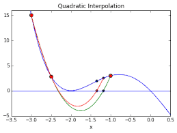
Inverse linear interpolation will converge to some zero of the function in the bracket; however, the rate at which it converges will depend on how nearly linear $f(x)$ is near its zero. If $f(x)$ is well approximated by a straight line over the bracket, the method will usually be faster than bisection. (A function and bracket as in Fig. 4 will result in excruciatingly slow convergence until the bracket is very small.) We have given up the guaranteed slow-but-steady-wins-the-race speed of bisection for a likely but neither guaranteed nor easily predictable improvement.
In the next section we will consider a much faster algorithm known as Newton’s method. Once again a price will be paid: We will require that the function be differentiable as well. Faster methods will require more assumptions and will offer fewer guarantees. But first: MATLAB ${ }^{(\mathrm{R}}$.
数值分析代考
数学代写|数值分析代写numerical analysis代考|NONLINEAR EQUATIONS
我们要考虑的第一种方法是穷举搜索法 (也称为直接搜索、图形搜索或增量搜索) 。假设 $f$ 在某个 (不 一定是有限的) 区间上是连续的。根据中值定理,如果我们能找到两点 $a, b$ 这样 $f(a)$ 和 $f(b)$ 有相反的 符号,然后是零 $f$ 必须躬在 $(a, b)$. 找到这样一对点的一种方法是选择一些数字 $x_0$ 作为对根位置的初始 猜测,并连续评估函数
$$
x_0, x_1=x_0+h, x_2=x_0+2 h, x_3=x_0+3 h, \ldots
$$
在哪里 $h>0$ 称为步长 (或网格大小) 。当检测到符号变化时,我们说我们在这个宽度区间内包含了一 个根 $h$. (间隔 $\left.x_i, x_{i+1}\right]$ 发生符号变化的括号称为括号;参见图 1,其中端点形成一个括号。) 此时我 们可以在较小的间隔内重复该过程 $\left[x_i, x_{i+1}\right]$ 用更小的 $h$ 为了更精确地括起根。
穷举搜索法相当于绘制函数并寻找它与 $x$-轴。这是非常低效的,所以让我们寻找更好的方法。假设我 们找到了一个括号 $[a, b]$ 对于连续函数的零 (无论如何) 。与其以更精细的步长搜索整个区间,我们可 能会推断中点
$$
m=\frac{a+b}{2}
$$
是对真零位置的更好估计 $\mathrm{x}^{\wedge}$ 的 $f$ 比任何一个 $a$ 或者 $b$; 毕竟,左|轴^右|可能和宽度一样大 $w=(b-a)$ 区间的如果 $\mathrm{x}^{\wedge}$ 近 $b$, 同样对于 $\left|b^2\right| \mathrm{bx} \mathrm{x}^{\wedge}\left|\frac{1}{\mid}\right|$ ,但
自从攵位于区间的右边或左边 $m$ (或两者兼而有之,在极不可能的情况下 $x^=m$ ). 这是二分法 (或 二进制搜索) 背后的思想: 如果 $f$ 在某个区间上是连续的,并且 $\left[x_0, x_1\right]$ ]是一个括号,也就是说,如果 $f\left(x_0\right) f\left(x_1\right)<0$ ,然后我们设置 $$ x_2=\frac{x_0+x_1}{2} $$ 并计算 $f\left(x_2\right)$. 如果 $f\left(x_2\right)=0$ ,我们完了; 否则要么 $f\left(x_2\right)$ 和 $f\left(x_0\right)$ 符号相反,在这种情况下 $\left[x_0, x_2\right]$ 是一个新的括号,是前一个括号的一半大小,或者 $f\left(x_2\right)$ 和 $f\left(x_1\right)$ 符号相反,在这种情况下 $\left[x_2, x_1\right]$ 是一个新的支架,其大小是先前支架的一半。在任何一种情况下,我们都减少了关于真零位置 的不确定性 $x^$ 经过 $50 \%$ 以单个新函数评估为代价(即计算 $f\left(x_2\right)$ ). 我们现在可以在新的间隔上重复这 个过程,找到它的中点 $x_3$ 然后是一个较小的支架 $x_3$ 作为端点,依此类推,直到获得足够窄的括号。
数学代写|数值分析代写numerical analysis代考|BISECTION AND INVERSE LINEAR INTERPOLATION
这是一个很好的点估计 $\pi / 2=1.57079 \ldots$. 并作为 $\cos (1.5649)=5.8963 \times 10^{-3}$ 是积极的,它 会导致新的支架 $[1.5649,2]$ 比支架略小 $[1.5,2]$ 一步后通过二分找到。下一步给出
$$
x_3=x_2-f\left(x_2\right) \frac{x_2-x_1}{f\left(x_2\right)-f\left(x_1\right)} \quad=1.5649-\cos (1.5649) \frac{1.5649-2}{\cos (1.5649)-\cos (2)} \doteq
$$
(我们将重新使用先前计算的余弦值而不是重新计算它们。) 因为 $\cos (1.5710)<0$, 新的括号是 $[1.5649,1.5710]$. 它的宽度是 $1.5710-1.5649=0.0061 ,$ 相对于相应宽度的巨大改进. 25 对于二 分法,这个区间的中点是根的极好估计。
逆线性揷值将收敛到括号中函数的某个零;然而,它收敛的速度将取决于接近线性的程度 $f(x)$ 接近于 零。如果 $f(x)$ 由括号上的直线很好地近似,该方法通常比二分法更快。(图 4 中的函数和括号将导致 极其缓慢的收敛,直到括号非常小。)我们已经放弃了保证缓慢但稳定的二分法速度,以获得可能但既 不能保证也没有容易预测的改进。
在下一节中,我们将考虑一种更快的算法,称为牛顿法。将再次付出代价:我们将要求函数也是可微 的。更快的方法将需要更多的假设并提供更少的保证。但首先:MATLAB ${ }^{(\mathrm{R}}$.

统计代写请认准statistics-lab™. statistics-lab™为您的留学生涯保驾护航。
金融工程代写
金融工程是使用数学技术来解决金融问题。金融工程使用计算机科学、统计学、经济学和应用数学领域的工具和知识来解决当前的金融问题,以及设计新的和创新的金融产品。
非参数统计代写
非参数统计指的是一种统计方法,其中不假设数据来自于由少数参数决定的规定模型;这种模型的例子包括正态分布模型和线性回归模型。
广义线性模型代考
广义线性模型(GLM)归属统计学领域,是一种应用灵活的线性回归模型。该模型允许因变量的偏差分布有除了正态分布之外的其它分布。
术语 广义线性模型(GLM)通常是指给定连续和/或分类预测因素的连续响应变量的常规线性回归模型。它包括多元线性回归,以及方差分析和方差分析(仅含固定效应)。
有限元方法代写
有限元方法(FEM)是一种流行的方法,用于数值解决工程和数学建模中出现的微分方程。典型的问题领域包括结构分析、传热、流体流动、质量运输和电磁势等传统领域。
有限元是一种通用的数值方法,用于解决两个或三个空间变量的偏微分方程(即一些边界值问题)。为了解决一个问题,有限元将一个大系统细分为更小、更简单的部分,称为有限元。这是通过在空间维度上的特定空间离散化来实现的,它是通过构建对象的网格来实现的:用于求解的数值域,它有有限数量的点。边界值问题的有限元方法表述最终导致一个代数方程组。该方法在域上对未知函数进行逼近。[1] 然后将模拟这些有限元的简单方程组合成一个更大的方程系统,以模拟整个问题。然后,有限元通过变化微积分使相关的误差函数最小化来逼近一个解决方案。
tatistics-lab作为专业的留学生服务机构,多年来已为美国、英国、加拿大、澳洲等留学热门地的学生提供专业的学术服务,包括但不限于Essay代写,Assignment代写,Dissertation代写,Report代写,小组作业代写,Proposal代写,Paper代写,Presentation代写,计算机作业代写,论文修改和润色,网课代做,exam代考等等。写作范围涵盖高中,本科,研究生等海外留学全阶段,辐射金融,经济学,会计学,审计学,管理学等全球99%专业科目。写作团队既有专业英语母语作者,也有海外名校硕博留学生,每位写作老师都拥有过硬的语言能力,专业的学科背景和学术写作经验。我们承诺100%原创,100%专业,100%准时,100%满意。
随机分析代写
随机微积分是数学的一个分支,对随机过程进行操作。它允许为随机过程的积分定义一个关于随机过程的一致的积分理论。这个领域是由日本数学家伊藤清在第二次世界大战期间创建并开始的。
时间序列分析代写
随机过程,是依赖于参数的一组随机变量的全体,参数通常是时间。 随机变量是随机现象的数量表现,其时间序列是一组按照时间发生先后顺序进行排列的数据点序列。通常一组时间序列的时间间隔为一恒定值(如1秒,5分钟,12小时,7天,1年),因此时间序列可以作为离散时间数据进行分析处理。研究时间序列数据的意义在于现实中,往往需要研究某个事物其随时间发展变化的规律。这就需要通过研究该事物过去发展的历史记录,以得到其自身发展的规律。
回归分析代写
多元回归分析渐进(Multiple Regression Analysis Asymptotics)属于计量经济学领域,主要是一种数学上的统计分析方法,可以分析复杂情况下各影响因素的数学关系,在自然科学、社会和经济学等多个领域内应用广泛。
MATLAB代写
MATLAB 是一种用于技术计算的高性能语言。它将计算、可视化和编程集成在一个易于使用的环境中,其中问题和解决方案以熟悉的数学符号表示。典型用途包括:数学和计算算法开发建模、仿真和原型制作数据分析、探索和可视化科学和工程图形应用程序开发,包括图形用户界面构建MATLAB 是一个交互式系统,其基本数据元素是一个不需要维度的数组。这使您可以解决许多技术计算问题,尤其是那些具有矩阵和向量公式的问题,而只需用 C 或 Fortran 等标量非交互式语言编写程序所需的时间的一小部分。MATLAB 名称代表矩阵实验室。MATLAB 最初的编写目的是提供对由 LINPACK 和 EISPACK 项目开发的矩阵软件的轻松访问,这两个项目共同代表了矩阵计算软件的最新技术。MATLAB 经过多年的发展,得到了许多用户的投入。在大学环境中,它是数学、工程和科学入门和高级课程的标准教学工具。在工业领域,MATLAB 是高效研究、开发和分析的首选工具。MATLAB 具有一系列称为工具箱的特定于应用程序的解决方案。对于大多数 MATLAB 用户来说非常重要,工具箱允许您学习和应用专业技术。工具箱是 MATLAB 函数(M 文件)的综合集合,可扩展 MATLAB 环境以解决特定类别的问题。可用工具箱的领域包括信号处理、控制系统、神经网络、模糊逻辑、小波、仿真等。