如果你也在 怎样代写光学Optics这个学科遇到相关的难题,请随时右上角联系我们的24/7代写客服。
光学是研究光的行为和属性的物理学分支,包括它与物质的相互作用以及使用或探测它的仪器的构造。光学通常描述可见光、紫外光和红外光的行为。
statistics-lab™ 为您的留学生涯保驾护航 在代写光学Optics方面已经树立了自己的口碑, 保证靠谱, 高质且原创的统计Statistics代写服务。我们的专家在代写光学Optics代写方面经验极为丰富,各种代写光学Optics相关的作业也就用不着说。
我们提供的光学Optics及其相关学科的代写,服务范围广, 其中包括但不限于:
- Statistical Inference 统计推断
- Statistical Computing 统计计算
- Advanced Probability Theory 高等概率论
- Advanced Mathematical Statistics 高等数理统计学
- (Generalized) Linear Models 广义线性模型
- Statistical Machine Learning 统计机器学习
- Longitudinal Data Analysis 纵向数据分析
- Foundations of Data Science 数据科学基础
物理代写|光学代写Optics代考|Maxwell’s Equations
The field of optics describes the behavior of light as it propagates through space and materials. To understand the behavior of light, we start with the fundamental classical physics model describing it: Maxwell’s equations of electrodynamics. Maxwell’s equations show that the electric and magnetic fields can travel as waves. In a source-free region, Maxwell’s equations in linear media are $^{1}$
$$
\begin{aligned}
\vec{\nabla} \cdot \vec{E} &=0, \
\vec{\nabla} \cdot \vec{B} &=0, \
\vec{\nabla} \times \vec{E} &=-\frac{\partial \vec{B}}{\partial t}, \
\vec{\nabla} \times \vec{B} &=\mu \epsilon \frac{\partial \vec{E}}{\partial t},
\end{aligned}
$$
where $\vec{E}$ is the electric field, $\vec{B}$ is the magnetic field, $\mu$ is the permeability of the medium, and $\epsilon$ is the permittivity of the medium. If we take the curl of both sides of Eq. (1.3), apply the vector identity $\vec{\nabla} \times \vec{\nabla} \times \vec{E}=\vec{\nabla}(\vec{\nabla} \cdot \vec{E})-\nabla^{2} \vec{E}$ to the left-hand side and exchange the order of the time derivative and the curl on the right-hand side, we get
$$
\vec{\nabla}(\vec{\nabla} \cdot \vec{E})-\nabla^{2} \vec{E}=-\frac{\partial(\vec{\nabla} \times \vec{B})}{\partial t} .
$$
Then substitute from Eqs. (1.1) and (1.4) to get
$$
\nabla^{2} \vec{E}=\mu \epsilon \frac{\partial^{2} \vec{E}}{\partial t^{2}} .
$$
This is the wave equation in three dimensions where the wave speed is $v=1 / \sqrt{\mu \epsilon}$. Taking the curl of Eq. (1.4) and performing similar algebra shows that the magnetic field also satisfies the wave equation with the same wave speed. Thus Maxwell’s equations allow for electromagnetic waves. In vacuum, the speed is $v=1 / \sqrt{\mu_{0} \epsilon_{0}} \equiv c$, the speed of light in vacuum. Light is indeed an electromagnetic wave.
We now look for solutions to Eq. (1.6) and its magnetic field counterpart. We actually only need to solve for the electric field because the magnetic field can always be found from $\vec{B}=\frac{1}{c} \hat{k} \times \vec{E}$, where $\hat{k}$ is the direction of travel.
物理代写|光学代写Optics代考|Huygens’ Principle
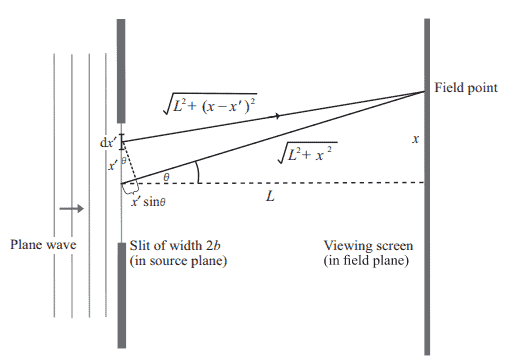
In many cases of interest in optics, Eq. (1.9) is solved to a good approximation by Huygens’ integral. The field is assumed to be known on a “source plane” $S_{1}$ perpendicular to the $z$-axis and is only nonzero in some finite region of that plane. The values of the field on $S_{1}$ serve as a boundary condition for solving Eq. (1.9). The solution is given by Huygens’ integral for the complex scalar field at any desired point $x, y, z$.
$$
\tilde{E}(x, y, z)=\frac{i}{\lambda} \iint_{S_{1}} \tilde{E}\left(x^{\prime}, y^{\prime}, z^{\prime}\right) \cos \phi \frac{e^{-i k r}}{r} \mathrm{~d} S^{\prime} .
$$
The integration over the source plane $S_{1}$ is performed using the integration variables $x^{\prime}$, $y^{\prime}, z^{\prime}$. The vector $\vec{r}$ joins points in the source plane $S_{1}$ with the point $(x, y, z)$ at which we are calculating the field. The angle between $\vec{r}$ and the z-axis is $\phi$ (see Figure 1.1). The solution represented by Huygens’ integral is satisfying because it encapsulates an intuitive understanding of how light waves behave that was understood long before the formal mathematics was fully worked out.
The intuitive description of Eq. (1.10) is known as Huygens’ principle, due to Christiaan Huygens (1629-1695), a Dutch mathematician and scientist. Under Huygens’ principle, every point in the source is considered to be emitting light with spherical wavefronts propagating outward – the so-called Huygens’ wavelets. These wavefronts are represented by the factor $\cos \phi \frac{e^{–i t}}{r}$. They are emitted preferentially in the direction perpendicular to the source plane due to the presence of $\cos \phi$. The constant $\frac{i}{\lambda}$ out-front contributes $90^{\circ}$ of phase and the $\lambda$ in the denominator serves to keep the units the same on both sides of the equation. The complex scalar field in the source plane $E\left(x, y, z_{1}\right)$ sets the relative amplitudes and phases of these tiny spherical emitters. The field $\tilde{F}(x, y, z)$ is then simply the linear superposition of all the spherical wavefronts emitted from the source.
光学代考
物理代写|光学代写Optics代考|Maxwell’s Equations
光学领域描述了光在空间和材料中传播时的行为。为了理解光的行为,我们从描述它的基本经典物理模型开始:
麦克斯韦电动力学方程。麦克斯韦方程表明电场和磁场可以像波一样传播。在无源区域,线性介质中的麦克斯韦 方程组为 $^{1}$
$$
\vec{\nabla} \cdot \vec{E}=0, \vec{\nabla} \cdot \vec{B} \quad=0, \vec{\nabla} \times \vec{E}=-\frac{\partial \vec{B}}{\partial t}, \vec{\nabla} \times \vec{B} \quad=\mu \epsilon \frac{\partial \vec{E}}{\partial t},
$$
在哪里 $\vec{E}$ 是电场, $\vec{B}$ 是磁场, $\mu$ 是介质的渗透率,并且 $\epsilon$ 是介质的介电常数。如果我们取等式两边的卷曲。(1.3)、 应用向量恒等式 $\vec{\nabla} \times \vec{\nabla} \times \vec{E}=\vec{\nabla}(\vec{\nabla} \cdot \vec{E})-\nabla^{2} \vec{E}$ 到左边,交换时间导数的顺序和右边的curl,我们得到
$$
\vec{\nabla}(\vec{\nabla} \cdot \vec{E})-\nabla^{2} \vec{E}=-\frac{\partial(\vec{\nabla} \times \vec{B})}{\partial t}
$$
然后从方程式替换。(1.1)和 (1.4) 得到
$$
\nabla^{2} \vec{E}=\mu \epsilon \frac{\partial^{2} \vec{E}}{\partial t^{2}}
$$
这是波速为的三维波动方程 $v=1 / \sqrt{\mu \epsilon}$. 以方程的卷曲。(1.4) 并执行类似的代数表明,磁场也满足具有相同波速 的波动方程。因此麦克斯韦方程允许电磁波。在真空中,速度为 $v=1 / \sqrt{\mu_{0} \epsilon_{0}} \equiv c$ ,真空中的光速。光确实是 一种电磁波。
我们现在寻找方程的解决方案。(1.6) 及其磁场对应物。我们实际上只需要求解电场,因为磁场总是可以从 $\vec{B}=\frac{1}{c} \hat{k} \times \vec{E}$ ,在哪里 $\hat{k}$ 是行进的方向。
物理代写|光学代写Optics代考|Huygens’ Principle
在许多对光学感兴趣的情况下,方程式。(1.9) 通过惠更斯积分求解到一个很好的近似值。假定该场在“源平面”上 是已知的 $S_{1}$ 垂直于 $z$-轴,并且仅在该平面的某些有限区域中非零。字段的值 $S_{1}$ 作为求解方程的边界条件。(1.9)。 解由惠更斯积分在任何所需点处对复标量场给出 $x, y, z$.
$$
\tilde{E}(x, y, z)=\frac{i}{\lambda} \iint_{S_{1}} \tilde{E}\left(x^{\prime}, y^{\prime}, z^{\prime}\right) \cos \phi \frac{e^{-i k r}}{r} \mathrm{~d} S^{\prime} .
$$
源平面上的集成 $S_{1}$ 使用积分变量执行 $x^{\prime}, y^{\prime}, z^{\prime}$. 向量 $\vec{r}$ 连接源平面中的点 $S_{1}$ 有一点 $(x, y, z)$ 我们正在计算该字 段。之间的角度 $\vec{r}$ z轴是 $\phi$ (见图 1.1) 。惠更斯积分所代表的解决方案是令人满意的,因为它封装了对光波行为方 式的直观理解,这种理解早在正式数学完全解决之前就已被理解。
方程的直观描述。(1.10) 因荷兰数学家和科学家克里斯蒂安.惠更斯 (1629-1695) 而被称为惠更斯原理。根据惠更 斯原理,光源中的每个点都被认为是发射具有向外传播的球形波前的光一一即所谓的惠更斯小波。这些波前由因 子表示 $\cos \phi \frac{e^{-i t}}{r}$. 由于存在 $\cos \phi$. 常数 $\frac{i}{\lambda}$ 前线贡献 $90^{\circ}$ 相位和 $\lambda$ 分母中的单位用于保持等式两边的单位相同。源平 面中的复标量场 $E\left(x, y, z_{1}\right)$ 设置这些微小球形发射器的相对幅度和相位。场 $\tilde{F}(x, y, z)$ 然后是从源发射的所有球面波前的简单线性叠加。

统计代写请认准statistics-lab™. statistics-lab™为您的留学生涯保驾护航。
金融工程代写
金融工程是使用数学技术来解决金融问题。金融工程使用计算机科学、统计学、经济学和应用数学领域的工具和知识来解决当前的金融问题,以及设计新的和创新的金融产品。
非参数统计代写
非参数统计指的是一种统计方法,其中不假设数据来自于由少数参数决定的规定模型;这种模型的例子包括正态分布模型和线性回归模型。
广义线性模型代考
广义线性模型(GLM)归属统计学领域,是一种应用灵活的线性回归模型。该模型允许因变量的偏差分布有除了正态分布之外的其它分布。
术语 广义线性模型(GLM)通常是指给定连续和/或分类预测因素的连续响应变量的常规线性回归模型。它包括多元线性回归,以及方差分析和方差分析(仅含固定效应)。
有限元方法代写
有限元方法(FEM)是一种流行的方法,用于数值解决工程和数学建模中出现的微分方程。典型的问题领域包括结构分析、传热、流体流动、质量运输和电磁势等传统领域。
有限元是一种通用的数值方法,用于解决两个或三个空间变量的偏微分方程(即一些边界值问题)。为了解决一个问题,有限元将一个大系统细分为更小、更简单的部分,称为有限元。这是通过在空间维度上的特定空间离散化来实现的,它是通过构建对象的网格来实现的:用于求解的数值域,它有有限数量的点。边界值问题的有限元方法表述最终导致一个代数方程组。该方法在域上对未知函数进行逼近。[1] 然后将模拟这些有限元的简单方程组合成一个更大的方程系统,以模拟整个问题。然后,有限元通过变化微积分使相关的误差函数最小化来逼近一个解决方案。
tatistics-lab作为专业的留学生服务机构,多年来已为美国、英国、加拿大、澳洲等留学热门地的学生提供专业的学术服务,包括但不限于Essay代写,Assignment代写,Dissertation代写,Report代写,小组作业代写,Proposal代写,Paper代写,Presentation代写,计算机作业代写,论文修改和润色,网课代做,exam代考等等。写作范围涵盖高中,本科,研究生等海外留学全阶段,辐射金融,经济学,会计学,审计学,管理学等全球99%专业科目。写作团队既有专业英语母语作者,也有海外名校硕博留学生,每位写作老师都拥有过硬的语言能力,专业的学科背景和学术写作经验。我们承诺100%原创,100%专业,100%准时,100%满意。
随机分析代写
随机微积分是数学的一个分支,对随机过程进行操作。它允许为随机过程的积分定义一个关于随机过程的一致的积分理论。这个领域是由日本数学家伊藤清在第二次世界大战期间创建并开始的。
时间序列分析代写
随机过程,是依赖于参数的一组随机变量的全体,参数通常是时间。 随机变量是随机现象的数量表现,其时间序列是一组按照时间发生先后顺序进行排列的数据点序列。通常一组时间序列的时间间隔为一恒定值(如1秒,5分钟,12小时,7天,1年),因此时间序列可以作为离散时间数据进行分析处理。研究时间序列数据的意义在于现实中,往往需要研究某个事物其随时间发展变化的规律。这就需要通过研究该事物过去发展的历史记录,以得到其自身发展的规律。
回归分析代写
多元回归分析渐进(Multiple Regression Analysis Asymptotics)属于计量经济学领域,主要是一种数学上的统计分析方法,可以分析复杂情况下各影响因素的数学关系,在自然科学、社会和经济学等多个领域内应用广泛。
MATLAB代写
MATLAB 是一种用于技术计算的高性能语言。它将计算、可视化和编程集成在一个易于使用的环境中,其中问题和解决方案以熟悉的数学符号表示。典型用途包括:数学和计算算法开发建模、仿真和原型制作数据分析、探索和可视化科学和工程图形应用程序开发,包括图形用户界面构建MATLAB 是一个交互式系统,其基本数据元素是一个不需要维度的数组。这使您可以解决许多技术计算问题,尤其是那些具有矩阵和向量公式的问题,而只需用 C 或 Fortran 等标量非交互式语言编写程序所需的时间的一小部分。MATLAB 名称代表矩阵实验室。MATLAB 最初的编写目的是提供对由 LINPACK 和 EISPACK 项目开发的矩阵软件的轻松访问,这两个项目共同代表了矩阵计算软件的最新技术。MATLAB 经过多年的发展,得到了许多用户的投入。在大学环境中,它是数学、工程和科学入门和高级课程的标准教学工具。在工业领域,MATLAB 是高效研究、开发和分析的首选工具。MATLAB 具有一系列称为工具箱的特定于应用程序的解决方案。对于大多数 MATLAB 用户来说非常重要,工具箱允许您学习和应用专业技术。工具箱是 MATLAB 函数(M 文件)的综合集合,可扩展 MATLAB 环境以解决特定类别的问题。可用工具箱的领域包括信号处理、控制系统、神经网络、模糊逻辑、小波、仿真等。