如果你也在 怎样代写最优化Optimization Theory 这个学科遇到相关的难题,请随时右上角联系我们的24/7代写客服。最优化Optimization Theory是致力于解决优化问题的数学分支。 优化问题是我们想要最小化或最大化函数值的数学函数。 这些类型的问题在计算机科学和应用数学中大量存在。
最优化Optimization Theory每个优化问题都包含三个组成部分:目标函数、决策变量和约束。 当人们谈论制定优化问题时,它意味着将“现实世界”问题转化为包含这三个组成部分的数学方程和变量。目标函数,通常表示为 f 或 z,反映要最大化或最小化的单个量。交通领域的例子包括“最小化拥堵”、“最大化安全”、“最大化可达性”、“最小化成本”、“最大化路面质量”、“最小化排放”、“最大化收入”等等。
statistics-lab™ 为您的留学生涯保驾护航 在代写最优化理论optimization theory方面已经树立了自己的口碑, 保证靠谱, 高质且原创的统计Statistics代写服务。我们的专家在代写最优化理论optimization theory代写方面经验极为丰富,各种代写最优化理论optimization theory相关的作业也就用不着说。

数学代写|最优化理论作业代写optimization theory代考|A Continuous Stirred-Tank Chemical Reactor
Example 6.2-2. The state equations for a continuous stirred-tank chemical reactor are given below [L-5]. The flow of a coolant through a coil inserted in the reactor is to control the first-order, irreversible exothermic reaction taking place in the reactor. The states of the plant are $x_1(t)=T(t)$ (the deviation from the steady-state temperature) and $x_2(t)=C(t)$ (the deviation from the steady-state concentration). $u(t)$, the normalized control variable, represents the effect of coolant flow on the chemical reaction. The state equations are
$$
\begin{aligned}
\dot{x}_1(t)= & -2\left[x_1(t)+0.25\right]+\left[x_2(t)+0.5\right] \exp \left[\frac{25 x_1(t)}{x_1(t)+2}\right] \
& -\left[x_1(t)+0.25\right] u(t) \
\dot{x}_2(t)= & 0.5-x_2(t)-\left[x_2(t)+0.5\right] \exp \left[\frac{25 x_1(t)}{x_1(t)+2}\right]
\end{aligned}
$$
with initial conditions $\mathbf{x}(0)=\left[\begin{array}{ll}0.05 & 0\end{array}\right]^T$. The performance measure to be minimized is
$$
J=\int_0^{0.78}\left[x_1^2(t)+x_2^2(t)+R u^2(t)\right] d t,
$$
indicating that the desired objective is to maintain the temperature and concentration close to their steady-state values without expending large amounts of control effort. $R$ is a weighting factor that we shall select (arbitrarily) as 0.1 . The costate equations are determined from the Hamiltonian,
$$
\begin{aligned}
\mathscr{H}(\mathbf{x}(t) & u(t), \mathbf{p}(t))=x_1^2(t)+x_2^2(t)+R u^2(t) \
& +p_1(t)\left[-2\left[x_1(t)+0.25\right]+\left[x_2(t)+0.5\right] \exp \left[\frac{25 x_1(t)}{x_1(t)+2}\right]\right. \
& \left.-\left[x_1(t)+0.25\right] u(t)\right]+p_2(t)\left[0.5-x_2(t)\right. \
& \left.-\left[x_2(t)+0.5\right] \exp \left[\frac{25 x_1(t)}{x_1(t)+2}\right]\right]
\end{aligned}
$$
as
$$
\begin{aligned}
\dot{p}_1(t)= & -\frac{\partial \mathscr{H}}{\partial x_1}=-2 x_1(t)+2 p_1(t) \
& -p_1(t)\left[x_2(t)+0.5\right]\left[\frac{50}{\left[x_1(t)+2\right]^2}\right] \exp \left[\frac{25 x_1(t)}{x_1(t)+2}\right] \
& +p_1(t) u(t)+p_2(t)\left[x_2(t)+0.5\right]\left[\frac{50}{\left[x_1(t)+2\right]^2}\right] \exp \left[\frac{25 x_1(t)}{x_1(t)+2}\right] \
\dot{p}_2(t)= & -\frac{\partial \mathscr{H}}{\partial x_2}=-2 x_2(t)-p_1(t) \exp \left[\frac{25 x_1(t)}{x_1(t)+2}\right] \
& +p_2(t)\left[1+\exp \left[\frac{25 x_1(t)}{x_1(t)+2}\right]\right] .
\end{aligned}
$$
数学代写|最优化理论作业代写optimization theory代考|Features of the Steepest Descent Algorithm
To conclude our discussion of the steepest descent method, let us summarize the important features of the algorithm.
Initial Guess. A nominal control history, $\mathbf{u}^{(0)}(t), t \in\left[t_0, t_f\right]$, must be selected to begin the numerical procedure. In selecting the nominal control we utilize whatever physical insight we have about the problem.
Storage Requirements. The current trial control $\mathbf{u}^{(i)}$, the corresponding state trajectory $\mathbf{x}^{(i)}$, and the gradient history $\partial \mathscr{H}^{(i)} / \partial \mathbf{u}$, are stored. If storage must be conserved, the state values needed to determine $\partial \mathscr{H}^{(t)} / \partial \mathbf{u}$ can be obtained by reintegrating the state equations with the costate equations. If this is done $\mathbf{x}^{(t)}$ does not need to be stored; however, the computation time will increase. Generating the required state values in this manner may make the results of the backward integration more accurate, because the piecewise-constant approximation for $\mathbf{x}^{(l)}$ need not be used.
Convergence. The method of steepest descent is generally characterized by ease of starting – the initial guess for the control is not usually crucial. On the other hand, as a minimum is approached, the gradient becomes small and the method has a tendency to converge slowly.
Computations Required. In each iteration numerical integration of $2 n$ firstorder ordinary differential equations is required. In addition, the time history of $\partial \mathscr{H}^{(t)} / \partial \mathrm{u}$ at the times $t_k, k=0,1, \ldots, N-1$, must be evaluated. To speed up the iterative procedure, a single variable search may be used to determine the step size for the change in the trial control.
Stopping Criterion. The iterative procedure is terminated when a criterion such as $\left|\partial \mathscr{H}^{(i)} / \partial \mathbf{u}\right|<\gamma_1$ or $\left|J^{(i)}-J^{(i+1)}\right|<\gamma_2$ is satisfied; $\gamma_1$ and $\gamma_2$ are preselected positive numbers.
最优化理论代写
数学代写|最优化理论作业代写optimization theory代考|A Continuous Stirred-Tank Chemical Reactor
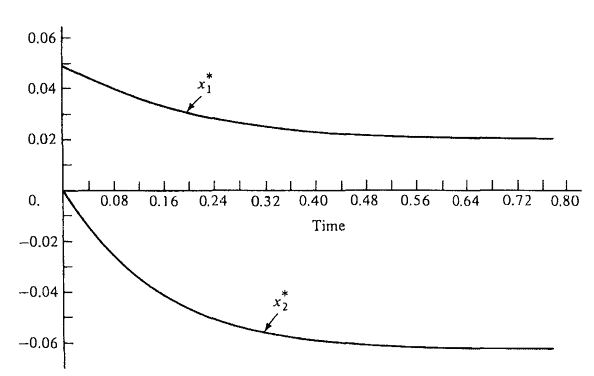
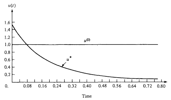
例6.2-2。连续搅拌槽式化学反应器的状态方程如下[L-5]。冷却剂流经插入反应器内的线圈是为了控制发生在反应器内的一级不可逆放热反应。工厂的状态为$x_1(t)=T(t)$(偏离稳态温度)和$x_2(t)=C(t)$(偏离稳态浓度)。归一化控制变量$u(t)$表示冷却剂流量对化学反应的影响。状态方程是
$$
\begin{aligned}
\dot{x}_1(t)= & -2\left[x_1(t)+0.25\right]+\left[x_2(t)+0.5\right] \exp \left[\frac{25 x_1(t)}{x_1(t)+2}\right] \
& -\left[x_1(t)+0.25\right] u(t) \
\dot{x}_2(t)= & 0.5-x_2(t)-\left[x_2(t)+0.5\right] \exp \left[\frac{25 x_1(t)}{x_1(t)+2}\right]
\end{aligned}
$$
有初始条件$\mathbf{x}(0)=\left[\begin{array}{ll}0.05 & 0\end{array}\right]^T$。要最小化的性能度量是
$$
J=\int_0^{0.78}\left[x_1^2(t)+x_2^2(t)+R u^2(t)\right] d t,
$$
表明期望的目标是保持温度和浓度接近其稳态值,而不花费大量的控制努力。$R$是一个权重因子,我们将(任意)选择为0.1。协态方程由哈密顿函数决定,
$$
\begin{aligned}
\mathscr{H}(\mathbf{x}(t) & u(t), \mathbf{p}(t))=x_1^2(t)+x_2^2(t)+R u^2(t) \
& +p_1(t)\left[-2\left[x_1(t)+0.25\right]+\left[x_2(t)+0.5\right] \exp \left[\frac{25 x_1(t)}{x_1(t)+2}\right]\right. \
& \left.-\left[x_1(t)+0.25\right] u(t)\right]+p_2(t)\left[0.5-x_2(t)\right. \
& \left.-\left[x_2(t)+0.5\right] \exp \left[\frac{25 x_1(t)}{x_1(t)+2}\right]\right]
\end{aligned}
$$
as
$$
\begin{aligned}
\dot{p}_1(t)= & -\frac{\partial \mathscr{H}}{\partial x_1}=-2 x_1(t)+2 p_1(t) \
& -p_1(t)\left[x_2(t)+0.5\right]\left[\frac{50}{\left[x_1(t)+2\right]^2}\right] \exp \left[\frac{25 x_1(t)}{x_1(t)+2}\right] \
& +p_1(t) u(t)+p_2(t)\left[x_2(t)+0.5\right]\left[\frac{50}{\left[x_1(t)+2\right]^2}\right] \exp \left[\frac{25 x_1(t)}{x_1(t)+2}\right] \
\dot{p}_2(t)= & -\frac{\partial \mathscr{H}}{\partial x_2}=-2 x_2(t)-p_1(t) \exp \left[\frac{25 x_1(t)}{x_1(t)+2}\right] \
& +p_2(t)\left[1+\exp \left[\frac{25 x_1(t)}{x_1(t)+2}\right]\right] .
\end{aligned}
$$
数学代写|最优化理论作业代写optimization theory代考|Features of the Steepest Descent Algorithm
为了结束对最陡下降法的讨论,让我们总结一下该算法的重要特征。
初步猜测。一个标称的控制历史,$\mathbf{u}^{(0)}(t), t \in\left[t_0, t_f\right]$,必须选择开始数值过程。在选择标称控制时,我们利用我们对问题的任何物理洞察力。
存储要求。存储当前试验控制$\mathbf{u}^{(i)}$,相应的状态轨迹$\mathbf{x}^{(i)}$和梯度历史$\partial \mathscr{H}^{(i)} / \partial \mathbf{u}$。如果必须保留存储空间,则可以通过将状态方程与协态方程重新积分来获得确定$\partial \mathscr{H}^{(t)} / \partial \mathbf{u}$所需的状态值。如果这样做$\mathbf{x}^{(t)}$不需要存储;但是,计算时间会增加。以这种方式生成所需的状态值可以使后向积分的结果更加准确,因为不需要使用$\mathbf{x}^{(l)}$的分段常数近似。
收敛。最陡下降法的一般特点是易于启动——对控制的初始猜测通常并不重要。另一方面,当逼近最小值时,梯度变小,该方法有收敛缓慢的趋势。
需要计算。在每次迭代中,需要对$2 n$一级常微分方程进行数值积分。此外,必须对$\partial \mathscr{H}^{(t)} / \partial \mathrm{u}$在$t_k, k=0,1, \ldots, N-1$时代的时间历史进行评估。为了加快迭代过程,可以使用单变量搜索来确定试验控制中变化的步长。
停止标准。当满足$\left|\partial \mathscr{H}^{(i)} / \partial \mathbf{u}\right|<\gamma_1$或$\left|J^{(i)}-J^{(i+1)}\right|<\gamma_2$等标准时,迭代过程终止;$\gamma_1$和$\gamma_2$是预选的正数。

统计代写请认准statistics-lab™. statistics-lab™为您的留学生涯保驾护航。
金融工程代写
金融工程是使用数学技术来解决金融问题。金融工程使用计算机科学、统计学、经济学和应用数学领域的工具和知识来解决当前的金融问题,以及设计新的和创新的金融产品。
非参数统计代写
非参数统计指的是一种统计方法,其中不假设数据来自于由少数参数决定的规定模型;这种模型的例子包括正态分布模型和线性回归模型。
广义线性模型代考
广义线性模型(GLM)归属统计学领域,是一种应用灵活的线性回归模型。该模型允许因变量的偏差分布有除了正态分布之外的其它分布。
术语 广义线性模型(GLM)通常是指给定连续和/或分类预测因素的连续响应变量的常规线性回归模型。它包括多元线性回归,以及方差分析和方差分析(仅含固定效应)。
有限元方法代写
有限元方法(FEM)是一种流行的方法,用于数值解决工程和数学建模中出现的微分方程。典型的问题领域包括结构分析、传热、流体流动、质量运输和电磁势等传统领域。
有限元是一种通用的数值方法,用于解决两个或三个空间变量的偏微分方程(即一些边界值问题)。为了解决一个问题,有限元将一个大系统细分为更小、更简单的部分,称为有限元。这是通过在空间维度上的特定空间离散化来实现的,它是通过构建对象的网格来实现的:用于求解的数值域,它有有限数量的点。边界值问题的有限元方法表述最终导致一个代数方程组。该方法在域上对未知函数进行逼近。[1] 然后将模拟这些有限元的简单方程组合成一个更大的方程系统,以模拟整个问题。然后,有限元通过变化微积分使相关的误差函数最小化来逼近一个解决方案。
tatistics-lab作为专业的留学生服务机构,多年来已为美国、英国、加拿大、澳洲等留学热门地的学生提供专业的学术服务,包括但不限于Essay代写,Assignment代写,Dissertation代写,Report代写,小组作业代写,Proposal代写,Paper代写,Presentation代写,计算机作业代写,论文修改和润色,网课代做,exam代考等等。写作范围涵盖高中,本科,研究生等海外留学全阶段,辐射金融,经济学,会计学,审计学,管理学等全球99%专业科目。写作团队既有专业英语母语作者,也有海外名校硕博留学生,每位写作老师都拥有过硬的语言能力,专业的学科背景和学术写作经验。我们承诺100%原创,100%专业,100%准时,100%满意。
随机分析代写
随机微积分是数学的一个分支,对随机过程进行操作。它允许为随机过程的积分定义一个关于随机过程的一致的积分理论。这个领域是由日本数学家伊藤清在第二次世界大战期间创建并开始的。
时间序列分析代写
随机过程,是依赖于参数的一组随机变量的全体,参数通常是时间。 随机变量是随机现象的数量表现,其时间序列是一组按照时间发生先后顺序进行排列的数据点序列。通常一组时间序列的时间间隔为一恒定值(如1秒,5分钟,12小时,7天,1年),因此时间序列可以作为离散时间数据进行分析处理。研究时间序列数据的意义在于现实中,往往需要研究某个事物其随时间发展变化的规律。这就需要通过研究该事物过去发展的历史记录,以得到其自身发展的规律。
回归分析代写
多元回归分析渐进(Multiple Regression Analysis Asymptotics)属于计量经济学领域,主要是一种数学上的统计分析方法,可以分析复杂情况下各影响因素的数学关系,在自然科学、社会和经济学等多个领域内应用广泛。
MATLAB代写
MATLAB 是一种用于技术计算的高性能语言。它将计算、可视化和编程集成在一个易于使用的环境中,其中问题和解决方案以熟悉的数学符号表示。典型用途包括:数学和计算算法开发建模、仿真和原型制作数据分析、探索和可视化科学和工程图形应用程序开发,包括图形用户界面构建MATLAB 是一个交互式系统,其基本数据元素是一个不需要维度的数组。这使您可以解决许多技术计算问题,尤其是那些具有矩阵和向量公式的问题,而只需用 C 或 Fortran 等标量非交互式语言编写程序所需的时间的一小部分。MATLAB 名称代表矩阵实验室。MATLAB 最初的编写目的是提供对由 LINPACK 和 EISPACK 项目开发的矩阵软件的轻松访问,这两个项目共同代表了矩阵计算软件的最新技术。MATLAB 经过多年的发展,得到了许多用户的投入。在大学环境中,它是数学、工程和科学入门和高级课程的标准教学工具。在工业领域,MATLAB 是高效研究、开发和分析的首选工具。MATLAB 具有一系列称为工具箱的特定于应用程序的解决方案。对于大多数 MATLAB 用户来说非常重要,工具箱允许您学习和应用专业技术。工具箱是 MATLAB 函数(M 文件)的综合集合,可扩展 MATLAB 环境以解决特定类别的问题。可用工具箱的领域包括信号处理、控制系统、神经网络、模糊逻辑、小波、仿真等。