
如果你也在 怎样代写量子场论Quantum field theory这个学科遇到相关的难题,请随时右上角联系我们的24/7代写客服。
在理论物理学中,量子场论(QFT)是一个理论框架,它结合了经典场论、狭义相对论和量子力学。QFT在粒子物理学中被用来构建亚原子粒子的物理模型,在凝聚态物理学中被用来构建类粒子的模型。
statistics-lab™ 为您的留学生涯保驾护航 在代写量子场论Quantum field theory方面已经树立了自己的口碑, 保证靠谱, 高质且原创的统计Statistics代写服务。我们的专家在代写量子场论Quantum field theory代写方面经验极为丰富,各种代写量子场论Quantum field theory相关的作业也就用不着说。
物理代写|量子场论代写Quantum field theory代考|Position-space Feynman rules
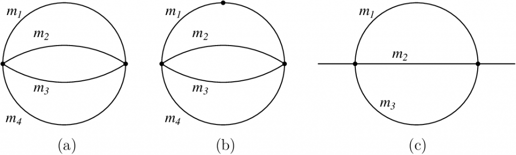
We have shown that the same sets of diagrams appear in the Hamiltonian and the Lagrangian approaches: each point $x_i$ in the original $n$-point function $\langle\Omega| T\left{\phi\left(x_1\right) \cdots\right.$ $\left.\phi\left(x_n\right)\right}|\Omega\rangle$ gets an external point and each interaction gives a new vertex whose position is integrated over and whose coefficient is given by the coefficient in the Lagrangian.
As long as the vertices are normalized with appropriate permutation factors, as in Eq. (7.24), the combinatoric factors will work out the same, as we saw in the example. In the Lagrangian approach, we saw that the coefficient of the diagram will be given by the coefficient of the interaction multiplied by the geometrical symmetry factor of the diagram. To see that this is also true for the Hamiltonian, we have to count the various combinatoric factors:
There is a factor of $\frac{1}{m !}$ from the expansion of $\exp \left(i \mathcal{L}{\text {int }}\right)=\sum \frac{1}{m !}\left(i \mathcal{L}{\text {int }}\right)^m$. If we expand to order $m$ there will be $m$ identical vertices in the same diagram. We can also swap these vertices around, leaving the diagram looking the same. If we only include the diagram once in our final sum, the $m$ ! from permuting the diagrams will cancel the $\frac{1}{m !}$ from the exponential. Neither of these factors were present in the Lagrangian approach,since internal vertices came out of the splitting of lines associated with external vertices, which was unambiguous, and there was no exponential to begin with.
If interactions are normalized as in Eq. (7.24), then there will be a $\frac{1}{j !}$ for each interaction with $j$ identical particles. This factor is canceled by the $j$ ! ways of permuting the $j$ identical lines coming out of the same internal vertex. In the Lagrangian approach, one of the lines was already chosen so the factor was $(j-1)$ !, with the missing $j$ coming from using $\mathcal{L}{\text {int }}^{\prime}[\phi]$ instead of $\mathcal{L}{\text {int }}[\phi]$.
The result is the same Feynman rules as were derived in the Lagrangian approach. In both cases, symmetry factors must be added if there is some geometric symmetry (there rarely is in theories with complex fields, such as QED). In neither case do any of the diagrams include bubbles (subdiagrams that do not connect with any external vertex).
物理代写|量子场论代写Quantum field theory代考|Momentum-space Feynman rules
The position-space Feynman rules derived in either of the previous two sections give a recipe for computing time-ordered products in perturbation theory. Now we will see how those time-ordered products simplify when all the phase-space integrals over the propagators are performed to turn them into $S$-matrix elements. This will produce the momentum-space Feynman rules.
Consider the diagram
$$
\mathcal{T}1=\overbrace{}^{x_1} \overbrace{}^{x_2} \bullet=-\frac{g^2}{2} \int d^4 x \int d^4 y D{1 x} D_{x y}^2 D_{y 2} .
$$
To evaluate this diagram, first write every propagator in momentum space (taking $m=0$ for simplicity):
$$
D_{x y}=\int \frac{d^4 p}{(2 \pi)^4} \frac{i}{p^2+i \varepsilon} e^{i p(x-y)}
$$
Then there will be four $d^4 p$ integrals from the four propagators and all the positions will appear only in exponentials. So,
$$
\begin{aligned}
\mathcal{T}_1= & -\frac{g^2}{2} \int d^4 x \int d^4 y \int \frac{d^4 p_1}{(2 \pi)^4} \int \frac{d^4 p_2}{(2 \pi)^4} \int \frac{d^4 p_3}{(2 \pi)^4} \int \frac{d^4 p_4}{(2 \pi)^4} \
& \times e^{i p_1\left(x_1-x\right)} e^{i p_2\left(y-x_2\right)} e^{i p_3(x-y)} e^{i p_4(x-y)} \frac{i}{p_1^2+i \varepsilon} \frac{i}{p_2^2+i \varepsilon} \frac{i}{p_3^2+i \varepsilon} \frac{i}{p_4^2+i \varepsilon}
\end{aligned}
$$
Now we can do the $x$ and $y$ integrals, which produce $\delta^4\left(-p_1+p_3+p_4\right)$ and $\delta^4\left(p_2-p_3-p_4\right)$ respectively, corresponding to momentum being conserved at the vertices labeled $x$ and $y$ in the Feynman diagram. If we integrate over $p_3$ using the first $\delta$-function then we can replace $p_3=p_1-p_4$ and the second $\delta$-function becomes $\delta^4\left(p_1-p_2\right)$. Then we have, relabeling $p_4=k$,
$$
\begin{aligned}
& \mathcal{T}_1=-\frac{\lambda^2}{2} \int \frac{d^4 k}{(2 \pi)^4} \int \frac{d^4 p_1}{(2 \pi)^4} \int \frac{d^4 p_2}{(2 \pi)^4} e^{i p_1 x_1} e^{-i p_2 x_2} \
& \times \frac{i}{p_1^2+i \varepsilon} \frac{i}{p_2^2+i \varepsilon} \frac{i}{\left(p_1-k\right)^2+i \varepsilon} \frac{i}{k^2+i \varepsilon}(2 \pi)^4 \delta^4\left(p_1-p_2\right)
\end{aligned}
$$
Next, we use the LSZ formula to convert this to a contribution to the $S$-matrix:
$$
\langle f|S| i\rangle=\left[-i \int d^4 x_1 e^{-i p_i x_1}\left(p_i^2\right)\right]\left[-i \int d^4 x_2 e^{i p_f x_2}\left(p_f^2\right)\right]\left\langle\Omega\left|T\left{\phi\left(x_1\right) \phi\left(x_2\right)\right}\right| \Omega\right\rangle,
$$
where $p_i^\mu$ and $p_f^\mu$ are the initial state and final state momenta. So the contribution of this diagram gives
$$
\langle f|S| i\rangle=-\int d^4 x_1 e^{-i p_i x_1}\left(p_i\right)^2 \int d^4 x_2 e^{i p_f x_2}\left(p_f^2\right) \mathcal{T}_1+\cdots
$$
量子场论代考
物理代写|量子场论代写Quantum field theory代考|Position-space Feynman rules
我们已经证明,在哈密顿方法和拉格朗日方法中出现了相同的图集:原始$n$ -point函数$\langle\Omega| T\left{\phi\left(x_1\right) \cdots\right.$$\left.\phi\left(x_n\right)\right}|\Omega\rangle$中的每个点$x_i$得到一个外部点,每个相互作用给出一个新的顶点,其位置被积分,其系数由拉格朗日系数给出。
只要用适当的排列因子对顶点进行归一化,如Eq.(7.24)所示,组合因子将得到相同的结果,如我们在示例中看到的那样。在拉格朗日方法中,我们看到图的系数将由相互作用系数乘以图的几何对称系数给出。为了证明这对哈密顿函数也是成立的,我们必须计算各种组合因子:
有一个因子$\frac{1}{m !}$来自于$\exp \left(i \mathcal{L}{\text {int }}\right)=\sum \frac{1}{m !}\left(i \mathcal{L}{\text {int }}\right)^m$的扩展。如果我们将其展开为$m$,那么在同一个图中就会有$m$个相同的顶点。我们也可以交换这些顶点,让图看起来一样。如果我们在最终的总和中只包含一次图表,那么$m$ !通过排列图表可以把$\frac{1}{m !}$从指数中消去。这两个因素在拉格朗日方法中都不存在,因为内部顶点来自与外部顶点相关的线的分裂,这是明确的,并且没有指数开始。
如果相互作用如式(7.24)中所示归一化,那么与$j$相同粒子的每个相互作用将有一个$\frac{1}{j !}$。这个因子被$j$ !排列$j$从同一个内部顶点出来的相同直线的方法。在拉格朗日方法中,已经选择了一条直线,因此因子是$(j-1)$ !,而缺少的$j$来自使用$\mathcal{L}{\text {int }}^{\prime}[\phi]$而不是$\mathcal{L}{\text {int }}[\phi]$。
其结果与在拉格朗日方法中导出的费曼规则相同。在这两种情况下,如果存在一些几何对称性,就必须添加对称因子(在具有复杂场的理论中,例如QED,很少有对称因子)。在这两种情况下,任何图表都不包括气泡(不与任何外部顶点连接的子图表)。
物理代写|量子场论代写Quantum field theory代考|Momentum-space Feynman rules
在前两节中导出的位置空间费曼规则给出了在微扰理论中计算时间顺序积的方法。现在我们将看到这些时间顺序的乘积是如何简化的当对传播量进行相空间积分将它们变成$S$ -矩阵元素。这就产生了动量空间费曼规则。
考虑这个图
$$
\mathcal{T}1=\overbrace{}^{x_1} \overbrace{}^{x_2} \bullet=-\frac{g^2}{2} \int d^4 x \int d^4 y D{1 x} D_{x y}^2 D_{y 2} .
$$
为了评估这个图,首先写出动量空间中的每个传播子(为了简单起见,取$m=0$):
$$
D_{x y}=\int \frac{d^4 p}{(2 \pi)^4} \frac{i}{p^2+i \varepsilon} e^{i p(x-y)}
$$
然后会有四个$d^4 p$积分来自四个传播算子所有的位置只会出现在指数中。所以,
$$
\begin{aligned}
\mathcal{T}_1= & -\frac{g^2}{2} \int d^4 x \int d^4 y \int \frac{d^4 p_1}{(2 \pi)^4} \int \frac{d^4 p_2}{(2 \pi)^4} \int \frac{d^4 p_3}{(2 \pi)^4} \int \frac{d^4 p_4}{(2 \pi)^4} \
& \times e^{i p_1\left(x_1-x\right)} e^{i p_2\left(y-x_2\right)} e^{i p_3(x-y)} e^{i p_4(x-y)} \frac{i}{p_1^2+i \varepsilon} \frac{i}{p_2^2+i \varepsilon} \frac{i}{p_3^2+i \varepsilon} \frac{i}{p_4^2+i \varepsilon}
\end{aligned}
$$
现在我们可以做$x$和$y$积分,它们分别产生$\delta^4\left(-p_1+p_3+p_4\right)$和$\delta^4\left(p_2-p_3-p_4\right)$,对应于费曼图中标记为$x$和$y$的顶点处的动量守恒。如果我们使用第一个$\delta$ -函数对$p_3$进行积分,那么我们可以替换$p_3=p_1-p_4$,而第二个$\delta$ -函数变成$\delta^4\left(p_1-p_2\right)$。然后我们重新标记$p_4=k$,
$$
\begin{aligned}
& \mathcal{T}_1=-\frac{\lambda^2}{2} \int \frac{d^4 k}{(2 \pi)^4} \int \frac{d^4 p_1}{(2 \pi)^4} \int \frac{d^4 p_2}{(2 \pi)^4} e^{i p_1 x_1} e^{-i p_2 x_2} \
& \times \frac{i}{p_1^2+i \varepsilon} \frac{i}{p_2^2+i \varepsilon} \frac{i}{\left(p_1-k\right)^2+i \varepsilon} \frac{i}{k^2+i \varepsilon}(2 \pi)^4 \delta^4\left(p_1-p_2\right)
\end{aligned}
$$
接下来,我们使用LSZ公式将其转换为对$S$ -矩阵的贡献:
$$
\langle f|S| i\rangle=\left[-i \int d^4 x_1 e^{-i p_i x_1}\left(p_i^2\right)\right]\left[-i \int d^4 x_2 e^{i p_f x_2}\left(p_f^2\right)\right]\left\langle\Omega\left|T\left{\phi\left(x_1\right) \phi\left(x_2\right)\right}\right| \Omega\right\rangle,
$$
其中$p_i^\mu$和$p_f^\mu$是初始态动量和末态动量。这张图的作用是
$$
\langle f|S| i\rangle=-\int d^4 x_1 e^{-i p_i x_1}\left(p_i\right)^2 \int d^4 x_2 e^{i p_f x_2}\left(p_f^2\right) \mathcal{T}_1+\cdots
$$

统计代写请认准statistics-lab™. statistics-lab™为您的留学生涯保驾护航。
金融工程代写
金融工程是使用数学技术来解决金融问题。金融工程使用计算机科学、统计学、经济学和应用数学领域的工具和知识来解决当前的金融问题,以及设计新的和创新的金融产品。
非参数统计代写
非参数统计指的是一种统计方法,其中不假设数据来自于由少数参数决定的规定模型;这种模型的例子包括正态分布模型和线性回归模型。
广义线性模型代考
广义线性模型(GLM)归属统计学领域,是一种应用灵活的线性回归模型。该模型允许因变量的偏差分布有除了正态分布之外的其它分布。
术语 广义线性模型(GLM)通常是指给定连续和/或分类预测因素的连续响应变量的常规线性回归模型。它包括多元线性回归,以及方差分析和方差分析(仅含固定效应)。
有限元方法代写
有限元方法(FEM)是一种流行的方法,用于数值解决工程和数学建模中出现的微分方程。典型的问题领域包括结构分析、传热、流体流动、质量运输和电磁势等传统领域。
有限元是一种通用的数值方法,用于解决两个或三个空间变量的偏微分方程(即一些边界值问题)。为了解决一个问题,有限元将一个大系统细分为更小、更简单的部分,称为有限元。这是通过在空间维度上的特定空间离散化来实现的,它是通过构建对象的网格来实现的:用于求解的数值域,它有有限数量的点。边界值问题的有限元方法表述最终导致一个代数方程组。该方法在域上对未知函数进行逼近。[1] 然后将模拟这些有限元的简单方程组合成一个更大的方程系统,以模拟整个问题。然后,有限元通过变化微积分使相关的误差函数最小化来逼近一个解决方案。
tatistics-lab作为专业的留学生服务机构,多年来已为美国、英国、加拿大、澳洲等留学热门地的学生提供专业的学术服务,包括但不限于Essay代写,Assignment代写,Dissertation代写,Report代写,小组作业代写,Proposal代写,Paper代写,Presentation代写,计算机作业代写,论文修改和润色,网课代做,exam代考等等。写作范围涵盖高中,本科,研究生等海外留学全阶段,辐射金融,经济学,会计学,审计学,管理学等全球99%专业科目。写作团队既有专业英语母语作者,也有海外名校硕博留学生,每位写作老师都拥有过硬的语言能力,专业的学科背景和学术写作经验。我们承诺100%原创,100%专业,100%准时,100%满意。
随机分析代写
随机微积分是数学的一个分支,对随机过程进行操作。它允许为随机过程的积分定义一个关于随机过程的一致的积分理论。这个领域是由日本数学家伊藤清在第二次世界大战期间创建并开始的。
时间序列分析代写
随机过程,是依赖于参数的一组随机变量的全体,参数通常是时间。 随机变量是随机现象的数量表现,其时间序列是一组按照时间发生先后顺序进行排列的数据点序列。通常一组时间序列的时间间隔为一恒定值(如1秒,5分钟,12小时,7天,1年),因此时间序列可以作为离散时间数据进行分析处理。研究时间序列数据的意义在于现实中,往往需要研究某个事物其随时间发展变化的规律。这就需要通过研究该事物过去发展的历史记录,以得到其自身发展的规律。
回归分析代写
多元回归分析渐进(Multiple Regression Analysis Asymptotics)属于计量经济学领域,主要是一种数学上的统计分析方法,可以分析复杂情况下各影响因素的数学关系,在自然科学、社会和经济学等多个领域内应用广泛。
MATLAB代写
MATLAB 是一种用于技术计算的高性能语言。它将计算、可视化和编程集成在一个易于使用的环境中,其中问题和解决方案以熟悉的数学符号表示。典型用途包括:数学和计算算法开发建模、仿真和原型制作数据分析、探索和可视化科学和工程图形应用程序开发,包括图形用户界面构建MATLAB 是一个交互式系统,其基本数据元素是一个不需要维度的数组。这使您可以解决许多技术计算问题,尤其是那些具有矩阵和向量公式的问题,而只需用 C 或 Fortran 等标量非交互式语言编写程序所需的时间的一小部分。MATLAB 名称代表矩阵实验室。MATLAB 最初的编写目的是提供对由 LINPACK 和 EISPACK 项目开发的矩阵软件的轻松访问,这两个项目共同代表了矩阵计算软件的最新技术。MATLAB 经过多年的发展,得到了许多用户的投入。在大学环境中,它是数学、工程和科学入门和高级课程的标准教学工具。在工业领域,MATLAB 是高效研究、开发和分析的首选工具。MATLAB 具有一系列称为工具箱的特定于应用程序的解决方案。对于大多数 MATLAB 用户来说非常重要,工具箱允许您学习和应用专业技术。工具箱是 MATLAB 函数(M 文件)的综合集合,可扩展 MATLAB 环境以解决特定类别的问题。可用工具箱的领域包括信号处理、控制系统、神经网络、模糊逻辑、小波、仿真等。