statistics-lab™ 为您的留学生涯保驾护航在代写回归分析Regression Analysis方面已经树立了自己的口碑, 保证靠谱, 高质且原创的统计Statistics代写服务。我们的专家在代写回归分析Regression Analysis代写方面经验极为丰富，各种代写回归分析Regression Analysis相关的作业也就用不着说。

统计代写|回归分析作业代写Regression Analysis代考|Simulation Study to Understand the Null Distribution of the $T$ Statistic

The following $\mathrm{R}$ code generates the data under the null model. It is the same model used in the SSN/Height example above, but re-written in a way to make the constraint $\beta_1=0$ explicit. Because we did not use set.seed as in the previous code, the output is random. Your results will differ, but that is good because the point here is to understand randomness.

$\mathrm{n}=100$
beta $0=70 ;$ betal $=0 \quad #$ The null model; true betal = 0
ssn = sample $(0: 9,100$, replace=T)
height = beta + betal*ssn + rnorm $(100,0,4)$
ssn.data = data.frame (ssn, height)
fit. $1=$ lm (height ssn, data=ssn.data)
summary (fit. 1$)$
$\mathrm{n}=100$
beta $0=70 ;$ betal $=0 \quad #$ The null model; true betal $=0$
ssn $=$ sample $(0: 9,100$, replace $=T)$
height $=$ beta $0+\operatorname{beta} 1 * \operatorname{ssn}+\operatorname{rnorm}(100,0,4)$
ssn. data = data. frame (ssn, height)
fit. 1 = $\operatorname{lm}($ height ssn, datasssn. data)
summary (fit.l)
This code gives the following output (yours will vary by randomness):
Cal :
$\operatorname{lm}$ (formula $=$ height $\sim$ ssn, data $=$ ssn. data)
Residuals:
Min $1 Q$ Median $3 Q$ Max
$-9.4952-2.8261-0.3936 \quad 2.252111 .6764$
Coefficients :
Estimate std. Error $t$ value $\operatorname{Pr}(>|t|)$
(Intercept) $69.77372 \quad 0.71865 \quad 97.089<2 \mathrm{e}-16 \star \star $ $\operatorname{ssn} 0.019150 .14336 \quad 0.134 \quad 0.894$ Signif. Codes: 0 ‘‘ 0.001 ‘‘ 0.01 ‘*’ 0.05 ‘. 0.1 ‘ 1
Residual standard error: 4.155 on 98 degrees of freedom
Multiple R-squared: 0.000182 , Adjusted R-squared: 0.01002
F-statistic: 0.01784 on 1 and $98 \mathrm{DF}$, p-value: 0.894
In our simulation, the estimate $\hat{\beta}_1=0.01915$ is $T=0.134$ standard errors from zero, and you know that this difference is explained by chance alone because the data are simulated from the null model where $\beta_1=0$.

统计代写|回归分析作业代写Regression Analysis代考|The $p$-Value

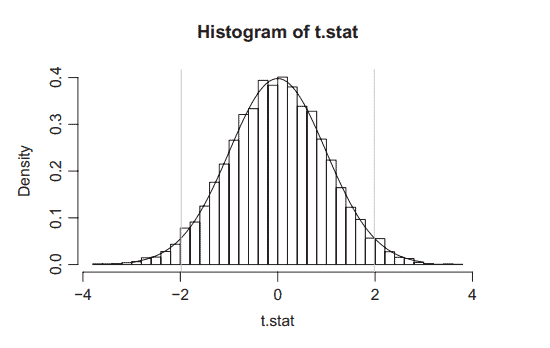
In the example above, the thresholds to determine which real $T$ values are explainable by chance alone are the numbers that put $95 \%$ of the $T$ values that are explained by chance alone between them; these are -1.9845 and +1.9845 in the case of the $T_{98}$ distribution. If the observed $T$ statistic falls outside that range, then we can say that the difference between $\hat{\beta}_1$ and 0 is not easily explained by chance alone.

See Figure 3.7 again. Notice that there is $5 \%$ total probability outside the \pm 1.9845 range, simply because there is $95 \%$ probability inside the range. Now, if the $T$ statistic falls inside the $95 \%$ range, then there has to be more than $5 \%$ total probability outside the $\pm T$ range. See Figure 3.7 again, and suppose $T=1.7$, which is inside the range. Then there has to be more than $5 \%$ probability outside the \pm 1.7 range, right? See Figure 3.7 again, and locate \pm 1.7 on the graph. Make sure you understand this; it is not hard at all. Do not just read the words, because then you will not understand. Instead, look at Figure 3.7, put your finger on the graph at 1.7 , and think about the area outside the \pm 1.7 range. It is more than 0.05 , do you see?

Now, suppose $T=2.5$, and look at Figure 3.7 again. Then there has to be less than $5 \%$ probability outside the \pm 2.5 range, right? See Figure 3.7 again, and locate \pm 2.5 on the graph. Make sure you understand this; it is not hard at all. Look at the graph! Do not just read the words! Instead, put your finger on the graph at 2.5 and think about the area outside the \pm 2.5 range. It is less than 0.05 , do you see?

回归分析代写

统计代写|回归分析作业代写Regression Analysis代考|Simulation Study to Understand the Null Distribution of the $T$ Statistic

下面的$\mathrm{R}$代码生成null模型下的数据。它与上面的SSN/Height示例中使用的模型相同，但是以一种使约束$\beta_1=0$显式的方式重新编写。因为我们没有用集合。与前面的代码一样，输出是随机的。你的结果可能会有所不同，但这很好，因为这里的重点是理解随机性。

$\mathrm{n}=100$
beta $0=70 ;$ betal $=0 \quad #$ null模型;True betal = 0
ssn = sample $(0: 9,100$, replace=T)
高度= beta + beta *ssn + rnorm $(100,0,4)$
ssn. ssn.Data = Data .frame (ssn, height)
适合。$1=$ lm(高度ssn，数据=ssn.data)
总结(适合)1 $)$
$\mathrm{n}=100$
beta $0=70 ;$ betal $=0 \quad #$ null模型;真betal $=0$
SSN $=$样例$(0: 9,100$，替换$=T)$
身高$=$ beta $0+\operatorname{beta} 1 * \operatorname{ssn}+\operatorname{rnorm}(100,0,4)$
ssn. ssn.数据=数据。框架(ssn, height)
适合。1 = $\operatorname{lm}($ height ssn, datasssn。数据)
摘要(fit. 1)
这段代码给出了以下输出(你的输出会随随机而变化):
卡尔:
$\operatorname{lm}$(公式$=$高度$\sim$ ssn，数据$=$ ssn。数据)
残差:
最小值$1 Q$中值$3 Q$最大值
$-9.4952-2.8261-0.3936 \quad 2.252111 .6764$
系数:
估计std误差$t$值$\operatorname{Pr}(>|t|)$
(截音)$69.77372 \quad 0.71865 \quad 97.089<2 \mathrm{e}-16 \star \star $$\operatorname{ssn} 0.019150 .14336 \quad 0.134 \quad 0.894$代码:0“0.001”“0.01”*“0.05”。0.1 ‘ 1
剩余标准误差:在98自由度上为4.155
多元r平方:0.000182，调整r平方:0.01002
f统计量:0.01784对1和$98 \mathrm{DF}$, p值:0.894
在我们的模拟中，估计值$\hat{\beta}_1=0.01915$是$T=0.134$离零的标准误差，并且您知道这种差异完全是偶然的，因为数据是从null模型模拟的，其中$\beta_1=0$。

统计代写|回归分析作业代写Regression Analysis代考|The $p$-Value

在上面的例子中，确定哪些真实的$T$值只能由偶然解释的阈值是将只能由偶然解释的$T$值中的$95 \%$放在它们之间的数字;在$T_{98}$分布的情况下，它们是-1.9845和+1.9845。如果观察到的$T$统计值超出了这个范围，那么我们可以说$\hat{\beta}_1$和0之间的差异不容易单独用偶然来解释。

再次参见图3.7。注意，在\pm 1.9845范围之外有$5 \%$总概率，因为在范围内有$95 \%$概率。现在，如果$T$统计值落在$95 \%$范围内，那么在$\pm T$范围外的总概率必须大于$5 \%$。再次参见图3.7，假设$T=1.7$在范围内。那么在\pm 1.7范围之外的概率必须大于$5 \%$，对吧?再次参见图3.7，并在图中找到\pm 1.7。确保你理解了这一点;这一点也不难。不要只看文字，因为那样你不会明白。相反，请查看图3.7，将手指放在1.7处的图形上，并考虑\pm 1.7范围之外的区域。它大于0.05，你看到了吗?

现在，假设$T=2.5$，再次查看图3.7。那么在\pm 2.5范围之外的概率必须小于$5 \%$，对吧?再次参见图3.7，在图中找到\pm 2.5。确保你理解了这一点;这一点也不难。看这个图表!不要只看单词!相反，将手指放在2.5的图形上，并考虑\pm 2.5范围之外的区域。它小于0.05，你看到了吗?

统计代写|回归分析作业代写Regression Analysis代考请认准statistics-lab™

统计代写请认准statistics-lab™. statistics-lab™为您的留学生涯保驾护航。

随机过程代考

在概率论概念中，随机过程是随机变量的集合。若一随机系统的样本点是随机函数，则称此函数为样本函数，这一随机系统全部样本函数的集合是一个随机过程。实际应用中，样本函数的一般定义在时间域或者空间域。 随机过程的实例如股票和汇率的波动、语音信号、视频信号、体温的变化，随机运动如布朗运动、随机徘徊等等。

贝叶斯方法代考

贝叶斯统计概念及数据分析表示使用概率陈述回答有关未知参数的研究问题以及统计范式。后验分布包括关于参数的先验分布，和基于观测数据提供关于参数的信息似然模型。根据选择的先验分布和似然模型，后验分布可以解析或近似，例如，马尔科夫链蒙特卡罗 (MCMC) 方法之一。贝叶斯统计概念及数据分析使用后验分布来形成模型参数的各种摘要，包括点估计，如后验平均值、中位数、百分位数和称为可信区间的区间估计。此外，所有关于模型参数的统计检验都可以表示为基于估计后验分布的概率报表。

广义线性模型代考

广义线性模型（GLM）归属统计学领域，是一种应用灵活的线性回归模型。该模型允许因变量的偏差分布有除了正态分布之外的其它分布。

statistics-lab作为专业的留学生服务机构，多年来已为美国、英国、加拿大、澳洲等留学热门地的学生提供专业的学术服务，包括但不限于Essay代写，Assignment代写，Dissertation代写，Report代写，小组作业代写，Proposal代写，Paper代写，Presentation代写，计算机作业代写，论文修改和润色，网课代做，exam代考等等。写作范围涵盖高中，本科，研究生等海外留学全阶段，辐射金融，经济学，会计学，审计学，管理学等全球99%专业科目。写作团队既有专业英语母语作者，也有海外名校硕博留学生，每位写作老师都拥有过硬的语言能力，专业的学科背景和学术写作经验。我们承诺100%原创，100%专业，100%准时，100%满意。

机器学习代写

随着AI的大潮到来，Machine Learning逐渐成为一个新的学习热点。同时与传统CS相比，Machine Learning在其他领域也有着广泛的应用，因此这门学科成为不仅折磨CS专业同学的“小恶魔”，也是折磨生物、化学、统计等其他学科留学生的“大魔王”。学习Machine learning的一大绊脚石在于使用语言众多，跨学科范围广，所以学习起来尤其困难。但是不管你在学习Machine Learning时遇到任何难题，StudyGate专业导师团队都能为你轻松解决。

多元统计分析代考

基础数据: $N$ 个样本， $P$ 个变量数的单样本，组成的横列的数据表
变量定性: 分类和顺序；变量定量：数值
数学公式的角度分为: 因变量与自变量

时间序列分析代写

随机过程，是依赖于参数的一组随机变量的全体，参数通常是时间。随机变量是随机现象的数量表现，其时间序列是一组按照时间发生先后顺序进行排列的数据点序列。通常一组时间序列的时间间隔为一恒定值（如1秒，5分钟，12小时，7天，1年），因此时间序列可以作为离散时间数据进行分析处理。研究时间序列数据的意义在于现实中，往往需要研究某个事物其随时间发展变化的规律。这就需要通过研究该事物过去发展的历史记录，以得到其自身发展的规律。