如果你也在 怎样代写随机过程stochastic process这个学科遇到相关的难题,请随时右上角联系我们的24/7代写客服。
随机过程 用于表示在时间上发展的统计现象以及在处理这些现象时出现的理论模型,由于这些现象在许多领域都会遇到,因此这篇文章具有广泛的实际意义。
statistics-lab™ 为您的留学生涯保驾护航 在代写随机过程stochastic process方面已经树立了自己的口碑, 保证靠谱, 高质且原创的统计Statistics代写服务。我们的专家在代写随机过程stochastic process代写方面经验极为丰富,各种代写随机过程stochastic process相关的作业也就用不着说。
我们提供的随机过程stochastic process及其相关学科的代写,服务范围广, 其中包括但不限于:
- Statistical Inference 统计推断
- Statistical Computing 统计计算
- Advanced Probability Theory 高等概率论
- Advanced Mathematical Statistics 高等数理统计学
- (Generalized) Linear Models 广义线性模型
- Statistical Machine Learning 统计机器学习
- Longitudinal Data Analysis 纵向数据分析
- Foundations of Data Science 数据科学基础
统计代写|随机过程代写stochastic process代考|Hexagonal Lattice, Nearest Neighbors
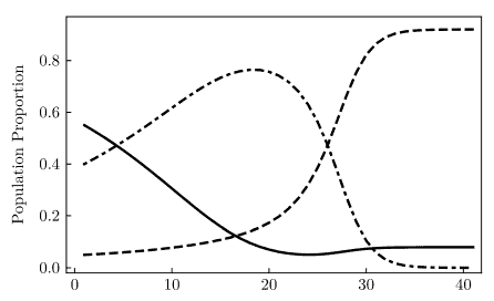
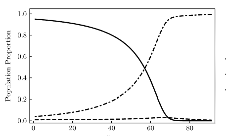
Here I dive into the details of the processes discussed in Section 1.5.3. I also discuss Figure 2. The source code to produce Figure 2 is discussed in Sections $6.4$ (nearest neighbor graph) and $6.7$ (visualizations). Some elements of graph theory are discussed here, as well as visualization techniques.
Surprisingly, it is possible to produce a point process with a regular hexagonal lattice space using simple operations on a small number $(m=4)$ of square lattices: superimposition, stretching, and shifting. A stretched lattice is a square lattice turned into a rectangular lattice, by applying a multiplication factor to the $\mathrm{X}$ and/or Y coordinates. A shifted lattice is a lattice where the grid points have been shifted via a translation.
Each point of the process almost surely (with probability one) has exactly one nearest neighbor. However, when the scaling factor $s$ is zero, this is no longer true. On the left plot in Figure 2, each point (also called vertex when $s=0$ ) has exactly 3 nearest neighbors. This causes some challenges when plotting the case $s=0$. The case $s>0$ is easier to plot, using arrows pointing from any point to its unique nearest neighbor. I produced the arrows in question with the arrow function in R, see source code in Section $6.7$, and online documentation here. $\mathrm{A}$ bidirectional arrow between points $\mathrm{A}$ and $\mathrm{B}$ means that $\mathrm{B}$ is a nearest neighbor of $\mathrm{A}$, and $\mathrm{A}$ is a nearest neighbor of B. All arrows on the left plot in Figure 2 are bidirectional. Boundary effects are easily noticeable, as some arrows point to nearest neighbors outside the window. Four colors are used for the points, corresponding to the 4 shifted stretched Poisson-binomial processes used to generate the hexagon-based process. The color indicates which of these 4 process, a point is attached to.
The source code in Section $6.4$ handles points with multiple nearest neighbors. It produces a list of all points with their nearest neighbors, using a hash table. A point with 3 nearest neighbors has 3 entries in that list: one for each nearest neighbor. A group of points that are all connected by arrows, is called a connected component [Wiki]. A path from a point of a connected component to another point of the same connected component, following arrows while ignoring their direction, is called a path in graph theory.
In my definition of connected component, the direction of the arrow does not matter: the underlying graph is considered undirected [Wiki]. An interesting problem is to study the size distribution, that is, the number of points per connected component, especially for standard Poisson processes. See Exercise 20. In graph theory, a point is called a vertex or node, and an arrow is called an edge. More about nearest neighbors is discussed in Exercises 18 and 19.
Finally, if you look at Figure 2, the left plot seems to have more points than the right plot. But they actually have roughly the same number of points. The plot on the right seems to be more sparse, because there are large areas with no points. But to compensate, there are areas where several points are in close proximity.
统计代写|随机过程代写stochastic process代考|Modeling Cluster Systems in Two Dimensions
There are various ways to create points scattered around a center. When multiple centers are involved, we get a cluster structure. The point process consisting of the centers is called the parent process, while the point distribution around each center, is called the child process. So we are dealing with a two-layer, or hierarchical structure, referred to as a cluster point process. Besides clustering, many other types of point process operations [Wiki] are possible when combining two processes, such as thinning or superimposition. Typical examples of cluster point processes include Neyma-Scott (see here) and Matérn (see here).
Useful references include Baddeley’s textbook “Spatial Point Processes and their Applications” [4] available online here, Sigman’s course material (Columbia University) on one-dimensional renewal processes for beginners, entitled “Notes on the Poisson Process” [71], available online here, Last and Kenrose’s book “Lectures on the Poisson Process” [52], and Cressie’s comprehensive 900-page book “Statistics for Spatial Data” [16]. Cluster point processes are part of a larger field known as spatial statistics, encompassing other techniques such as geostatistics, kriging and tessellations. For lattice-based processes known as perturbed lattice point processes, more closely related to the theme of this textbook (lattice processes), and also more recent with applications to cellular networks, see the following references:
- “On Comparison of Clustering Properties of Point Processes” [12]. Online PDF here.
- “Clustering and percolation of point processes” [11]. Online version here.
- “Clustering comparison of point processes, applications to random geometric models” [13]. Online version here.
- “Stochastic Geometry-Based Tools for Spatial Modeling and Planning of Future Cellular Networks” [51]. Online version here.
- “Hyperuniform and rigid stable matchings” [54]. Online PDF here. Short presentation available here.
- “Rigidity and tolerance for perturbed lattices” [68]. Online version here.
- “Cluster analysis of spatial point patterns: posterior distribution of parents inferred from offspring” [66].
- “Recovering the lattice from its random perturbations” [79]. Online version here.
- “Geometry and Topology of the Boolean Model on a Stationary Point Processes” [81]. Online version here.
- “On distances between point patterns and their applications” [56]. Online version here.
More general references include two comprehensive volumes on point process theory by Daley and Vere-Jones [20, 21], a chapter by Johnson [45] (available online here or here), books by Møller and Waagepetersen, focusing on statistical inference for spatial processes [60, 61], and “Point Pattern Analysis: Nearest Neighbor Statistics” by Anselin [3] focusing on point inhibition/aggregation metrics, available here. See also [58] by Møller, available online here, and “Limit Theorems for Network Dependent Random Variables” [48], available online here.
随机过程代考
统计代写|随机过程代写stochastic process代考|Hexagonal Lattice, Nearest Neighbors
在这里,我将深入探讨第 1.5.3 节中讨论的过程的细节。我还讨论了图 2。生成图 2 的源代码在章节中讨论6.4(最近邻图)和6.7(可视化)。这里讨论了图论的一些元素,以及可视化技术。
令人惊讶的是,可以使用对小数的简单操作来产生具有正六边形格子空间的点过程(米=4)方格:叠加、拉伸和移动。拉伸点阵是通过将乘法因子应用到X和/或 Y 坐标。移位点阵是其中网格点已通过平移移位的点阵。
该过程的每个点几乎肯定(概率为 1)恰好有一个最近的邻居。然而,当比例因子秒为零,这不再是真的。在图 2 的左侧图中,每个点(也称为顶点秒=0) 正好有 3 个最近的邻居。这在策划案件时会带来一些挑战秒=0. 案子秒>0更容易绘制,使用从任何点指向其唯一最近邻居的箭头。我用 R 中的箭头函数生成了有问题的箭头,请参阅部分中的源代码6.7, 以及此处的在线文档。一种点之间的双向箭头一种和乙意思是乙是的最近邻一种, 和一种是 B 的最近邻居。图 2 中左侧图中的所有箭头都是双向的。边界效应很容易被注意到,因为一些箭头指向窗外最近的邻居。这些点使用四种颜色,对应于用于生成基于六边形的过程的 4 个移位拉伸泊松二项式过程。颜色表示这 4 个过程中的哪一个,一个点被附加到。
节中的源代码6.4处理具有多个最近邻居的点。它使用哈希表生成所有点及其最近邻居的列表。具有 3 个最近邻居的点在该列表中有 3 个条目:每个最近邻居一个。一组全部由箭头连接的点,称为连通分量 [Wiki]。从连通分量的一点到同一连通分量的另一点的路径,沿着箭头而忽略其方向,在图论中称为路径。
在我对连通分量的定义中,箭头的方向无关紧要:底层图被认为是无向的 [Wiki]。一个有趣的问题是研究大小分布,即每个连通分量的点数,特别是对于标准泊松过程。参见练习 20。在图论中,点称为顶点或节点,箭头称为边。更多关于最近邻的内容在练习 18 和 19 中讨论。
最后,如果您查看图 2,左边的图似乎比右边的图有更多的点。但他们实际上拥有大致相同的点数。右边的图似乎更稀疏,因为有大片区域没有点。但为了补偿,有些区域的几个点非常接近。
统计代写|随机过程代写stochastic process代考|Modeling Cluster Systems in Two Dimensions
有多种方法可以创建散布在中心周围的点。当涉及多个中心时,我们得到一个集群结构。由中心组成的点进程称为父进程,而围绕每个中心分布的点称为子进程。因此,我们正在处理一个双层或层次结构,称为聚类点过程。除了聚类,许多其他类型的点过程操作 [Wiki] 在组合两个过程时也是可能的,例如细化或叠加。聚类点过程的典型示例包括 Neyma-Scott(参见此处)和 Matérn(参见此处)。
有用的参考资料包括 Baddeley 的教科书“Spatial Point Processes and their Applications”[4],可在此处在线获取,Sigman 的一维更新过程初学者课程材料(哥伦比亚大学),标题为“泊松过程注释”[71],可在线获取在这里,Last 和 Kenrose 的著作“泊松过程讲座”[52],以及 Cressie 的 900 页综合著作“空间数据统计”[16]。聚类点过程是称为空间统计的更大领域的一部分,包括其他技术,例如地质统计学、克里金法和曲面细分。对于称为扰动格点过程的基于格的过程,与本教科书的主题(格过程)更密切相关,并且最近与蜂窝网络的应用有关,请参阅以下参考资料:
- 《论点过程的聚类特性比较》[12]。此处为在线 PDF。
- “点过程的聚类和渗透”[11]。在线版本在这里。
- “点过程的聚类比较,在随机几何模型中的应用”[13]。在线版本在这里。
- “用于未来蜂窝网络空间建模和规划的基于随机几何的工具”[51]。在线版本在这里。
- “超均匀和刚性稳定匹配”[54]。此处为在线 PDF。此处提供简短演示。
- “扰动格子的刚度和容忍度”[68]。在线版本在这里。
- “空间点模式的聚类分析:从后代推断出父母的后验分布”[66]。
- “从随机扰动中恢复晶格”[79]。在线版本在这里。
- “驻点过程布尔模型的几何和拓扑”[81]。在线版本在这里。
- “关于点模式之间的距离及其应用”[56]。在线版本在这里。
更一般的参考资料包括 Daley 和 Vere-Jones [20, 21] 的两本关于点过程理论的综合性著作,Johnson [45] 的一章(可在此处或此处在线获取),Møller 和 Waagepetersen 的书籍,侧重于空间的统计推断过程 [60、61] 和 Anselin [3] 的“点模式分析:最近邻统计”重点关注点抑制/聚合指标,可在此处获取。另请参见 Møller 的 [58],可在此处在线获取,以及“网络相关随机变量的极限定理”[48],可在此处在线获取。

统计代写请认准statistics-lab™. statistics-lab™为您的留学生涯保驾护航。
金融工程代写
金融工程是使用数学技术来解决金融问题。金融工程使用计算机科学、统计学、经济学和应用数学领域的工具和知识来解决当前的金融问题,以及设计新的和创新的金融产品。
非参数统计代写
非参数统计指的是一种统计方法,其中不假设数据来自于由少数参数决定的规定模型;这种模型的例子包括正态分布模型和线性回归模型。
广义线性模型代考
广义线性模型(GLM)归属统计学领域,是一种应用灵活的线性回归模型。该模型允许因变量的偏差分布有除了正态分布之外的其它分布。
术语 广义线性模型(GLM)通常是指给定连续和/或分类预测因素的连续响应变量的常规线性回归模型。它包括多元线性回归,以及方差分析和方差分析(仅含固定效应)。
有限元方法代写
有限元方法(FEM)是一种流行的方法,用于数值解决工程和数学建模中出现的微分方程。典型的问题领域包括结构分析、传热、流体流动、质量运输和电磁势等传统领域。
有限元是一种通用的数值方法,用于解决两个或三个空间变量的偏微分方程(即一些边界值问题)。为了解决一个问题,有限元将一个大系统细分为更小、更简单的部分,称为有限元。这是通过在空间维度上的特定空间离散化来实现的,它是通过构建对象的网格来实现的:用于求解的数值域,它有有限数量的点。边界值问题的有限元方法表述最终导致一个代数方程组。该方法在域上对未知函数进行逼近。[1] 然后将模拟这些有限元的简单方程组合成一个更大的方程系统,以模拟整个问题。然后,有限元通过变化微积分使相关的误差函数最小化来逼近一个解决方案。
tatistics-lab作为专业的留学生服务机构,多年来已为美国、英国、加拿大、澳洲等留学热门地的学生提供专业的学术服务,包括但不限于Essay代写,Assignment代写,Dissertation代写,Report代写,小组作业代写,Proposal代写,Paper代写,Presentation代写,计算机作业代写,论文修改和润色,网课代做,exam代考等等。写作范围涵盖高中,本科,研究生等海外留学全阶段,辐射金融,经济学,会计学,审计学,管理学等全球99%专业科目。写作团队既有专业英语母语作者,也有海外名校硕博留学生,每位写作老师都拥有过硬的语言能力,专业的学科背景和学术写作经验。我们承诺100%原创,100%专业,100%准时,100%满意。
随机分析代写
随机微积分是数学的一个分支,对随机过程进行操作。它允许为随机过程的积分定义一个关于随机过程的一致的积分理论。这个领域是由日本数学家伊藤清在第二次世界大战期间创建并开始的。
时间序列分析代写
随机过程,是依赖于参数的一组随机变量的全体,参数通常是时间。 随机变量是随机现象的数量表现,其时间序列是一组按照时间发生先后顺序进行排列的数据点序列。通常一组时间序列的时间间隔为一恒定值(如1秒,5分钟,12小时,7天,1年),因此时间序列可以作为离散时间数据进行分析处理。研究时间序列数据的意义在于现实中,往往需要研究某个事物其随时间发展变化的规律。这就需要通过研究该事物过去发展的历史记录,以得到其自身发展的规律。
回归分析代写
多元回归分析渐进(Multiple Regression Analysis Asymptotics)属于计量经济学领域,主要是一种数学上的统计分析方法,可以分析复杂情况下各影响因素的数学关系,在自然科学、社会和经济学等多个领域内应用广泛。
MATLAB代写
MATLAB 是一种用于技术计算的高性能语言。它将计算、可视化和编程集成在一个易于使用的环境中,其中问题和解决方案以熟悉的数学符号表示。典型用途包括:数学和计算算法开发建模、仿真和原型制作数据分析、探索和可视化科学和工程图形应用程序开发,包括图形用户界面构建MATLAB 是一个交互式系统,其基本数据元素是一个不需要维度的数组。这使您可以解决许多技术计算问题,尤其是那些具有矩阵和向量公式的问题,而只需用 C 或 Fortran 等标量非交互式语言编写程序所需的时间的一小部分。MATLAB 名称代表矩阵实验室。MATLAB 最初的编写目的是提供对由 LINPACK 和 EISPACK 项目开发的矩阵软件的轻松访问,这两个项目共同代表了矩阵计算软件的最新技术。MATLAB 经过多年的发展,得到了许多用户的投入。在大学环境中,它是数学、工程和科学入门和高级课程的标准教学工具。在工业领域,MATLAB 是高效研究、开发和分析的首选工具。MATLAB 具有一系列称为工具箱的特定于应用程序的解决方案。对于大多数 MATLAB 用户来说非常重要,工具箱允许您学习和应用专业技术。工具箱是 MATLAB 函数(M 文件)的综合集合,可扩展 MATLAB 环境以解决特定类别的问题。可用工具箱的领域包括信号处理、控制系统、神经网络、模糊逻辑、小波、仿真等。