如果你也在 怎样代写数据可视化Data visualization这个学科遇到相关的难题，请随时右上角联系我们的24/7代写客服。

数据可视化是将信息转化为视觉背景的做法，如地图或图表，使数据更容易被人脑理解并从中获得洞察力。数据可视化的主要目标是使其更容易在大型数据集中识别模式、趋势和异常值。

statistics-lab™ 为您的留学生涯保驾护航 在代写数据可视化Data visualization方面已经树立了自己的口碑, 保证靠谱, 高质且原创的统计Statistics代写服务。我们的专家在代写数据可视化Data visualization代写方面经验极为丰富，各种代写数据可视化Data visualization相关的作业也就用不着说。

我们提供的数据可视化Data visualization及其相关学科的代写，服务范围广, 其中包括但不限于:

• Statistical Inference 统计推断
• Statistical Computing 统计计算
• Advanced Probability Theory 高等概率论
• Advanced Mathematical Statistics 高等数理统计学
• (Generalized) Linear Models 广义线性模型
• Statistical Machine Learning 统计机器学习
• Longitudinal Data Analysis 纵向数据分析
• Foundations of Data Science 数据科学基础

统计代写|数据可视化代写Data visualization代考|Statistical Concepts

Because the present book focuses on regression analysis, it’s helpful to be familiar with basic statistical concepts and terms. Don’t worry: each model explored in this book will be interpreted in detail, and we will revisit most concepts as we go along. These are some of the most important terms we will use throughout this book: p-values, effect sizes, confidence intervals, and standard errors. This section provides a brief (and applied) review of these concepts. Bear in mind that we will simply review the concepts for now. Later we will revisit them in $\mathrm{R}$, so don’t worry if you don’t know how to actually find $p$-values or confidence intervals: we will get to that very soon.

Before we proceed, it’s important to review two basic concepts, namely, samples and populations. Statistical inference is based on the assumption that we can estimate characteristics of populations by randomly ${ }^{1}$ sampling from them. When we collect data from 20 second language learners of English whose first language is Spanish (i.e., our sample), we wish to infer something about all learners who fit that description-that is, the entire population, to which we will never have access. At the end of chapter 2, we will see how to simulate some data and verify how representative a sample is of a given population.

Throughout this book, much like in everyday research, we will analyze samples of data and will infer population parameters from sample parameters. You may be familiar with the different symbols we use to represent these two sets of parameters, but if you’re not, here they are: we calculate the sample mean $(\bar{x})$ to infer the population mean $(\mu)$; we calculate the sample standard deviation $(s)$ to infer the population standard deviation $(\sigma)$. Finally, our sample size $(n)$ is contrasted with the population size $(N)$.

统计代写|数据可视化代写Data visualization代考|p-Values

The notion of a $p$-value is associated with the notion of a null hypothesis $\left(H_{0}\right)$, for example that there’s no difference between the means of two groups. $p$-values are everywhere, and we all know about the magical number: $0.05$. Simply put, $p$-values mean the probability of finding data at least as extreme as the data we haveassuming that the null hypothesis is true. ${ }^{2}$ Simply put, they measure the extent to which a statistical result can be attributed to chance. For example, if we compare the test scores of two groups of learners and we find a low (=significant) $p$-value $(p=0.04)$, we reject the null hypothesis that the mean scores between the groups are the same. We then conclude that these two groups indeed come from different populations, that is, their scores are statistically different because the probability of observing the difference in question if chance alone generated the data is too low given our arbitrarily set threshold of $5 \%$.

How many times have you heard or read that a $p$-value is the probability that the null hypothesis is true? This is perhaps one of the most common misinterpretations of $p$-values-the most common on the list of Greenland et al. (2016). This interpretation is incorrect because $p$-values assume that the null hypothesis is true: low $p$-values indicate that the data is not close to what the null hypothesis predicted they should be; high(er) $p$-values indicate that the data is more or less what we should expect, given what the null hypothesis predicts.

统计代写|数据可视化代写Data visualization代考|Effect Sizes

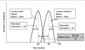
Effect sizes tell us how large the effect of a given variable is on the response variable. There are different ways to measure such effects. If you are familiar with $t$-tests and ANOVAs, you may remember that Cohen’s $d$ and $\eta^{2}$ are two ways to calculate effect sizes. In the models discussed in this book, effect sizes will be given as coefficients, or $\hat{\beta}$ values. The larger a $\hat{\beta}$ value is, the larger the effect size.

Here’s a simple example that shows how effect sizes should be the center of our attention most of the time. Suppose you are interested in recording your classes and making them available to your students. That will require a lot of time and work, but your hypothesis is that by doing so, you will positively affect your students’ learning. You then decide to test it, measuring their learning progress on the basis of their grades. You divide students into two groups. The control group (let’s call it $\mathcal{C}$ ) will not have access to recorded classes, whereas the treatment group $(\mathcal{T})$ will. Each group has 100 students (our sample size), who were randomly assigned to either $\mathcal{C}$ or $\mathcal{T}$ at the beginning of the term. Assuming that all important variables are controlled for, you then spend the entire term on your research project.

At the end of the term, you analyze the groups’ grades and find that the mean grade for group $\mathcal{C}$ was $83.05$ and the mean grade for group $\mathcal{T}$ was $85.11$. Let’s assume that both groups come from populations that have the same standard deviation $(s=3)$. You run a simple statistical test and find a significant result $(p$ $<0.0001)$. Should you conclude that recording all classes was worth it? If you only consider $p$-values, the answer is certainly yes-indeed, given that we are simulating the groups here, we can be sure that they do come from different populations. But take into consideration that the difference between the two groups was only $2.06$ points (over 100) -sure, this tiny difference could mean going from a B+ to an A depending on how generous you are with your grading policy, but let’s ignore that here. Clearly, the effect size here should at least make you question whether all the hours invested in recording all of your classes were worth it.

数据可视化代考

统计代写|数据可视化代写Data visualization代考|Statistical Concepts

因为本书侧重于回归分析，所以熟悉基本的统计概念和术语会很有帮助。别担心：本书中探讨的每个模型都将得到详细解释，并且我们将在进行过程中重新审视大多数概念。这些是我们将在本书中使用的一些最重要的术语：p 值、效应大小、置信区间和标准误。本节提供了对这些概念的简要（和应用）回顾。请记住，我们现在将仅回顾这些概念。稍后我们将在R，所以如果您不知道如何实际找到，请不要担心p-值或置信区间：我们很快就会做到这一点。

在我们继续之前，重要的是要回顾两个基本概念，即样本和总体。统计推断是基于我们可以随机估计种群特征的假设1从他们身上取样。当我们从 20 位第一语言是西班牙语的英语第二语言学习者（即我们的样本）中收集数据时，我们希望推断出所有符合该描述的学习者的信息——即我们永远无法访问的整个人群. 在第 2 章的最后，我们将看到如何模拟一些数据并验证样本在给定总体中的代表性。

在本书中，就像在日常研究中一样，我们将分析数据样本并从样本参数中推断总体参数。您可能熟悉我们用来表示这两组参数的不同符号，但如果您不熟悉，它们就是：我们计算样本均值(X¯)推断总体均值(μ); 我们计算样本标准差(s)推断总体标准差(σ). 最后，我们的样本量(n)与人口规模对比(ñ).

统计代写|数据可视化代写Data visualization代考|p-Values

一个概念p-value 与零假设的概念相关联(H0)，例如两组的平均值之间没有差异。p-值无处不在，我们都知道神奇的数字：0.05. 简单的说，p-值意味着找到数据的概率至少与我们假设零假设为真的数据一样极端。2简而言之，它们衡量统计结果可归因于偶然性的程度。例如，如果我们比较两组学习者的考试成绩，我们发现一个低（=显着）p-价值(p=0.04)，我们拒绝组间平均分数相同的原假设。然后我们得出结论，这两组确实来自不同的人群，也就是说，他们的分数在统计上是不同的，因为如果我们任意设定的阈值，如果仅凭机会生成数据，观察到相关差异的概率太低了。5%.

你听过或读过多少次p-value 是原假设为真的概率？这可能是最常见的误解之一p-values-格陵兰等人列表中最常见的值。（2016 年）。这种解释是不正确的，因为p-values 假设原假设为真：低p-值表明数据与原假设预测的数据不接近；更高）p-值表明数据或多或少是我们应该预期的，给定零假设的预测。

统计代写|数据可视化代写Data visualization代考|Effect Sizes

效应大小告诉我们给定变量对响应变量的影响有多大。有不同的方法来衡量这种影响。如果你熟悉吨-测试和方差分析，你可能还记得科恩的d和这2是计算效果大小的两种方法。在本书讨论的模型中，效应大小将作为系数给出，或者b^价值观。较大的一个b^值越大，效果越大。

这是一个简单的示例，它显示了效果大小在大多数情况下应该如何成为我们关注的中心。假设您有兴趣录制您的课程并将其提供给您的学生。这将需要大量时间和工作，但您的假设是，这样做会对学生的学习产生积极影响。然后，您决定对其进行测试，根据他们的成绩衡量他们的学习进度。你把学生分成两组。对照组（我们称之为C) 将无法访问记录的课程，而治疗组(吨)将要。每组有 100 名学生（我们的样本量），他们被随机分配到C或者吨在学期开始时。假设所有重要变量都得到控制，那么您将整个学期都花在您的研究项目上。

在学期末，您分析小组的成绩并发现小组的平均成绩C曾是83.05和小组的平均成绩吨曾是85.11. 假设两组都来自具有相同标准差的人群(s=3). 您运行一个简单的统计测试并找到一个显着的结果(p <0.0001). 您是否应该得出结论，记录所有课程是值得的？如果只考虑p-values，答案肯定是肯定的——确实，鉴于我们在这里模拟了这些群体，我们可以确定它们确实来自不同的人群。但考虑到两组之间的差异只是2.06分数（超过 100 分）——当然，这个微小的差异可能意味着从 B+ 到 A，这取决于您对评分政策的慷慨程度，但我们在这里忽略这一点。显然，这里的效果大小至少应该让你质疑花在录制所有课程上的所有时间是否值得。

统计代写请认准statistics-lab™. statistics-lab™为您的留学生涯保驾护航。

金融工程代写

金融工程是使用数学技术来解决金融问题。金融工程使用计算机科学、统计学、经济学和应用数学领域的工具和知识来解决当前的金融问题，以及设计新的和创新的金融产品。

非参数统计代写

非参数统计指的是一种统计方法，其中不假设数据来自于由少数参数决定的规定模型；这种模型的例子包括正态分布模型和线性回归模型。

广义线性模型代考

广义线性模型（GLM）归属统计学领域，是一种应用灵活的线性回归模型。该模型允许因变量的偏差分布有除了正态分布之外的其它分布。

术语 广义线性模型（GLM）通常是指给定连续和/或分类预测因素的连续响应变量的常规线性回归模型。它包括多元线性回归，以及方差分析和方差分析（仅含固定效应）。

有限元方法代写

有限元方法（FEM）是一种流行的方法，用于数值解决工程和数学建模中出现的微分方程。典型的问题领域包括结构分析、传热、流体流动、质量运输和电磁势等传统领域。

有限元是一种通用的数值方法，用于解决两个或三个空间变量的偏微分方程（即一些边界值问题）。为了解决一个问题，有限元将一个大系统细分为更小、更简单的部分，称为有限元。这是通过在空间维度上的特定空间离散化来实现的，它是通过构建对象的网格来实现的：用于求解的数值域，它有有限数量的点。边界值问题的有限元方法表述最终导致一个代数方程组。该方法在域上对未知函数进行逼近。[1] 然后将模拟这些有限元的简单方程组合成一个更大的方程系统，以模拟整个问题。然后，有限元通过变化微积分使相关的误差函数最小化来逼近一个解决方案。

tatistics-lab作为专业的留学生服务机构，多年来已为美国、英国、加拿大、澳洲等留学热门地的学生提供专业的学术服务，包括但不限于Essay代写，Assignment代写，Dissertation代写，Report代写，小组作业代写，Proposal代写，Paper代写，Presentation代写，计算机作业代写，论文修改和润色，网课代做，exam代考等等。写作范围涵盖高中，本科，研究生等海外留学全阶段，辐射金融，经济学，会计学，审计学，管理学等全球99%专业科目。写作团队既有专业英语母语作者，也有海外名校硕博留学生，每位写作老师都拥有过硬的语言能力，专业的学科背景和学术写作经验。我们承诺100%原创，100%专业，100%准时，100%满意。

随机分析代写

随机微积分是数学的一个分支，对随机过程进行操作。它允许为随机过程的积分定义一个关于随机过程的一致的积分理论。这个领域是由日本数学家伊藤清在第二次世界大战期间创建并开始的。

时间序列分析代写

随机过程，是依赖于参数的一组随机变量的全体，参数通常是时间。 随机变量是随机现象的数量表现，其时间序列是一组按照时间发生先后顺序进行排列的数据点序列。通常一组时间序列的时间间隔为一恒定值（如1秒，5分钟，12小时，7天，1年），因此时间序列可以作为离散时间数据进行分析处理。研究时间序列数据的意义在于现实中，往往需要研究某个事物其随时间发展变化的规律。这就需要通过研究该事物过去发展的历史记录，以得到其自身发展的规律。

回归分析代写

多元回归分析渐进（Multiple Regression Analysis Asymptotics）属于计量经济学领域，主要是一种数学上的统计分析方法，可以分析复杂情况下各影响因素的数学关系，在自然科学、社会和经济学等多个领域内应用广泛。

MATLAB代写

MATLAB 是一种用于技术计算的高性能语言。它将计算、可视化和编程集成在一个易于使用的环境中，其中问题和解决方案以熟悉的数学符号表示。典型用途包括：数学和计算算法开发建模、仿真和原型制作数据分析、探索和可视化科学和工程图形应用程序开发，包括图形用户界面构建MATLAB 是一个交互式系统，其基本数据元素是一个不需要维度的数组。这使您可以解决许多技术计算问题，尤其是那些具有矩阵和向量公式的问题，而只需用 C 或 Fortran 等标量非交互式语言编写程序所需的时间的一小部分。MATLAB 名称代表矩阵实验室。MATLAB 最初的编写目的是提供对由 LINPACK 和 EISPACK 项目开发的矩阵软件的轻松访问，这两个项目共同代表了矩阵计算软件的最新技术。MATLAB 经过多年的发展，得到了许多用户的投入。在大学环境中，它是数学、工程和科学入门和高级课程的标准教学工具。在工业领域，MATLAB 是高效研究、开发和分析的首选工具。MATLAB 具有一系列称为工具箱的特定于应用程序的解决方案。对于大多数 MATLAB 用户来说非常重要，工具箱允许您学习和应用专业技术。工具箱是 MATLAB 函数（M 文件）的综合集合，可扩展 MATLAB 环境以解决特定类别的问题。可用工具箱的领域包括信号处理、控制系统、神经网络、模糊逻辑、小波、仿真等。

R语言代写	问卷设计与分析代写
PYTHON代写	回归分析与线性模型代写
MATLAB代写	方差分析与试验设计代写
STATA代写	机器学习/统计学习代写
SPSS代写	计量经济学代写
EVIEWS代写	时间序列分析代写
EXCEL代写	深度学习代写
SQL代写	各种数据建模与可视化代写

如果你也在 怎样代写数据可视化Data visualization这个学科遇到相关的难题，请随时右上角联系我们的24/7代写客服。

数据可视化是将信息转化为视觉背景的做法，如地图或图表，使数据更容易被人脑理解并从中获得洞察力。数据可视化的主要目标是使其更容易在大型数据集中识别模式、趋势和异常值。

statistics-lab™ 为您的留学生涯保驾护航 在代写数据可视化Data visualization方面已经树立了自己的口碑, 保证靠谱, 高质且原创的统计Statistics代写服务。我们的专家在代写数据可视化Data visualization代写方面经验极为丰富，各种代写数据可视化Data visualization相关的作业也就用不着说。

我们提供的数据可视化Data visualization及其相关学科的代写，服务范围广, 其中包括但不限于:

• Statistical Inference 统计推断
• Statistical Computing 统计计算
• Advanced Probability Theory 高等概率论
• Advanced Mathematical Statistics 高等数理统计学
• (Generalized) Linear Models 广义线性模型
• Statistical Machine Learning 统计机器学习
• Longitudinal Data Analysis 纵向数据分析
• Foundations of Data Science 数据科学基础

统计代写|数据可视化代写Data visualization代考|Main Objectives of This Book

It goes without saying that the field of second language acquisition (SLA), or second language research more generally, relies on data: test scores, reaction times, grammaticality judgements, certainty levels, categorical preferences, suppliance rates, and so on. Indeed, by the end of the 1990 s, over $90 \%$ of all studies in applied linguistics were quantitative (Cunnings 2012). Different theories have been proposed to explain acquisition patterns that are observed in the data and to predict patterns in unobserved data. To evaluate the validity of any claim in the field, theoretical or not, we must consider empirical evidence, that is, data-much like any scientific field. It is therefore unsurprising that most of what we assume and propose in the field depends on how we analyze our data and, perhaps even more importantly, on how carefully we interpret and generalize the patterns that we find. More often than not, inappropriate analyses lead to incorrect conclusions.

It has been noted in the literature that the field of second language acquisition relies on a precariously narrow range of statistical techniques to quantitatively analyze data (Plonsky 2013, 2014, 2015). $\boldsymbol{t}$-tests and ANOVAs still seem to be the most popular statistical options, even though they are (i) underpowered and (ii) often inappropriate given the data at hand, as will be discussed in Part III. As examples of (i), t-tests can’t handle multiple variables (or groups), and ANOVAs can’t handle complex hierarchical structures in the data (chapter 9), which are essential given how much variation we observe in linguistic data. In addition, both methods focus on $p$-values, not on effect sizes. An example of (ii) would include the use of ANOVAs when we are dealing with binary or scalar responses (chapters 7 and 8 ) – see Jaeger (2008).

统计代写|数据可视化代写Data visualization代考|Why Focus on Data Visualization Techniques

Good figures are crucial. When we want to see and understand the data patterns underlying a study, a figure is likely the best option we have. Whether or not you consider yourself a visual person, the truth is that a well-designed plot almost always communicates your results more effectively than huge tables or a series of numbers and percentages within the body of the text. An appropriate figure can help the reader understand your thinking process, your narrative, and your statistical results-needless to say, you want your reader (or your reviewer) to understand exactly what you mean.

Besides helping the reader, figures help us, the researchers. To design the right figure, we must have a clear understanding of the message we want to

communicate, the pattern we want to focus on. Often times, it is by designing a figure that we realize that we don’t know exactly what we want to see-or that we don’t understand the type of data we are trying to visualize. In that way, data visualization can also improve our thinking process.

Despite the importance of data visualization, it is not uncommon to come across experimental papers in L2 research with very limited figures. How many times have you seen pie charts in papers? Or maybe bar plots without error bars? Perhaps a plot showing variables that do not match the variables discussed later, in the actual analysis? As we will see throughout this book, some general “rules of thumb” can already drastically improve one’s data visualization techniques.

统计代写|数据可视化代写Data visualization代考|Why Focus on Full-Fledged Statistical Models

Data can be messy, and language data almost always is-especially when we deal with L2 research, where multiple grammars can be at play, generating multiple patterns that often seem contradictory. Different leamers behave differently, and they may respond differently to different stimuli or circumstances. On top of all that, we know that multiple variables can play a role in different phenomena. We naturally want to focus on a particular variable of interest, but we shouldn’t ignore potential confounding factors that could also affect our results.

In the past, comparing two groups and concluding that they were statistically different was often good enough. Take $t$-tests, for example, which are usually used when we focus our attention on a single question: are two groups (i.e., means) statistically different? The answer is categorically defined based on an arbitrary number: $0.05$ (see review on $p$-values in $₫ 1.3 .1$ ). This approach often doesn’t care about how different the groups are-although this seems to be more and more a characteristic of the past now (i.e., what is generally referred to as old statistics). In contrast, the focus of statistical analyses these days has shifted a lot in many areas. We now typically focus on models with multiple variables because we wish to estimate the effect $(\$ 1.3 .2$ ) that such variables have on an outcome of interest.

Statistical models are very different from a simple $t$-test. They allow us to incorporate a high degree of complexity and therefore provide more realistic and reliable results. We can, for example, take into account how much learners will vary when it comes to the effect we are examining in our study. By default, such models also provide effect sizes, which are more relevant than mere $p$ values (cf. ANOVAs and $t$-tests, which require additional steps to yield effect sizes). They also allow us to measure the effect of multiple variables-not just one. These are only a few reasons that you should always favor a fullfledged statistical model over statistical tests-or simple ANOVAs, which are technically a special type of a statistical model (linear regression). By focusing on such models, this book provides a powerful, flexible, and up-to-date approach to data analysis.

数据可视化代考

统计代写|数据可视化代写Data visualization代考|Main Objectives of This Book

毋庸置疑，第二语言习得 (SLA) 领域或更普遍的第二语言研究依赖于数据：测试分数、反应时间、语法判断、确定性水平、分类偏好、请求率等。事实上，到 1990 年代末，超过90%应用语言学的所有研究都是定量的（Cunnings 2012）。已经提出了不同的理论来解释在数据中观察到的采集模式并预测未观察到的数据中的模式。为了评估该领域任何主张的有效性，无论是否是理论上的，我们都必须考虑经验证据，即数据——就像任何科学领域一样。因此，我们在该领域的大部分假设和建议都取决于我们如何分析我们的数据，甚至更重要的是，取决于我们如何仔细地解释和概括我们发现的模式，这并不奇怪。不恰当的分析往往会导致错误的结论。

在文献中已经注意到，第二语言习得领域依赖于范围极窄的统计技术来定量分析数据（Plonsky 2013, 2014, 2015）。吨- 检验和 ANOVA 似乎仍然是最流行的统计选项，尽管它们 (i) 能力不足并且 (ii) 考虑到手头的数据通常不合适，正如将在第三部分中讨论的那样。作为 (i) 的示例，t 检验不能处理多个变量（或组），而 ANOVA 不能处理数据中的复杂层次结构（第 9 章），考虑到我们在语言数据中观察到的变化量，这是必不可少的. 此外，这两种方法都侧重于p-值，而不是效果大小。(ii) 的一个例子包括在我们处理二元或标量响应时使用 ANOVA（第 7 章和第 8 章）——参见 Jaeger (2008)。

统计代写|数据可视化代写Data visualization代考|Why Focus on Data Visualization Techniques

好的数字很关键。当我们想要查看和理解研究背后的数据模式时，数字可能是我们拥有的最佳选择。不管你是否认为自己是一个视觉型的人，事实是一个精心设计的情节几乎总是比巨大的表格或文本正文中的一系列数字和百分比更有效地传达你的结果。一个合适的数字可以帮助读者理解你的思考过程、你的叙述和你的统计结果——不用说，你希望你的读者（或你的评论者）准确地理解你的意思。

除了帮助读者，数字也帮助我们，研究人员。要设计正确的图形，我们必须清楚地了解我们想要传达的信息

沟通，我们想要关注的模式。很多时候，通过设计一个图形，我们意识到我们并不确切地知道我们想看到什么——或者我们不了解我们试图可视化的数据类型。这样，数据可视化也可以改善我们的思维过程。

尽管数据可视化很重要，但在 L2 研究中遇到数据非常有限的实验论文并不少见。您在论文中看到过多少次饼图？或者可能是没有误差线的条形图？也许在实际分析中显示的变量与后面讨论的变量不匹配？正如我们将在本书中看到的那样，一些通用的“经验法则”已经可以极大地改进一个人的数据可视化技术。

统计代写|数据可视化代写Data visualization代考|Why Focus on Full-Fledged Statistical Models

数据可能是混乱的，语言数据几乎总是如此——尤其是当我们处理 L2 研究时，可能会出现多种语法，从而产生多种看似矛盾的模式。不同的学习者表现不同，他们可能对不同的刺激或环境做出不同的反应。最重要的是，我们知道多个变量可以在不同的现象中发挥作用。我们自然希望关注特定的感兴趣变量，但我们不应该忽视也可能影响我们结果的潜在混杂因素。

过去，比较两组并得出统计差异的结论通常就足够了。拿吨例如，当我们将注意力集中在一个问题上时，通常会使用测试：两组（即均值）在统计上是否不同？答案是根据任意数字分类定义的：0.05（见评论p-值在₫₫1.3.1）。这种方法通常不关心组的不同程度——尽管现在这似乎越来越成为过去的特征（即，通常称为旧统计数据）。相比之下，如今统计分析的重点在许多领域发生了很大变化。我们现在通常关注具有多个变量的模型，因为我们希望估计效果($1.3.2) 这些变量对感兴趣的结果有影响。

统计模型与简单的模型有很大不同吨-测试。它们使我们能够整合高度的复杂性，从而提供更现实和可靠的结果。例如，当涉及到我们在研究中检查的效果时，我们可以考虑到学习者会有多少变化。默认情况下，此类模型还提供效果大小，这比单纯的更相关p值（参见方差分析和吨-tests，这需要额外的步骤来产生效果大小）。它们还使我们能够衡量多个变量的影响——而不仅仅是一个变量。这些只是您应该始终支持成熟的统计模型而不是统计测试或简单的方差分析的几个原因，这在技术上是一种特殊类型的统计模型（线性回归）。通过关注这些模型，本书提供了一种强大、灵活和最新的数据分析方法。

统计代写请认准statistics-lab™. statistics-lab™为您的留学生涯保驾护航。

金融工程代写

金融工程是使用数学技术来解决金融问题。金融工程使用计算机科学、统计学、经济学和应用数学领域的工具和知识来解决当前的金融问题，以及设计新的和创新的金融产品。

非参数统计代写

非参数统计指的是一种统计方法，其中不假设数据来自于由少数参数决定的规定模型；这种模型的例子包括正态分布模型和线性回归模型。

广义线性模型代考

广义线性模型（GLM）归属统计学领域，是一种应用灵活的线性回归模型。该模型允许因变量的偏差分布有除了正态分布之外的其它分布。

术语 广义线性模型（GLM）通常是指给定连续和/或分类预测因素的连续响应变量的常规线性回归模型。它包括多元线性回归，以及方差分析和方差分析（仅含固定效应）。

有限元方法代写

有限元方法（FEM）是一种流行的方法，用于数值解决工程和数学建模中出现的微分方程。典型的问题领域包括结构分析、传热、流体流动、质量运输和电磁势等传统领域。

有限元是一种通用的数值方法，用于解决两个或三个空间变量的偏微分方程（即一些边界值问题）。为了解决一个问题，有限元将一个大系统细分为更小、更简单的部分，称为有限元。这是通过在空间维度上的特定空间离散化来实现的，它是通过构建对象的网格来实现的：用于求解的数值域，它有有限数量的点。边界值问题的有限元方法表述最终导致一个代数方程组。该方法在域上对未知函数进行逼近。[1] 然后将模拟这些有限元的简单方程组合成一个更大的方程系统，以模拟整个问题。然后，有限元通过变化微积分使相关的误差函数最小化来逼近一个解决方案。

tatistics-lab作为专业的留学生服务机构，多年来已为美国、英国、加拿大、澳洲等留学热门地的学生提供专业的学术服务，包括但不限于Essay代写，Assignment代写，Dissertation代写，Report代写，小组作业代写，Proposal代写，Paper代写，Presentation代写，计算机作业代写，论文修改和润色，网课代做，exam代考等等。写作范围涵盖高中，本科，研究生等海外留学全阶段，辐射金融，经济学，会计学，审计学，管理学等全球99%专业科目。写作团队既有专业英语母语作者，也有海外名校硕博留学生，每位写作老师都拥有过硬的语言能力，专业的学科背景和学术写作经验。我们承诺100%原创，100%专业，100%准时，100%满意。

随机分析代写

随机微积分是数学的一个分支，对随机过程进行操作。它允许为随机过程的积分定义一个关于随机过程的一致的积分理论。这个领域是由日本数学家伊藤清在第二次世界大战期间创建并开始的。

时间序列分析代写

随机过程，是依赖于参数的一组随机变量的全体，参数通常是时间。 随机变量是随机现象的数量表现，其时间序列是一组按照时间发生先后顺序进行排列的数据点序列。通常一组时间序列的时间间隔为一恒定值（如1秒，5分钟，12小时，7天，1年），因此时间序列可以作为离散时间数据进行分析处理。研究时间序列数据的意义在于现实中，往往需要研究某个事物其随时间发展变化的规律。这就需要通过研究该事物过去发展的历史记录，以得到其自身发展的规律。

回归分析代写

多元回归分析渐进（Multiple Regression Analysis Asymptotics）属于计量经济学领域，主要是一种数学上的统计分析方法，可以分析复杂情况下各影响因素的数学关系，在自然科学、社会和经济学等多个领域内应用广泛。

MATLAB代写

MATLAB 是一种用于技术计算的高性能语言。它将计算、可视化和编程集成在一个易于使用的环境中，其中问题和解决方案以熟悉的数学符号表示。典型用途包括：数学和计算算法开发建模、仿真和原型制作数据分析、探索和可视化科学和工程图形应用程序开发，包括图形用户界面构建MATLAB 是一个交互式系统，其基本数据元素是一个不需要维度的数组。这使您可以解决许多技术计算问题，尤其是那些具有矩阵和向量公式的问题，而只需用 C 或 Fortran 等标量非交互式语言编写程序所需的时间的一小部分。MATLAB 名称代表矩阵实验室。MATLAB 最初的编写目的是提供对由 LINPACK 和 EISPACK 项目开发的矩阵软件的轻松访问，这两个项目共同代表了矩阵计算软件的最新技术。MATLAB 经过多年的发展，得到了许多用户的投入。在大学环境中，它是数学、工程和科学入门和高级课程的标准教学工具。在工业领域，MATLAB 是高效研究、开发和分析的首选工具。MATLAB 具有一系列称为工具箱的特定于应用程序的解决方案。对于大多数 MATLAB 用户来说非常重要，工具箱允许您学习和应用专业技术。工具箱是 MATLAB 函数（M 文件）的综合集合，可扩展 MATLAB 环境以解决特定类别的问题。可用工具箱的领域包括信号处理、控制系统、神经网络、模糊逻辑、小波、仿真等。

R语言代写	问卷设计与分析代写
PYTHON代写	回归分析与线性模型代写
MATLAB代写	方差分析与试验设计代写
STATA代写	机器学习/统计学习代写
SPSS代写	计量经济学代写
EVIEWS代写	时间序列分析代写
EXCEL代写	深度学习代写
SQL代写	各种数据建模与可视化代写

如果你也在 怎样代写数据可视化Data visualization这个学科遇到相关的难题，请随时右上角联系我们的24/7代写客服。

数据可视化是将信息转化为视觉背景的做法，如地图或图表，使数据更容易被人脑理解并从中获得洞察力。数据可视化的主要目标是使其更容易在大型数据集中识别模式、趋势和异常值。

statistics-lab™ 为您的留学生涯保驾护航 在代写数据可视化Data visualization方面已经树立了自己的口碑, 保证靠谱, 高质且原创的统计Statistics代写服务。我们的专家在代写数据可视化Data visualization代写方面经验极为丰富，各种代写数据可视化Data visualization相关的作业也就用不着说。

我们提供的数据可视化Data visualization及其相关学科的代写，服务范围广, 其中包括但不限于:

• Statistical Inference 统计推断
• Statistical Computing 统计计算
• Advanced Probability Theory 高等概率论
• Advanced Mathematical Statistics 高等数理统计学
• (Generalized) Linear Models 广义线性模型
• Statistical Machine Learning 统计机器学习
• Longitudinal Data Analysis 纵向数据分析
• Foundations of Data Science 数据科学基础

统计代写|数据可视化代写Data visualization代考|Custom Color Using the Hsl Color System

In the previous examples, we used Excel’s color palettes to demonstrate the various types of color schemes. However, it is also possible to customize the colors used in a chart. We can directly control the hue, saturation, and luminance (HSL) in Excel through the Colors dialog box, which allows for control of each of these three color characteristics in the following ways.
Hue: The color’s hue expressed as an integer in the range 0 to 255 . The primary and secondary colors of the RGB primary color mode using fixed values for saturation and luminance are:

As the value of the Hue parameter increases, the indicator $-1_{1}^{1}$ – moves horizontally from left to right across the color spectrum control in the Colors dialog box to indicate the selected hue.
Sat: The color’s saturation expressed as an integer in the range 0 to 255 ; higher Sat: values correspond with more intense or pure color, and lower Sat: values produce increasingly gray shades. Setting Sat: to 0 results in a gray tone regardless of the hue and luminance settings. In Figure 4.16, we illustrate changing saturation with fixed levels of hue and luminance in the Colors dialog box.

As the value of the Sat parameter increases, the indicator $-\pi$ – moves vertically from the bottom to the top of the color spectrum control in the Colors dialog box to indicate the selected saturation, which alters the grayness/increases the parity of the color

Lum: The color’s luminosity expressed as an integer in the range 0 to 255 . Setting Lum: to 255 results in white and setting Lum: to 0 results in black. In Figure 4 .17, we illustrate changing luminance with fixed levels of hue and saturation in the Colors dialog box.

As the value of the Lum: parameter increases, the indicator $-1$ moves vertically from the oottom to the top of the Luminosity slide control in the Colors dialog box to indicate the ielected luminance, which reduces and increases the lightness of the color.

As an example, let us consider again the zoo attendance stacked column chart shown n Figure 4.18. Suppose we wish to use a different shade of orange to represent the adult attendance. The following steps illustrate how we can change the adults category to a cusomized color.
Step 1. Open the file ZooChart
Step 2. Click on the orange portion of any column and then right click
Step 3. Click the Shape Fill button $\frac{\text { B. }}{\text { sut }}$
Select More Fill Colors…
When the Colors dialog box appears, click the Custom tab
Step 4. Next to Color model: choose HSL from the drop-down menu
Step 5. Set Hue to 21 , Sat to 238 , and Lum to 182
Step 6. Click OK
The zoo data with the lighter shade of orange is shown in Figure 4.18.
In some instances, you may want to replicate a color used in an existing image. You can use the Eyedropper, a tool in PowerPoint that determines the HSL settings for colors used n an image. For example, consider an analyst who is creating a presentation to give to the management of Grappenhall Publishers and wants to use the color scheme of the compaay’s logo (shown in Figure 4.19) in creating this presentation.

统计代写|数据可视化代写Data visualization代考|Inconsistency across Related Charts

When creating several charts for a single report, a presentation, an ongoing analysis, or a data dashboard, it is critical that color is used consistently. Using different color schemes or using different colors to represent categories on different charts will confuse the audience and dramatically increase its cognitive load.

Consider the zoo attendance data shown in Figure 4.8, shown again here in Figure 4.30. The column chart uses orange and blue, two complementary colors, to distinguish between adult and children. Now suppose as part of a presentation to the Zoo Board, you have Figure $4.30$ on a slide, and it will be followed by a second slide that shows adult versus children December ticket revenue for the last five years. Consistency in the use of color across slides will make it easier for the audience to comprehend. So, rather than use different colors, it is helpful to use the same orange and blue to represent other factors related to adults and children. Figure $4.31$ shows a chart of the December revenue data. The consistency in the use of color will help the audience’s comprehension of the data presented across the series of slides.

统计代写|数据可视化代写Data visualization代考|Not Considering the Mode of Delivery

Color works differently in print and projection. Projected presentations will be seen from a distance, and the audience will generally have relatively little time to review specific aspects of a projected presentation. Use of thick lines, color contrast, and relatively high saturation and luminance in this medium is critical. Use sharp outlines and saturated contrasting colors when creating a presentation that is to be projected. On the other hand, the audience will generally be close to printed presentations and will have more time to review specific aspects of a printed report, so you do not need to rely as extensively on thick lines, color contrast, and relatively high saturation and luminance in this medium. Use softer outlines with colors with less saturation, lower luminance, and less contrast when creating a presentation that is to be printed.

Colors will also vary from monitor to monitor, projector to projector, and monitor to projector. When possible, go through your entire presentation in advance with the projection equipment that will you use when giving the actual presentation, and make necessary adjustments iteratively until you are satisfied with the projected colors. If this is not possible, avoid extremely bright colors in your color scheme as those often differ most between the appearance on the monitor you use when creating the presentation and the appearance on the screen with the projection system you will ultimately use.

Similarly, colors vary from printer to printer and from monitor to printer. Consider creating a test page that includes each of the colors you use in your report on the printer you will ultimately use to print your report. Print this single page, review the results, adjust as necessary, and repeat the process until you are satisfied with the printed colors.

数据可视化代考

统计代写|数据可视化代写Data visualization代考|Custom Color Using the Hsl Color System

在前面的示例中，我们使用 Excel 的调色板来演示各种类型的配色方案。但是，也可以自定义图表中使用的颜色。我们可以通过颜色对话框直接控制 Excel 中的色调、饱和度和亮度 (HSL)，它允许通过以下方式控制这三种颜色特征中的每一种。
色调：颜色的色调表示为 0 到 255 范围内的整数。使用饱和度和亮度固定值的 RGB 原色模式的原色和二次色为：

随着 Hue 参数值的增加，指标−111– 在“颜色”对话框中的色谱控件上从左到右水平移动以指示选定的色调。
Sat：颜色的饱和度，以 0 到 255 范围内的整数表示；较高的 Sat：值对应于更强烈或更纯的颜色，较低的 Sat：值产生越来越多的灰色阴影。无论色调和亮度设置如何，将 Sat: 设置为 0 都会产生灰色调。在图 4.16 中，我们说明了在颜色对话框中使用固定级别的色调和亮度来改变饱和度。

随着 Sat 参数值的增加，指标−圆周率– 在颜色对话框中从色谱控件的底部垂直移动到顶部，以指示选定的饱和度，这会改变灰度/增加颜色的奇偶性

Lum：颜色的亮度，表示为 0 到 255 范围内的整数。将 Lum: 设置为 255 会产生白色，将 Lum: 设置为 0 会产生黑色。在图 4 .17 中，我们说明了在颜色对话框中使用固定级别的色调和饱和度来改变亮度。

随着 Lum: 参数值的增加，指标−1从底部垂直移动到“颜色”对话框中“亮度”滑动控件的顶部，以指示选择的亮度，这会降低和增加颜色的亮度。

作为一个例子，让我们再次考虑图 4.18 所示的动物园出勤率堆积柱形图。假设我们希望使用不同的橙色来代表成人出席。以下步骤说明了我们如何将成人类别更改为自定义颜色。
步骤 1. 打开文件 ZooChart
步骤 2. 单击任意列的橙色部分，然后右键单击
步骤 3. 单击形状填充按钮 B.  如何 
选择更多填充颜色…
当颜色对话框出现时，单击自定义选项卡
步骤 4. 在颜色模型旁边：从下拉菜单中选择 HSL
步骤 5. 将色调设置为 21 ，饱和度设置为 238 ，亮度设置为 182
步骤 6 . 点击 OK
橙色较浅的动物园数据如图 4.18 所示。
在某些情况下，您可能想要复制现有图像中使用的颜色。您可以使用吸管，这是 PowerPoint 中的一种工具，用于确定图像中使用的颜色的 HSL 设置。例如，假设一位分析师正在创建一个演示文稿以提供给 Grappenhall Publishers 的管理层，并希望在创建此演示文稿时使用公司徽标的配色方案（如图 4.19 所示）。

统计代写|数据可视化代写Data visualization代考|Inconsistency across Related Charts

在为单个报告、演示文稿、正在进行的分析或数据仪表板创建多个图表时，一致地使用颜色至关重要。使用不同的配色方案或使用不同的颜色来表示不同图表上的类别会混淆观众并显着增加其认知负荷。

考虑图 4.8 所示的动物园出勤数据，图 4.30 再次显示。柱状图使用橙色和蓝色这两种互补色来区分成人和儿童。现在假设作为向 Zoo Board 演示的一部分，您有 Figure4.30在一张幻灯片上，然后是第二张幻灯片，显示过去五年中成人与儿童 12 月的门票收入。幻灯片中颜色使用的一致性将使观众更容易理解。因此，与其使用不同的颜色，不如使用相同的橙色和蓝色来表示与成人和儿童相关的其他因素。数字4.31显示了 12 月收入数据的图表。颜色使用的一致性将有助于观众理解一系列幻灯片中呈现的数据。

统计代写|数据可视化代写Data visualization代考|Not Considering the Mode of Delivery

颜色在打印和投影中的作用不同。投影的演示文稿将从远处观看，观众通常有相对较少的时间来查看投影演示文稿的特定方面。在这种介质中使用粗线、颜色对比度以及相对较高的饱和度和亮度是至关重要的。创建要投影的演示文稿时，请使用清晰的轮廓和饱和的对比色。另一方面，观众通常会接近打印的演示文稿，并且将有更多时间查看打印报告的特定方面，因此您无需过度依赖粗线条、颜色对比度以及相对较高的饱和度和亮度在这个介质中。使用饱和度较低、亮度较低、颜色较柔和的轮廓，

颜色也会因显示器、投影仪和投影仪而异。在可能的情况下，使用实际演示时将使用的投影设备提前完成整个演示，并反复进行必要的调整，直到您对投影颜色感到满意为止。如果无法做到这一点，请避免在配色方案中使用极亮的颜色，因为在创建演示文稿时使用的监视器上的外观与最终将使用的投影系统在屏幕上的外观之间差异最大。

同样，颜色因打印机而异，也因显示器而异。考虑在最终用于打印报告的打印机上创建一个测试页，其中包含您在报告中使用的每种颜色。打印此单页，查看结果，根据需要进行调整，然后重复该过程，直到您对打印的颜色感到满意为止。

统计代写请认准statistics-lab™. statistics-lab™为您的留学生涯保驾护航。

金融工程代写

金融工程是使用数学技术来解决金融问题。金融工程使用计算机科学、统计学、经济学和应用数学领域的工具和知识来解决当前的金融问题，以及设计新的和创新的金融产品。

非参数统计代写

非参数统计指的是一种统计方法，其中不假设数据来自于由少数参数决定的规定模型；这种模型的例子包括正态分布模型和线性回归模型。

广义线性模型代考

广义线性模型（GLM）归属统计学领域，是一种应用灵活的线性回归模型。该模型允许因变量的偏差分布有除了正态分布之外的其它分布。

术语 广义线性模型（GLM）通常是指给定连续和/或分类预测因素的连续响应变量的常规线性回归模型。它包括多元线性回归，以及方差分析和方差分析（仅含固定效应）。

有限元方法代写

有限元方法（FEM）是一种流行的方法，用于数值解决工程和数学建模中出现的微分方程。典型的问题领域包括结构分析、传热、流体流动、质量运输和电磁势等传统领域。

有限元是一种通用的数值方法，用于解决两个或三个空间变量的偏微分方程（即一些边界值问题）。为了解决一个问题，有限元将一个大系统细分为更小、更简单的部分，称为有限元。这是通过在空间维度上的特定空间离散化来实现的，它是通过构建对象的网格来实现的：用于求解的数值域，它有有限数量的点。边界值问题的有限元方法表述最终导致一个代数方程组。该方法在域上对未知函数进行逼近。[1] 然后将模拟这些有限元的简单方程组合成一个更大的方程系统，以模拟整个问题。然后，有限元通过变化微积分使相关的误差函数最小化来逼近一个解决方案。

tatistics-lab作为专业的留学生服务机构，多年来已为美国、英国、加拿大、澳洲等留学热门地的学生提供专业的学术服务，包括但不限于Essay代写，Assignment代写，Dissertation代写，Report代写，小组作业代写，Proposal代写，Paper代写，Presentation代写，计算机作业代写，论文修改和润色，网课代做，exam代考等等。写作范围涵盖高中，本科，研究生等海外留学全阶段，辐射金融，经济学，会计学，审计学，管理学等全球99%专业科目。写作团队既有专业英语母语作者，也有海外名校硕博留学生，每位写作老师都拥有过硬的语言能力，专业的学科背景和学术写作经验。我们承诺100%原创，100%专业，100%准时，100%满意。

随机分析代写

随机微积分是数学的一个分支，对随机过程进行操作。它允许为随机过程的积分定义一个关于随机过程的一致的积分理论。这个领域是由日本数学家伊藤清在第二次世界大战期间创建并开始的。

时间序列分析代写

随机过程，是依赖于参数的一组随机变量的全体，参数通常是时间。 随机变量是随机现象的数量表现，其时间序列是一组按照时间发生先后顺序进行排列的数据点序列。通常一组时间序列的时间间隔为一恒定值（如1秒，5分钟，12小时，7天，1年），因此时间序列可以作为离散时间数据进行分析处理。研究时间序列数据的意义在于现实中，往往需要研究某个事物其随时间发展变化的规律。这就需要通过研究该事物过去发展的历史记录，以得到其自身发展的规律。

回归分析代写

多元回归分析渐进（Multiple Regression Analysis Asymptotics）属于计量经济学领域，主要是一种数学上的统计分析方法，可以分析复杂情况下各影响因素的数学关系，在自然科学、社会和经济学等多个领域内应用广泛。

MATLAB代写

MATLAB 是一种用于技术计算的高性能语言。它将计算、可视化和编程集成在一个易于使用的环境中，其中问题和解决方案以熟悉的数学符号表示。典型用途包括：数学和计算算法开发建模、仿真和原型制作数据分析、探索和可视化科学和工程图形应用程序开发，包括图形用户界面构建MATLAB 是一个交互式系统，其基本数据元素是一个不需要维度的数组。这使您可以解决许多技术计算问题，尤其是那些具有矩阵和向量公式的问题，而只需用 C 或 Fortran 等标量非交互式语言编写程序所需的时间的一小部分。MATLAB 名称代表矩阵实验室。MATLAB 最初的编写目的是提供对由 LINPACK 和 EISPACK 项目开发的矩阵软件的轻松访问，这两个项目共同代表了矩阵计算软件的最新技术。MATLAB 经过多年的发展，得到了许多用户的投入。在大学环境中，它是数学、工程和科学入门和高级课程的标准教学工具。在工业领域，MATLAB 是高效研究、开发和分析的首选工具。MATLAB 具有一系列称为工具箱的特定于应用程序的解决方案。对于大多数 MATLAB 用户来说非常重要，工具箱允许您学习和应用专业技术。工具箱是 MATLAB 函数（M 文件）的综合集合，可扩展 MATLAB 环境以解决特定类别的问题。可用工具箱的领域包括信号处理、控制系统、神经网络、模糊逻辑、小波、仿真等。

R语言代写	问卷设计与分析代写
PYTHON代写	回归分析与线性模型代写
MATLAB代写	方差分析与试验设计代写
STATA代写	机器学习/统计学习代写
SPSS代写	计量经济学代写
EVIEWS代写	时间序列分析代写
EXCEL代写	深度学习代写
SQL代写	各种数据建模与可视化代写

如果你也在 怎样代写数据可视化Data visualization这个学科遇到相关的难题，请随时右上角联系我们的24/7代写客服。

数据可视化是将信息转化为视觉背景的做法，如地图或图表，使数据更容易被人脑理解并从中获得洞察力。数据可视化的主要目标是使其更容易在大型数据集中识别模式、趋势和异常值。

statistics-lab™ 为您的留学生涯保驾护航 在代写数据可视化Data visualization方面已经树立了自己的口碑, 保证靠谱, 高质且原创的统计Statistics代写服务。我们的专家在代写数据可视化Data visualization代写方面经验极为丰富，各种代写数据可视化Data visualization相关的作业也就用不着说。

我们提供的数据可视化Data visualization及其相关学科的代写，服务范围广, 其中包括但不限于:

• Statistical Inference 统计推断
• Statistical Computing 统计计算
• Advanced Probability Theory 高等概率论
• Advanced Mathematical Statistics 高等数理统计学
• (Generalized) Linear Models 广义线性模型
• Statistical Machine Learning 统计机器学习
• Longitudinal Data Analysis 纵向数据分析
• Foundations of Data Science 数据科学基础

统计代写|数据可视化代写Data visualization代考|Color Psychology and Color Symbolism

Color psychology is the study of the innate relationships between color and human behavior. Although human psychological reaction to various colors is not uniform, research suggests that people react with a high degree of consistency to various colors. For example, blue skies are thought to make us happier and more energized, while gray skies are thought to make us sadder and more lethargic.

The psychological categorization of colors as warm and cool is thought to be of particular importance. Cool hues are considered to be soothing, calming, and reassuring. On the other hand, warm hues evoke energy, passion, and danger. Purple, blue, and green hues are generally considered to be cool, and yellow, orange, and red hues are generally considered to be warm.
Color symbolism refers to the cultural meanings and significance associated with color. Although they are similar and it is sometimes difficult to discern between them, color psychology and color symbolism are distinct types of stimuli. Color psychology deals with instinctive relationships between color and human behavior, and color symbolism refers to learned relationships between color and human behavior. This implies that color symbolism can differ much more across cultures and can change over time. For example, blue symbolizes masculinity in Europe and North America, but it symbolizes femininity in China. People associate green with envy in the United States, but yellow symbolizes envy to the French and Germans. Yellow is associated with success and power in many African cultures, and it symbolizes refinement to the Japanese. The relationships between color and human behavior that are due to color psychology are much more pervasive and reliable than the relationships between color and human behavior that are due to color symbolism, and we must be careful when using color symbolism in selecting the color palette for a chart.
Although color psychology and color symbolism are distinct, their ramifications are similar. When selecting colors for a visual display, it is important to recognize that color can enhance or change audience perception, so you should carefully consider the consistence of the traits associated with the various colors you are considering with your message. Figure $4.5$ provides a summary of various traits that have been associated with different colors. ${ }^{1}$

统计代写|数据可视化代写Data visualization代考|Color Schemes and Types of Data

The color scheme is the set of colors (hues, saturations, and luminances) that are to be used in a data visualization or a series of related data visualizations. The color scheme that we select for a visualization should result from strong consideration of the nature of the data we want to represent with color and the message we want to convey to the audience. For example, color can be used in different ways to represent a categorical variable depending on whether its values represent unordered or ordered groups. When considering a quantitative variable, the way to use color depends on whether we want to express the magnitudes of the values or convey how far the values are below or above a predefined reference value (such as $32^{\circ}$ Fahrenheit for temperature). In this section, we consider color strategies for representing categorical variables with unordered groups, variables with values that can be ordered, and quantitative variables for which we want to show deviations from a reference value.

Because the values of a categorical variable represent discrete groups, displays of a categorical variable are generally used to communicate information about the absolute or relative frequency for each group. When the groups of the categorical variable have no inherent ascending or descending order, the variable is well suited for representation by a distinct color for each of its unique groups. This type of color scheme is referred to as a categorical color scheme or a qualitative color scheme.

Because the color assigned to each unique group must appear distinct to the audience, we generally limit the categorical color scheme to six or fewer colors. When we exceed six colors, the audience may find distinguishing between groups by the associated color to be challenging. Figure $4.7$ shows examples of categorical color palettes available in Excel.

统计代写|数据可视化代写Data visualization代考|Diverging Color Schemes

When working with a quantitative variable for which there is a meaningful reference value, such as a target value or the mean, a diverging color scheme (or diverging color palette) should be used. A diverging color scheme is essentially a gradient formed by the combination of two sequential color schemes with a shared endpoint at the reference value. These color schemes use two hues, one of which is associated with values below the reference valne and the other of which is associated with valnes ahnve the reference valne As the valne. of the variable increases, the luminance of the hue associated with values below the reference value progressively increases and the color becomes lighter until we cross the reference point. At that point, the luminance of the hue associated with values above the reference

point progressively decreases and the color becomes darker. Thus, the hue communicates the direction of deviation from the reference point, and the luminance conveys the relative deviation from the reference point. For this reason, the hues used on each side of the reference point in a diverging color scheme are typically distinctive; primary hues are often used to make it easier to distinguish the direction and degree of deviation from the reference point.
Diverging color schemes are most effective when highlighting both extremes (high and low values) of a variable. Continuing with another temperature example, consider the monthly mean daily low Fahrenheit temperatures for Indianapolis for each year from $2010-2019$ in Table $4.1 .^{2}$

数据可视化代考

统计代写|数据可视化代写Data visualization代考|Color Psychology and Color Symbolism

色彩心理学是对色彩与人类行为之间内在关系的研究。尽管人类对各种颜色的心理反应并不统一，但研究表明，人们对各种颜色的反应高度一致。例如，蓝天被认为让我们更快乐、更有活力，而灰色的天空被认为让我们更悲伤、更昏昏欲睡。

暖色和冷色的心理分类被认为是特别重要的。冷色调被认为是舒缓、平静和令人安心的。另一方面，暖色调唤起能量、激情和危险。紫色、蓝色和绿色色调通常被认为是冷色调，黄色、橙色和红色色调通常被认为是暖色调。
颜色象征是指与颜色相关的文化意义和意义。尽管它们相似并且有时很难区分它们，但色彩心理学和色彩象征主义是不同类型的刺激。色彩心理学处理色彩与人类行为之间的本能关系，而色彩象征是指色彩与人类行为之间的学习关系。这意味着颜色象征在不同文化中的差异会更大，并且会随着时间而改变。例如，蓝色在欧洲和北美象征着阳刚之气，而在中国则象征着阴柔之气。在美国，人们将绿色与嫉妒联系在一起，而黄色在法国和德国人则象征着嫉妒。黄色在许多非洲文化中与成功和权力联系在一起，它象征着日本人的精致。
尽管色彩心理学和色彩象征主义是不同的，但它们的后果是相似的。在为视觉展示选择颜色时，重要的是要认识到颜色可以增强或改变观众的感知，因此您应该仔细考虑与您正在考虑与您的信息相关的各种颜色相关的特征的一致性。数字4.5提供与不同颜色相关的各种特征的摘要。1

统计代写|数据可视化代写Data visualization代考|Color Schemes and Types of Data

颜色方案是要在数据可视化或一系列相关数据可视化中使用的一组颜色（色调、饱和度和亮度）。我们为可视化选择的配色方案应该源于对我们想要用颜色表示的数据的性质以及我们想要传达给观众的信息的强烈考虑。例如，颜色可以以不同的方式用于表示分类变量，具体取决于它的值是表示无序组还是有序组。在考虑定量变量时，使用颜色的方式取决于我们是要表达值的大小还是传达值低于或高于预定义参考值的程度（例如32∘华氏温度）。在本节中，我们将考虑用于表示具有无序组的分类变量、具有可排序值的变量以及我们希望显示与参考值的偏差的定量变量的颜色策略。

因为分类变量的值代表离散组，所以分类变量的显示通常用于传达有关每个组的绝对或相对频率的信息。当分类变量的组没有固有的升序或降序时，该变量非常适合通过其每个独特组的不同颜色表示。这种类型的配色方案被称为分类配色方案或定性配色方案。

因为分配给每个唯一组的颜色必须对观众显得不同，所以我们通常将分类配色方案限制为六种或更少的颜色。当我们超过六种颜色时，观众可能会发现通过相关颜色区分组具有挑战性。数字4.7显示 Excel 中可用的分类调色板示例。

统计代写|数据可视化代写Data visualization代考|Diverging Color Schemes

在处理具有有意义参考值的定量变量时，例如目标值或平均值，应使用发散的配色方案（或发散的调色板）。发散配色方案本质上是由两个连续配色方案组合形成的渐变，具有参考值的共享端点。这些配色方案使用两种色调，其中一种与低于参考值的值相关联，另一种与参考值相关联，并将参考值作为值。的变量增加，与低于参考值的值相关的色调的亮度逐渐增加，颜色变得更亮，直到我们越过参考点。此时，与高于参考值的值相关联的色调的亮度

点逐渐减少，颜色变深。因此，色调传达了与参考点的偏差方向，而亮度传达了与参考点的相对偏差。出于这个原因，在发散配色方案中，参考点每一侧使用的色调通常是独特的；主色调通常用于更容易区分偏离参考点的方向和程度。
突出显示变量的两个极端（高值和低值）时，发散的配色方案最有效。继续另一个温度示例，考虑印第安纳波利斯每年从2010−2019在表中4.1.2

统计代写请认准statistics-lab™. statistics-lab™为您的留学生涯保驾护航。

金融工程代写

金融工程是使用数学技术来解决金融问题。金融工程使用计算机科学、统计学、经济学和应用数学领域的工具和知识来解决当前的金融问题，以及设计新的和创新的金融产品。

非参数统计代写

非参数统计指的是一种统计方法，其中不假设数据来自于由少数参数决定的规定模型；这种模型的例子包括正态分布模型和线性回归模型。

广义线性模型代考

广义线性模型（GLM）归属统计学领域，是一种应用灵活的线性回归模型。该模型允许因变量的偏差分布有除了正态分布之外的其它分布。

术语 广义线性模型（GLM）通常是指给定连续和/或分类预测因素的连续响应变量的常规线性回归模型。它包括多元线性回归，以及方差分析和方差分析（仅含固定效应）。

有限元方法代写

有限元方法（FEM）是一种流行的方法，用于数值解决工程和数学建模中出现的微分方程。典型的问题领域包括结构分析、传热、流体流动、质量运输和电磁势等传统领域。

有限元是一种通用的数值方法，用于解决两个或三个空间变量的偏微分方程（即一些边界值问题）。为了解决一个问题，有限元将一个大系统细分为更小、更简单的部分，称为有限元。这是通过在空间维度上的特定空间离散化来实现的，它是通过构建对象的网格来实现的：用于求解的数值域，它有有限数量的点。边界值问题的有限元方法表述最终导致一个代数方程组。该方法在域上对未知函数进行逼近。[1] 然后将模拟这些有限元的简单方程组合成一个更大的方程系统，以模拟整个问题。然后，有限元通过变化微积分使相关的误差函数最小化来逼近一个解决方案。

tatistics-lab作为专业的留学生服务机构，多年来已为美国、英国、加拿大、澳洲等留学热门地的学生提供专业的学术服务，包括但不限于Essay代写，Assignment代写，Dissertation代写，Report代写，小组作业代写，Proposal代写，Paper代写，Presentation代写，计算机作业代写，论文修改和润色，网课代做，exam代考等等。写作范围涵盖高中，本科，研究生等海外留学全阶段，辐射金融，经济学，会计学，审计学，管理学等全球99%专业科目。写作团队既有专业英语母语作者，也有海外名校硕博留学生，每位写作老师都拥有过硬的语言能力，专业的学科背景和学术写作经验。我们承诺100%原创，100%专业，100%准时，100%满意。

随机分析代写

随机微积分是数学的一个分支，对随机过程进行操作。它允许为随机过程的积分定义一个关于随机过程的一致的积分理论。这个领域是由日本数学家伊藤清在第二次世界大战期间创建并开始的。

时间序列分析代写

随机过程，是依赖于参数的一组随机变量的全体，参数通常是时间。 随机变量是随机现象的数量表现，其时间序列是一组按照时间发生先后顺序进行排列的数据点序列。通常一组时间序列的时间间隔为一恒定值（如1秒，5分钟，12小时，7天，1年），因此时间序列可以作为离散时间数据进行分析处理。研究时间序列数据的意义在于现实中，往往需要研究某个事物其随时间发展变化的规律。这就需要通过研究该事物过去发展的历史记录，以得到其自身发展的规律。

回归分析代写

多元回归分析渐进（Multiple Regression Analysis Asymptotics）属于计量经济学领域，主要是一种数学上的统计分析方法，可以分析复杂情况下各影响因素的数学关系，在自然科学、社会和经济学等多个领域内应用广泛。

MATLAB代写

MATLAB 是一种用于技术计算的高性能语言。它将计算、可视化和编程集成在一个易于使用的环境中，其中问题和解决方案以熟悉的数学符号表示。典型用途包括：数学和计算算法开发建模、仿真和原型制作数据分析、探索和可视化科学和工程图形应用程序开发，包括图形用户界面构建MATLAB 是一个交互式系统，其基本数据元素是一个不需要维度的数组。这使您可以解决许多技术计算问题，尤其是那些具有矩阵和向量公式的问题，而只需用 C 或 Fortran 等标量非交互式语言编写程序所需的时间的一小部分。MATLAB 名称代表矩阵实验室。MATLAB 最初的编写目的是提供对由 LINPACK 和 EISPACK 项目开发的矩阵软件的轻松访问，这两个项目共同代表了矩阵计算软件的最新技术。MATLAB 经过多年的发展，得到了许多用户的投入。在大学环境中，它是数学、工程和科学入门和高级课程的标准教学工具。在工业领域，MATLAB 是高效研究、开发和分析的首选工具。MATLAB 具有一系列称为工具箱的特定于应用程序的解决方案。对于大多数 MATLAB 用户来说非常重要，工具箱允许您学习和应用专业技术。工具箱是 MATLAB 函数（M 文件）的综合集合，可扩展 MATLAB 环境以解决特定类别的问题。可用工具箱的领域包括信号处理、控制系统、神经网络、模糊逻辑、小波、仿真等。

R语言代写	问卷设计与分析代写
PYTHON代写	回归分析与线性模型代写
MATLAB代写	方差分析与试验设计代写
STATA代写	机器学习/统计学习代写
SPSS代写	计量经济学代写
EVIEWS代写	时间序列分析代写
EXCEL代写	深度学习代写
SQL代写	各种数据建模与可视化代写

如果你也在 怎样代写数据可视化Data visualization这个学科遇到相关的难题，请随时右上角联系我们的24/7代写客服。

数据可视化是将信息转化为视觉背景的做法，如地图或图表，使数据更容易被人脑理解并从中获得洞察力。数据可视化的主要目标是使其更容易在大型数据集中识别模式、趋势和异常值。

statistics-lab™ 为您的留学生涯保驾护航 在代写数据可视化Data visualization方面已经树立了自己的口碑, 保证靠谱, 高质且原创的统计Statistics代写服务。我们的专家在代写数据可视化Data visualization代写方面经验极为丰富，各种代写数据可视化Data visualization相关的作业也就用不着说。

我们提供的数据可视化Data visualization及其相关学科的代写，服务范围广, 其中包括但不限于:

• Statistical Inference 统计推断
• Statistical Computing 统计计算
• Advanced Probability Theory 高等概率论
• Advanced Mathematical Statistics 高等数理统计学
• (Generalized) Linear Models 广义线性模型
• Statistical Machine Learning 统计机器学习
• Longitudinal Data Analysis 纵向数据分析
• Foundations of Data Science 数据科学基础

统计代写|数据可视化代写Data visualization代考|Trying to Display Too Much Information

Another common mistake in building effective charts is trying to convey too much information on a single chart, which is a symptom of trying to communicate too many insights to the audience simultaneously.

Consider the case of Keeland Industries, an online company that provides replacement parts for automobiles. It provides both original-equipment manufacturer (OEM) replacement parts and replacement parts made by different manufacturers that are known as aftermarket replacement parts. Because Keeland sells the replacement parts online, it sells parts to customers throughout the United States. For sales tracking and performance measurement purposes, Keeland divides the United States into 12 regions. Keeland’s management team is most interested in comparing the OEM sales across the 12 regions to see which are performing best for OEM sales and in comparing the Aftermarket sales across the 12 regions to see which are performing best for Aftermarket sales.

Figure $3.30$ displays the OEM and Aftermarket sales by region as a clustered column chart. The clustered column chart makes it easy to compare OEM sales to Aftermarket

sales in each region. However, if the potential markets for these different types of parts are different in each region, that comparison is not particularly useful.
Figure $3.31$ displays the OEM and Aftermarket sales by region as a stacked column chart. The stacked column chart makes it much easier to compare the total sales in the different regions. Therefore, a stacked column chart would be a good choice if the goal is to compare total sales (OEM plus Aftermarket) among the 12 regions. However, the stated goal of this visualization is to compare the OEM sales across regions separately from the Aftermarket sales. The best visualization to accomplish the stated goal is to use two separate column charts as shown in Figures $3.32$ and $3.33$.

统计代写|数据可视化代写Data visualization代考|Using Excel Default Settings for Charts

Microsoft Excel allows for the creation of a variety of charts and tables to visualize data. However, a common mistake is to use the default output from Excel without considering changes to the design and format of the visualizations it produces. Excel’s default settings are counter to many of the suggestions covered in this chapter (and the rest of this textbook) for creating good data visualizations. Consider Figure $3.34$. This column chart, which was produced using Excel, shows revenues for eight retail store locations in Texas. The company is interested in comparing revenues by location, and specifically in examining the relative performance of the store located in Laredo because this store has recently had a change in management.

Figure $3.34$ suffers from several flaws that prevent it from being an effective data isualization. The data-ink ratio for Figure $3.34$ is low, so we should consider ways of lecluttering the figure. Examining Figure $3.34$ shows that the chart uses ink in several Nays that are not useful in conveying the data. The gridlines used in this chart are not barticularly useful, so they can be removed. We see that Excel automatically titles the chart “Annual Revenue” and uses a legend with “Annual Revenue.” This is redundant nformation, and at least one of these labels should be removed. The following steps can be used to declutter the default chart produced by Excel, increase the data-ink atio, and make the chart more meaningful to the audience.
Step 1. Click anywhere on the chart in the file RetailRevenueChart
Step 2. Click the Chart Elements button $+$
Deselect the check box for Gridlines
Deselect the check box for Legend
Steps 1 and 2 increase the data-ink ratio by decluttering the chart. We can further mprove this chart by adding meaningful ink to the chart and making a few other modfications. For example, the revenue values shown in this chart are from the previous year and are in $1000 \mathrm{~s}$ of dollars. None of this is clear from the chart. To make it easier or the audience to compare the relative amounts of annual revenue by location, we can sort the columns in decreasing order. Finally, because the audience is particularly nterested in annual sales at the Laredo location, we can change the color of the colImn associated with Laredo to draw the audience’s attention to that part of the chart. The following steps create the finished column chart shown in Figure 3.35.

统计代写|数据可视化代写Data visualization代考|Too Many Attributes

In Section 3-1, we discuss the importance of using preattentive attributes in data visualizations to make them easy to understand by the audience. However, using too many preattentive attributes in the same visualization can cause confusion for the audience. Consider again the case of Stanley Consulting Group. The company wants to examine how consultant characteristics such as job title, length of time with the company, and highest educational degree attained are related to the amount of billable hours filed by that consultant. Figure $3.36$ attempts to show this information.

All of the information the company wants to consider is shown in Figure 3.36: the number of billable hours for each consultant (on the vertical axis), the length of time at the company (on the horizontal axis), the consultant’s job title (indicated by the color of the marker in the chart), and the highest degree attained by the consultant (indicated by the shape of the marker in the chart). Figure $3.36$ uses several preattentive attributes from Section 3-1 including spatial positioning, shape, and color. However, because we are using many different preattentive attributes, this chart is difficult for an audience to process. It requires the audience to scan back and forth between the markers in the chart, the legends, and the vertical and horizontal axes. Therefore, this is probably not a particularly useful chart.

A better chart than what is shown in Figure $3.36$ would concentrate on examining fewer relationships and using fewer preattentive attributes. The exact choice of which features to show on the chart depends on the goals of the chart and needs of the audience. If it is more important to examine the relationship between billable hours, length of time at the company, and the job title of the consultant, then a chart such as the one shown in Figure $3.37$ is preferred.

数据可视化代考

统计代写|数据可视化代写Data visualization代考|Trying to Display Too Much Information

建立有效图表的另一个常见错误是试图在单个图表上传达太多信息，这是试图同时向观众传达太多见解的症状。

以 Keeland Industries 为例，这是一家为汽车提供替换零件的在线公司。它提供原始设备制造商 (OEM) 替换零件和由不同制造商制造的替换零件，称为售后替换零件。由于 Keeland 在线销售替换零件，因此它向美国各地的客户销售零件。出于销售跟踪和绩效衡量的目的，Keeland 将美国划分为 12 个地区。Keeland 的管理团队最感兴趣的是比较 12 个地区的 OEM 销售情况，看看哪些地区的 OEM 销售表现最好，并比较 12 个地区的售后市场销售情况，看看哪些地区的售后市场销售表现最好。

数字3.30将按地区划分的 OEM 和售后市场销售额显示为簇状柱形图。簇状柱形图可轻松将 OEM 销售与售后市场进行比较

每个地区的销售额。但是，如果这些不同类型零件的潜在市场在每个地区都不同，那么这种比较就不是特别有用。
数字3.31将按地区划分的 OEM 和售后市场销售额显示为堆积柱形图。堆积柱形图使比较不同地区的总销售额变得更加容易。因此，如果目标是比较 12 个地区的总销售额（OEM 加售后市场），堆叠柱形图将是一个不错的选择。但是，此可视化的既定目标是将跨区域的 OEM 销售与售后市场销售分开进行比较。实现既定目标的最佳可视化是使用两个单独的柱形图，如图所示3.32和3.33.

统计代写|数据可视化代写Data visualization代考|Using Excel Default Settings for Charts

Microsoft Excel 允许创建各种图表和表格来可视化数据。但是，一个常见的错误是使用 Excel 的默认输出，而不考虑对其生成的可视化的设计和格式进行更改。Excel 的默认设置与本章（以及本教科书的其余部分）中关于创建良好数据可视化的许多建议背道而驰。考虑图3.34. 这个使用 Excel 生成的柱形图显示了德克萨斯州八个零售店位置的收入。该公司有兴趣按位置比较收入，特别是检查位于拉雷多的商店的相对业绩，因为这家商店最近发生了管理层变动。

数字3.34存在一些缺陷，使其无法成为有效的数据异构化。图的数据墨水比3.34低，所以我们应该考虑使数字变得混乱的方法。检查图3.34显示图表使用了几种对传达数据无用的墨水。此图表中使用的网格线并不是特别有用，因此可以将其删除。我们看到 Excel 自动将图表命名为“年收入”，并使用带有“年收入”的图例。这是多余的信息，至少应该删除这些标签中的一个。以下步骤可用于整理 Excel 生成的默认图表，增加数据墨水比例，并使图表对观众更有意义。
步骤 1. 单击文件 RetailRevenueChart 图表上的任意位置
步骤 2. 单击图表元素按钮+
取消选中 Gridlines 复选框
取消选中 Legend
Steps 1 和 2 复选框，通过整理图表来增加数据墨水比率。我们可以通过在图表中添加有意义的墨水并进行一些其他修改来进一步改进此图表。例如，此图表中显示的收入值来自上一年，并且在1000 s美元。从图表上看，这些都不是很清楚。为了让观众更容易按位置比较年收入的相对金额，我们可以按降序对列进行排序。最后，由于观众对拉雷多位置的年销售额特别感兴趣，我们可以更改与拉雷多相关的柱的颜色，以将观众的注意力吸引到图表的那部分。以下步骤创建完成的柱形图，如图 3.35 所示。

统计代写|数据可视化代写Data visualization代考|Too Many Attributes

在第 3-1 节中，我们讨论了在数据可视化中使用 preattentive 属性以使其易于被观众理解的重要性。但是，在同一个可视化中使用过多的 preattentive 属性可能会导致观众混淆。再次考虑斯坦利咨询集团的案例。公司想要检查顾问特征（例如职位、在公司工作的时间长度和获得的最高教育程度）与该顾问提交的计费小时数之间的关系。数字3.36试图显示此信息。

公司想要考虑的所有信息如图 3.36 所示：每位顾问的计费小时数（纵轴）、在公司的时间长度（横轴）、顾问的职位（标由图表中标记的颜色）和顾问达到的最高程度（由图表中标记的形状表示）。数字3.36使用第 3-1 节中的几个 preattentive 属性，包括空间定位、形状和颜色。但是，由于我们使用了许多不同的预注意属性，因此该图表很难让观众处理。它要求观众在图表中的标记、图例以及垂直和水平轴之间来回扫描。因此，这可能不是一个特别有用的图表。

比图中显示的更好的图表3.36将专注于检查更少的关系并使用更少的前注意属性。在图表上显示哪些功能的确切选择取决于图表的目标和观众的需求。如果更重要的是检查计费时间、公司工作时间和顾问职位之间的关系，那么如图所示的图表3.37是首选。

统计代写请认准statistics-lab™. statistics-lab™为您的留学生涯保驾护航。

金融工程代写

金融工程是使用数学技术来解决金融问题。金融工程使用计算机科学、统计学、经济学和应用数学领域的工具和知识来解决当前的金融问题，以及设计新的和创新的金融产品。

非参数统计代写

非参数统计指的是一种统计方法，其中不假设数据来自于由少数参数决定的规定模型；这种模型的例子包括正态分布模型和线性回归模型。

广义线性模型代考

广义线性模型（GLM）归属统计学领域，是一种应用灵活的线性回归模型。该模型允许因变量的偏差分布有除了正态分布之外的其它分布。

术语 广义线性模型（GLM）通常是指给定连续和/或分类预测因素的连续响应变量的常规线性回归模型。它包括多元线性回归，以及方差分析和方差分析（仅含固定效应）。

有限元方法代写

有限元方法（FEM）是一种流行的方法，用于数值解决工程和数学建模中出现的微分方程。典型的问题领域包括结构分析、传热、流体流动、质量运输和电磁势等传统领域。

有限元是一种通用的数值方法，用于解决两个或三个空间变量的偏微分方程（即一些边界值问题）。为了解决一个问题，有限元将一个大系统细分为更小、更简单的部分，称为有限元。这是通过在空间维度上的特定空间离散化来实现的，它是通过构建对象的网格来实现的：用于求解的数值域，它有有限数量的点。边界值问题的有限元方法表述最终导致一个代数方程组。该方法在域上对未知函数进行逼近。[1] 然后将模拟这些有限元的简单方程组合成一个更大的方程系统，以模拟整个问题。然后，有限元通过变化微积分使相关的误差函数最小化来逼近一个解决方案。

tatistics-lab作为专业的留学生服务机构，多年来已为美国、英国、加拿大、澳洲等留学热门地的学生提供专业的学术服务，包括但不限于Essay代写，Assignment代写，Dissertation代写，Report代写，小组作业代写，Proposal代写，Paper代写，Presentation代写，计算机作业代写，论文修改和润色，网课代做，exam代考等等。写作范围涵盖高中，本科，研究生等海外留学全阶段，辐射金融，经济学，会计学，审计学，管理学等全球99%专业科目。写作团队既有专业英语母语作者，也有海外名校硕博留学生，每位写作老师都拥有过硬的语言能力，专业的学科背景和学术写作经验。我们承诺100%原创，100%专业，100%准时，100%满意。

随机分析代写

随机微积分是数学的一个分支，对随机过程进行操作。它允许为随机过程的积分定义一个关于随机过程的一致的积分理论。这个领域是由日本数学家伊藤清在第二次世界大战期间创建并开始的。

时间序列分析代写

随机过程，是依赖于参数的一组随机变量的全体，参数通常是时间。 随机变量是随机现象的数量表现，其时间序列是一组按照时间发生先后顺序进行排列的数据点序列。通常一组时间序列的时间间隔为一恒定值（如1秒，5分钟，12小时，7天，1年），因此时间序列可以作为离散时间数据进行分析处理。研究时间序列数据的意义在于现实中，往往需要研究某个事物其随时间发展变化的规律。这就需要通过研究该事物过去发展的历史记录，以得到其自身发展的规律。

回归分析代写

多元回归分析渐进（Multiple Regression Analysis Asymptotics）属于计量经济学领域，主要是一种数学上的统计分析方法，可以分析复杂情况下各影响因素的数学关系，在自然科学、社会和经济学等多个领域内应用广泛。

MATLAB代写

MATLAB 是一种用于技术计算的高性能语言。它将计算、可视化和编程集成在一个易于使用的环境中，其中问题和解决方案以熟悉的数学符号表示。典型用途包括：数学和计算算法开发建模、仿真和原型制作数据分析、探索和可视化科学和工程图形应用程序开发，包括图形用户界面构建MATLAB 是一个交互式系统，其基本数据元素是一个不需要维度的数组。这使您可以解决许多技术计算问题，尤其是那些具有矩阵和向量公式的问题，而只需用 C 或 Fortran 等标量非交互式语言编写程序所需的时间的一小部分。MATLAB 名称代表矩阵实验室。MATLAB 最初的编写目的是提供对由 LINPACK 和 EISPACK 项目开发的矩阵软件的轻松访问，这两个项目共同代表了矩阵计算软件的最新技术。MATLAB 经过多年的发展，得到了许多用户的投入。在大学环境中，它是数学、工程和科学入门和高级课程的标准教学工具。在工业领域，MATLAB 是高效研究、开发和分析的首选工具。MATLAB 具有一系列称为工具箱的特定于应用程序的解决方案。对于大多数 MATLAB 用户来说非常重要，工具箱允许您学习和应用专业技术。工具箱是 MATLAB 函数（M 文件）的综合集合，可扩展 MATLAB 环境以解决特定类别的问题。可用工具箱的领域包括信号处理、控制系统、神经网络、模糊逻辑、小波、仿真等。

R语言代写	问卷设计与分析代写
PYTHON代写	回归分析与线性模型代写
MATLAB代写	方差分析与试验设计代写
STATA代写	机器学习/统计学习代写
SPSS代写	计量经济学代写
EVIEWS代写	时间序列分析代写
EXCEL代写	深度学习代写
SQL代写	各种数据建模与可视化代写

如果你也在 怎样代写数据可视化Data visualization这个学科遇到相关的难题，请随时右上角联系我们的24/7代写客服。

数据可视化是将信息转化为视觉背景的做法，如地图或图表，使数据更容易被人脑理解并从中获得洞察力。数据可视化的主要目标是使其更容易在大型数据集中识别模式、趋势和异常值。

statistics-lab™ 为您的留学生涯保驾护航 在代写数据可视化Data visualization方面已经树立了自己的口碑, 保证靠谱, 高质且原创的统计Statistics代写服务。我们的专家在代写数据可视化Data visualization代写方面经验极为丰富，各种代写数据可视化Data visualization相关的作业也就用不着说。

我们提供的数据可视化Data visualization及其相关学科的代写，服务范围广, 其中包括但不限于:

• Statistical Inference 统计推断
• Statistical Computing 统计计算
• Advanced Probability Theory 高等概率论
• Advanced Mathematical Statistics 高等数理统计学
• (Generalized) Linear Models 广义线性模型
• Statistical Machine Learning 统计机器学习
• Longitudinal Data Analysis 纵向数据分析
• Foundations of Data Science 数据科学基础

统计代写|数据可视化代写Data visualization代考|Other Data Visualization Design Issues

Data visualizations should be easy to view and interpret by the audience. Charts and tables should reveal insights to the audience, while minimizing the cognitive load required of the audience. We can minimize cognitive load by using preattentive attributes and Gestalt principles as well as by increasing the data-ink ratio in our data visualizations. We can also minimize cognitive load by minımizing the eye travel required by the audience.
Consider the Ollice of Budget and Performance Improvement for the City of Springfield. This city office would like to compare the performance of the two police districts located in its city. One performance metric used by the city is clearance rate, which is the fraction of reported crimes that result in an arrest. Figure $3.25$ compares the clearance rates for property crimes in Springfield’s District 1 and District 2 over the last 6 months.A

Figure $3.25$ has several characteristics that increase the required eye travel for the audience. Many of these characteristics are typical of default charts created in Excel. First, the legend is located at the bottom of the chart. This requires the audience members to look at the legend at the bottom of the chart and then move their eyes up to the lines to match the line type from the legend with the correct line in the chart. We can greatly reduce the eye travel required of the audience by moving the legend closer to the lines or, even better, by directly labeling each line in the chart. Second, Excel also typically inserts vertical-axis title text as rơated 90 dégrees from thé chart titlé ănd hoorizontăl-axis title. This requires thé audiencế’s eyes to move all around the chart to read the horizontal-axis title, the vertical-axis title, and the chart title. It is better to align the titles within a chart as much as possible so the audicnce can look at only a few places to quickly interpret the chart. The steps below demonstrate how we can improve Figure $3.25$ to reduce the amount of eye travel required by the audience.
Step 1. Click anywhere on the chart in the file ClearanceRatesChart
Click the Chart Elements button $+$
Deselect the check box for Legend
Step 2. Double-click the last data point on the line in the chart for the District 1 data to select only that data point

Right-click the selected data point and select Add Data Label (this will add a data label with the value of this data point which is “24”)

Change the “24” in this data label to District $l$ and change the font to
Calibri $10.5$
Step 3. Double-click the last data point on the line in the chart for the District 2 data to select only that data point

Right-click the selected data point and select Add Data Label (this will add a data label with the value of this data point, which is ” $20 “$ “) Change the ” $20 “$ in this data label to District 2 and change the font to Calibri $10.5$
Step 4. Click the vertical-axis title “Proportion Closed with Arrest (क)” Press the Delete key

统计代写|数据可视化代写Data visualization代考|Choosing a Font for Text

Text is an important part of any data visualization. It is used to label axes, fill in table values, and call out important aspects of the visualization to the audience. Because text is such an important part of a data visualization, the font that is used to display the text is also an important consideration. Most data visualization software tools, including Excel, allow the user to choose from dozens, and even hundreds, of font options for displaying text.

Not all data visualization experts agree on the preferred type of font to use for text in data visualizations, and often this choice may depend on the needs of the audience or on other design elements of the data visualization. However, most experts agree that some font types are generally preferred for text in a data visualization over others, for example, sans-serif fonts (fonts that do not contain serifs) are generally preferred over serif fonts (fonts that do contain serifs) for text in a data visualization. Serif’s refer to the small end-of-stroke features that are visual in the characters created using serif fonts. Figure $3.27$ illustrates the difference between sansserif and serif fonts. Common serif fonts include Times, Times New Roman, and Courier. Common sans-serif fonts include Arial, Calibri, Myriad Pro and Verdana.

In general, serif fonts are preferred for printed work and sans-serif fonts are preferred for text displayed digitally. Sans-serif fonts are also often more legible than serif fonts at small sizes. Because data visualizations are often viewed in both print form and digitally, and because data visualizations often contain fonts of many different sizes, sans-serif fonts are generally preferred over serif fonts for text in data visualizations. In this textbook, all charts provided in Excel use the sans-serif font Calibri because it is the default font in Excel. Most printed charts in the textbook use the sans-serif font Myriad Pro because it is legible at many different sizes and it works well for both print and digital work. However, other sans-serif fonts, such as Arial and Verdana, are also usually acceptable for data visualization purposes.

统计代写|数据可视化代写Data visualization代考|Wrong Type of Visualization

The best type of chart or table to use for data visualization strongly depends on the audience that will view the visualization as well as the insights or story that is to be told through the visualization. Throughout this textbook, we provide best practices for designing effective data visualizations, but many of the decisions related to which chart to use and some aspects of the design will depend on the situation and goal of the visualization. In this section, we use the concepts presented in this chapter to discuss several situations for which one type of visualization is preferred over another. However, we must keep in mind that the most effective visualization depends on the needs of the audience and the message we are trying to convey.
If the goal of the visualization is to convey precise numerical values, then it is often preferable to use a table rather than a chart. Because it is more difficult for an audience to make relative comparisons on the preattentive attribute of shape than on the preattentive attribute of length, bar or column charts are generally preferred over pie charts. However, there are cases for which the most appropriate type of visualization depends on the goal of the visualization and is not always obvious.

Consider the case of Stanley Consulting Group, a company that provides analytics consulting to nonprofit companies. Stanley Consulting Group has offices in Hartford, Stamford, and Providence. Each office has a similar number of consultants and similar performance expectations. Stanley Consulting Group would like to compare the performance of each office. It is mostly interested in comparing each office’s performance relative to the quarterly goal, and in identifying trends over time at each location.
Figure $3.28$ uses a clustered column chart to compare the performances of the offices in terms of quarterly booked revenue for the previous six quarters. The chart also compares this performance to the quarterly booked revenue goal of $\$ 600,000$ that applies to each office.

This clustered column chart in Figure $3.28$ is not necessarily inappropriate for any obvious reason, but we should try to visualize the same data with other charts to see if we can improve on this design. The steps below show how we can change the clustered column chart shown in Figure $3.28$ to a line chart in Excel.

数据可视化代考

统计代写|数据可视化代写Data visualization代考|Other Data Visualization Design Issues

数据可视化应该易于观众查看和解释。图表和表格应该向观众展示洞察力，同时最大限度地减少观众的认知负担。我们可以通过使用前注意属性和格式塔原则以及增加数据可视化中的数据墨水比率来最小化认知负荷。我们还可以通过最小化观众所需的视线移动来最小化认知负荷。
考虑一下斯普林菲尔德市的预算和绩效改进计划。这个城市办公室想比较位于其城市的两个警察区的表现。该市使用的一个绩效指标是清除率，这是导致逮捕的报告犯罪的比例。数字3.25比较过去 6 个月斯普林菲尔德 1 区和 2 区的财产犯罪清除率。

数字3.25有几个特点，增加了观众所需的眼睛旅行。其中许多特征是 Excel 中创建的默认图表的典型特征。首先，图例位于图表底部。这需要观众查看图表底部的图例，然后将视线向上移到线条上，以使图例中的线条类型与图表中的正确线条相匹配。我们可以通过将图例移近线条，或者更好地直接标记图表中的每条线，从而大大减少观众的视线移动。其次，Excel 通常还插入垂直轴标题文本，与图表标题和水平轴标题成 90 度角。这需要观众的眼睛在图表周围移动以阅读横轴标题、纵轴标题和图表标题。最好将图表中的标题尽可能对齐，这样听众就可以只看几个地方来快速解释图表。下面的步骤演示了我们如何改进 Figure3.25以减少观众所需的视线移动量。
步骤 1. 单击 ClearanceRatesChart 文件中图表上的任意位置
单击图表元素按钮+
取消选中图例步骤 2 的复选框
。双击图表中第 1 区数据线上的最后一个数据点以仅选择该数据点

右键单击选定的数据点并选择添加数据标签（这将添加一个数据标签，该数据点的值为“24”）

将此数据标签中的“24”更改为地区l并将字体更改为
Calibri10.5
步骤 3. 双击 District 2 数据图表中线条上的最后一个数据点以仅选择该数据点

右击选中的数据点，选择添加数据标签（这将添加一个数据标签，其中包含该数据点的值，即“20““）改变”20“在此数据标签中为 District 2 并将字体更改为 Calibri10.5
步骤 4. 单击纵轴标题“Proportion Closed with Arrest (क)”按 Delete 键

统计代写|数据可视化代写Data visualization代考|Choosing a Font for Text

文本是任何数据可视化的重要组成部分。它用于标记轴、填写表格值以及向观众展示可视化的重要方面。因为文本是数据可视化的重要组成部分，所以用于显示文本的字体也是一个重要的考虑因素。大多数数据可视化软件工具，包括 Excel，允许用户从数十种甚至数百种显示文本的字体选项中进行选择。

并非所有数据可视化专家都同意在数据可视化中用于文本的首选字体类型，并且通常这种选择可能取决于观众的需求或数据可视化的其他设计元素。然而，大多数专家同意，在数据可视化中，某些字体类型通常比其他字体更适合文本，例如，无衬线字体（不包含衬线的字体）通常比衬线字体（包含衬线的字体）更受欢迎。数据可视化中的文本。衬线指的是使用衬线字体创建的字符中可见的小笔画结束特征。数字3.27说明无衬线字体和衬线字体之间的区别。常见的衬线字体包括 Times、Times New Roman 和 Courier。常见的无衬线字体包括 Arial、Calibri、Myriad Pro 和 Verdana。

一般来说，衬线字体是印刷作品的首选，而无衬线字体是数字显示文本的首选。无衬线字体通常也比小尺寸的衬线字体更易读。因为数据可视化通常以打印形式和数字形式查看，并且因为数据可视化通常包含许多不同大小的字体，所以对于数据可视化中的文本，无衬线字体通常比衬线字体更受欢迎。在本教材中，Excel 中提供的所有图表都使用无衬线字体 Calibri，因为它是 Excel 中的默认字体。教科书中的大多数印刷图表都使用无衬线字体 Myriad Pro，因为它在许多不同的尺寸下都清晰易读，并且适用于印刷和数字工作。但是，其他无衬线字体（例如 Arial 和 Verdana）通常也可以用于数据可视化目的。

统计代写|数据可视化代写Data visualization代考|Wrong Type of Visualization

用于数据可视化的最佳图表或表格类型在很大程度上取决于将查看可视化的受众以及通过可视化讲述的见解或故事。在这本教科书中，我们提供了设计有效数据可视化的最佳实践，但是与使用哪个图表以及设计的某些方面相关的许多决策将取决于可视化的情况和目标。在本节中，我们使用本章中介绍的概念来讨论几种情况，其中一种可视化类型优于另一种。但是，我们必须记住，最有效的可视化取决于观众的需求和我们试图传达的信息。
如果可视化的目标是传达精确的数值，那么通常最好使用表格而不是图表。因为观众更难对形状的前注意属性进行相对比较，而不是长度的前注意属性，所以条形图或柱形图通常比饼图更受欢迎。但是，在某些情况下，最合适的可视化类型取决于可视化的目标，而且并不总是显而易见的。

以 Stanley Consulting Group 为例，该公司为非营利公司提供分析咨询。斯坦利咨询集团在哈特福德、斯坦福和普罗维登斯设有办事处。每个办公室都有相似数量的顾问和相似的绩效期望。斯坦利咨询集团想比较每个办公室的表现。它最感兴趣的是比较每个办事处相对于季度目标的绩效，并确定每个地点随时间推移的趋势。
数字3.28使用聚类柱形图比较办公室在前六个季度的季度预订收入方面的表现。该图表还将这一表现与季度预定收入目标进行了比较$600,000这适用于每个办公室。

图中的这个簇状柱形图3.28由于任何明显的原因，不一定不合适，但我们应该尝试用其他图表将相同的数据可视化，看看我们是否可以改进这种设计。下面的步骤展示了我们如何改变如图所示的簇状柱形图3.28到 Excel 中的折线图。

统计代写请认准statistics-lab™. statistics-lab™为您的留学生涯保驾护航。

金融工程代写

金融工程是使用数学技术来解决金融问题。金融工程使用计算机科学、统计学、经济学和应用数学领域的工具和知识来解决当前的金融问题，以及设计新的和创新的金融产品。

非参数统计代写

非参数统计指的是一种统计方法，其中不假设数据来自于由少数参数决定的规定模型；这种模型的例子包括正态分布模型和线性回归模型。

广义线性模型代考

广义线性模型（GLM）归属统计学领域，是一种应用灵活的线性回归模型。该模型允许因变量的偏差分布有除了正态分布之外的其它分布。

术语 广义线性模型（GLM）通常是指给定连续和/或分类预测因素的连续响应变量的常规线性回归模型。它包括多元线性回归，以及方差分析和方差分析（仅含固定效应）。

有限元方法代写

有限元方法（FEM）是一种流行的方法，用于数值解决工程和数学建模中出现的微分方程。典型的问题领域包括结构分析、传热、流体流动、质量运输和电磁势等传统领域。

有限元是一种通用的数值方法，用于解决两个或三个空间变量的偏微分方程（即一些边界值问题）。为了解决一个问题，有限元将一个大系统细分为更小、更简单的部分，称为有限元。这是通过在空间维度上的特定空间离散化来实现的，它是通过构建对象的网格来实现的：用于求解的数值域，它有有限数量的点。边界值问题的有限元方法表述最终导致一个代数方程组。该方法在域上对未知函数进行逼近。[1] 然后将模拟这些有限元的简单方程组合成一个更大的方程系统，以模拟整个问题。然后，有限元通过变化微积分使相关的误差函数最小化来逼近一个解决方案。

tatistics-lab作为专业的留学生服务机构，多年来已为美国、英国、加拿大、澳洲等留学热门地的学生提供专业的学术服务，包括但不限于Essay代写，Assignment代写，Dissertation代写，Report代写，小组作业代写，Proposal代写，Paper代写，Presentation代写，计算机作业代写，论文修改和润色，网课代做，exam代考等等。写作范围涵盖高中，本科，研究生等海外留学全阶段，辐射金融，经济学，会计学，审计学，管理学等全球99%专业科目。写作团队既有专业英语母语作者，也有海外名校硕博留学生，每位写作老师都拥有过硬的语言能力，专业的学科背景和学术写作经验。我们承诺100%原创，100%专业，100%准时，100%满意。

随机分析代写

随机微积分是数学的一个分支，对随机过程进行操作。它允许为随机过程的积分定义一个关于随机过程的一致的积分理论。这个领域是由日本数学家伊藤清在第二次世界大战期间创建并开始的。

时间序列分析代写

随机过程，是依赖于参数的一组随机变量的全体，参数通常是时间。 随机变量是随机现象的数量表现，其时间序列是一组按照时间发生先后顺序进行排列的数据点序列。通常一组时间序列的时间间隔为一恒定值（如1秒，5分钟，12小时，7天，1年），因此时间序列可以作为离散时间数据进行分析处理。研究时间序列数据的意义在于现实中，往往需要研究某个事物其随时间发展变化的规律。这就需要通过研究该事物过去发展的历史记录，以得到其自身发展的规律。

回归分析代写

多元回归分析渐进（Multiple Regression Analysis Asymptotics）属于计量经济学领域，主要是一种数学上的统计分析方法，可以分析复杂情况下各影响因素的数学关系，在自然科学、社会和经济学等多个领域内应用广泛。

MATLAB代写

MATLAB 是一种用于技术计算的高性能语言。它将计算、可视化和编程集成在一个易于使用的环境中，其中问题和解决方案以熟悉的数学符号表示。典型用途包括：数学和计算算法开发建模、仿真和原型制作数据分析、探索和可视化科学和工程图形应用程序开发，包括图形用户界面构建MATLAB 是一个交互式系统，其基本数据元素是一个不需要维度的数组。这使您可以解决许多技术计算问题，尤其是那些具有矩阵和向量公式的问题，而只需用 C 或 Fortran 等标量非交互式语言编写程序所需的时间的一小部分。MATLAB 名称代表矩阵实验室。MATLAB 最初的编写目的是提供对由 LINPACK 和 EISPACK 项目开发的矩阵软件的轻松访问，这两个项目共同代表了矩阵计算软件的最新技术。MATLAB 经过多年的发展，得到了许多用户的投入。在大学环境中，它是数学、工程和科学入门和高级课程的标准教学工具。在工业领域，MATLAB 是高效研究、开发和分析的首选工具。MATLAB 具有一系列称为工具箱的特定于应用程序的解决方案。对于大多数 MATLAB 用户来说非常重要，工具箱允许您学习和应用专业技术。工具箱是 MATLAB 函数（M 文件）的综合集合，可扩展 MATLAB 环境以解决特定类别的问题。可用工具箱的领域包括信号处理、控制系统、神经网络、模糊逻辑、小波、仿真等。

R语言代写	问卷设计与分析代写
PYTHON代写	回归分析与线性模型代写
MATLAB代写	方差分析与试验设计代写
STATA代写	机器学习/统计学习代写
SPSS代写	计量经济学代写
EVIEWS代写	时间序列分析代写
EXCEL代写	深度学习代写
SQL代写	各种数据建模与可视化代写

如果你也在 怎样代写数据可视化Data visualization这个学科遇到相关的难题，请随时右上角联系我们的24/7代写客服。

数据可视化是将信息转化为视觉背景的做法，如地图或图表，使数据更容易被人脑理解并从中获得洞察力。数据可视化的主要目标是使其更容易在大型数据集中识别模式、趋势和异常值。

statistics-lab™ 为您的留学生涯保驾护航 在代写数据可视化Data visualization方面已经树立了自己的口碑, 保证靠谱, 高质且原创的统计Statistics代写服务。我们的专家在代写数据可视化Data visualization代写方面经验极为丰富，各种代写数据可视化Data visualization相关的作业也就用不着说。

我们提供的数据可视化Data visualization及其相关学科的代写，服务范围广, 其中包括但不限于:

• Statistical Inference 统计推断
• Statistical Computing 统计计算
• Advanced Probability Theory 高等概率论
• Advanced Mathematical Statistics 高等数理统计学
• (Generalized) Linear Models 广义线性模型
• Statistical Machine Learning 统计机器学习
• Longitudinal Data Analysis 纵向数据分析
• Foundations of Data Science 数据科学基础

统计代写|数据可视化代写Data visualization代考|Gestalt Principles

Gestalt principles refer to the guiding principles of how people interpret and perceive what they see. These principles can be used in the design of effective data visualizations. The principles generally describe how people define order and meaning in things that they see. We will limit our discussion to the four Gestalt principles that are most closely related to the design of data visualizations: similarity, proximity, enclosure, and connection. An understanding of these principles can help in creating more effective data visualizations and help differentiate between clutter and meaningful design in data visualizations.

The Gestalt principle of similarity states that people consider objects with similar characteristics as belonging to the same group. These characteristics could be color, shape, size, orientation, or any preattentive attribute. When a data visualization includes objects with similar characteristics, it is important to understand that this communicates to the audience that these objects should be seen as belonging to the same group. Figure $3.16$ is a portion of what was shown in Figure 3.10, but here we are using it to represent the Gestalt principle of similarity. The audience will perceive objects that are the same color, or same shape, as belonging to the same group. We need to understand this when we design a visualization and make sure that we only use similar characteristics for objects when they belong to the same group.

统计代写|数据可视化代写Data visualization代考|Proximity

The Gestalt principle of proximity states that people consider objects that are physically close to one another as belonging to a group. People will generally seek to collect objects that are near each other into a group and separate objects that are far from one another into different groups. The principle of proximity is apparent in many data visualization charts, including scatter charts.

Consider a firm that would like to perform a market segmentation analysis of its customers to learn more about the customers who purchase its products. The company has collected data on the ages and annual incomes of its customers. A simple scatter chart of the age and income of customers is shown in Figure 3.17. Here, our natural inclination is to view this as three distinct groups of customers based on the proximity of the points. This is an example of the Gestalt principle of proximity.

The Gestalt principle of enclosure states that objects that are physically enclosed together are seen as belonging to the same group. We can illustrate this principle using two modified versions of Figure 3.17. First, we can simply reinforce the similarity principle by creating an enclosure of the points that are already in close proximity (see Figure 3.18a). Alternatively, suppose that there is a third attribute of the customers, other than annual income and age, which can be used to group these customers such as educational background. If we want to visually indicate certain customers that share this characteristic of having similar educational backgrounds, then we can use the principle of enclosure to illustrate this even when customers do not appear close together in the chart. This is shown in Figure $3.18 \mathrm{~b}$. Note that the enclosure can be indicated in multiple ways in a chart. In Figure $3.18$ a we have used shaded areas to enclose points. In Figure $3.18 \mathrm{~b}$ we have used dashed boxes. In general, we only need to create a suggestion of enclosure for the audience to view the objects being enclosed as members of the same group.

统计代写|数据可视化代写Data visualization代考|Data-Ink Ratio

The concepts of preattentive attributes and Gestalt principles are valuable in understanding features that can be used to visualize data and how visualizations are processed by the mind. However, it is easy to overuse any of the features and diminish the effectiveness of the feature to differentiate and draw attention. A guiding principle for effective data visualizations is that the table or graph should illustrate the data to help the audience generate insights and understanding. The table or graph should not be so cluttered as to disguise the data or be difficult to interpret.

A common way of thinking about this principle is the idea of maximizing the data-ink ratio. The data-ink ratio measures the proportion of “data-ink” to the total amount of ink used in a table or chart, where data-ink is the ink used that is necessary to convey the meaning of the data to the audience. Non-data-ink is ink used in a table or chart that serves no useful purpose in conveying the data to the audience. Note in Figure 3.11a that the pie chart uses color and a legend to differentiate between the eight managers. The bar chart in this figure communicates the same information without either of these features, and so has a higher data-ink ratio.

Let us consider the case of Diaphanous Industries, a firm that produces fine silk clothing products. Diaphanous is interested in tracking the sales of one of its most popular items, a particular style of scarf. Table $3.1$ and Figure $3.20$ provide examples of a table and chart with low data-ink ratios used to display sales of this style of scarf. The data used in this table and figure represent product sales by day. Both of these examples are similar to tables and charts generated with Excel using common default settings. In Table 3.1, most of the gridlines serve no useful purpose. Likewise, in Figure 3.20, the gridlines in the chart add little additional information. In both cases, most of these lines can be deleted without reducing the information conveyed. However, an important piece of intormation is missing from rigure $3.20:$ titles tor axes. Gienerally, axes should always be labeled in a chart. There are rare exceptions to this where both the meaning and unit of measure are obvious such as when the axis displays the names of months (i.e., “January,” “February,” “March,” etc.). For most charts, we recommend labeling the axes to avoid the possibility of misinterpretation by the audience and to reduce the cognitive load required by the audience.

数据可视化代考

统计代写|数据可视化代写Data visualization代考|Gestalt Principles

格式塔原则是指人们如何解释和感知所见事物的指导原则。这些原则可用于设计有效的数据可视化。这些原则通常描述了人们如何定义他们所看到的事物的顺序和意义。我们将把讨论限制在与数据可视化设计最密切相关的四个格式塔原则：相似性、接近性、封闭性和连接性。了解这些原则有助于创建更有效的数据可视化，并有助于区分数据可视化中的杂乱和有意义的设计。

格式塔相似性原则指出，人们认为具有相似特征的对象属于同一组。这些特征可以是颜色、形状、大小、方向或任何预先注意的属性。当数据可视化包含具有相似特征的对象时，重要的是要理解这向观众传达了这些对象应该被视为属于同一组的信息。数字3.16是图 3.10 中所示的一部分，但这里我们使用它来表示格式塔相似性原则。观众会将相同颜色或相同形状的物体视为属于同一组。我们在设计可视化时需要了解这一点，并确保我们只在对象属于同一组时使用相似的特征。

统计代写|数据可视化代写Data visualization代考|Proximity

格式塔接近原则指出，人们认为在物理上彼此接近的物体属于一个群体。人们通常会寻求将彼此靠近的物体收集到一个组中，并将彼此远离的物体分成不同的组。邻近原则在许多数据可视化图表中都很明显，包括散点图。

考虑一家希望对其客户进行市场细分分析以了解购买其产品的客户的更多信息的公司。该公司收集了有关其客户的年龄和年收入的数据。客户年龄和收入的简单散点图如图 3.17 所示。在这里，我们的自然倾向是根据点的接近程度将其视为三个不同的客户群。这是格式塔接近原则的一个例子。

封闭的格式塔原则指出，物理封闭在一起的对象被视为属于同一组。我们可以使用图 3.17 的两个修改版本来说明这一原则。首先，我们可以通过创建一个已经非常接近的点的封闭来简单地加强相似性原则（见图 3.18a）。或者，假设客户的第三个属性，除了年收入和年龄，可以用来对这些客户进行分组，例如教育背景。如果我们想直观地指出某些具有相似教育背景特征的客户，那么我们可以使用封闭原则来说明这一点，即使客户在图表中看起来并不紧密。如图所示3.18 b. 请注意，外壳可以在图表中以多种方式表示。如图3.18a 我们使用阴影区域来包围点。如图3.18 b我们使用了虚线框。一般来说，我们只需要为观众创建一个封闭的建议，以将被封闭的对象视为同一组的成员。

统计代写|数据可视化代写Data visualization代考|Data-Ink Ratio

前注意属性和格式塔原则的概念对于理解可用于可视化数据的特征以及大脑如何处理可视化非常有价值。但是，很容易过度使用任何功能并降低功能区分和吸引注意力的有效性。有效数据可视化的指导原则是表格或图表应说明数据，以帮助观众产生见解和理解。表格或图表不应过于杂乱以致掩盖数据或难以解释。

考虑这一原则的一种常见方式是最大化数据墨水比的想法。数据墨水比率衡量“数据墨水”与表格或图表中使用的总墨水量的比例，其中数据墨水是向受众传达数据含义所必需的墨水。非数据墨水是在表格或图表中使用的墨水，在将数据传达给观众时没有任何用处。请注意，在图 3.11a 中，饼图使用颜色和图例来区分八位经理。此图中的条形图传达相同的信息，但没有这些特征中的任何一个，因此具有更高的数据墨水比。

让我们以生产精美丝绸服装产品的公司 Diaphanous Industries 为例。Diaphanous 有兴趣跟踪其最受欢迎的商品之一，即一种特殊款式的围巾的销售情况。桌子3.1和图3.20提供用于显示此类围巾销量的低数据墨水比率的表格和图表示例。此表和图中使用的数据代表了按天计算的产品销售量。这两个示例都类似于使用常用默认设置使用 Excel 生成的表格和图表。在表 3.1 中，大多数网格线没有任何用处。同样，在图 3.20 中，图表中的网格线几乎没有添加额外的信息。在这两种情况下，这些行中的大部分都可以删除，而不会减少所传达的信息。然而，rigure 中缺少一个重要的信息3.20:标题 to 轴。一般来说，轴应始终在图表中标记。很少有例外，其中含义和度量单位都很明显，例如当轴显示月份的名称时（即“一月”、“二月”、“三月”等）。对于大多数图表，我们建议对坐标轴进行标记，以避免观众误解的可能性，并减少观众所需的认知负荷。

统计代写请认准statistics-lab™. statistics-lab™为您的留学生涯保驾护航。

金融工程代写

金融工程是使用数学技术来解决金融问题。金融工程使用计算机科学、统计学、经济学和应用数学领域的工具和知识来解决当前的金融问题，以及设计新的和创新的金融产品。

非参数统计代写

非参数统计指的是一种统计方法，其中不假设数据来自于由少数参数决定的规定模型；这种模型的例子包括正态分布模型和线性回归模型。

广义线性模型代考

广义线性模型（GLM）归属统计学领域，是一种应用灵活的线性回归模型。该模型允许因变量的偏差分布有除了正态分布之外的其它分布。

术语 广义线性模型（GLM）通常是指给定连续和/或分类预测因素的连续响应变量的常规线性回归模型。它包括多元线性回归，以及方差分析和方差分析（仅含固定效应）。

有限元方法代写

有限元方法（FEM）是一种流行的方法，用于数值解决工程和数学建模中出现的微分方程。典型的问题领域包括结构分析、传热、流体流动、质量运输和电磁势等传统领域。

有限元是一种通用的数值方法，用于解决两个或三个空间变量的偏微分方程（即一些边界值问题）。为了解决一个问题，有限元将一个大系统细分为更小、更简单的部分，称为有限元。这是通过在空间维度上的特定空间离散化来实现的，它是通过构建对象的网格来实现的：用于求解的数值域，它有有限数量的点。边界值问题的有限元方法表述最终导致一个代数方程组。该方法在域上对未知函数进行逼近。[1] 然后将模拟这些有限元的简单方程组合成一个更大的方程系统，以模拟整个问题。然后，有限元通过变化微积分使相关的误差函数最小化来逼近一个解决方案。

tatistics-lab作为专业的留学生服务机构，多年来已为美国、英国、加拿大、澳洲等留学热门地的学生提供专业的学术服务，包括但不限于Essay代写，Assignment代写，Dissertation代写，Report代写，小组作业代写，Proposal代写，Paper代写，Presentation代写，计算机作业代写，论文修改和润色，网课代做，exam代考等等。写作范围涵盖高中，本科，研究生等海外留学全阶段，辐射金融，经济学，会计学，审计学，管理学等全球99%专业科目。写作团队既有专业英语母语作者，也有海外名校硕博留学生，每位写作老师都拥有过硬的语言能力，专业的学科背景和学术写作经验。我们承诺100%原创，100%专业，100%准时，100%满意。

随机分析代写

随机微积分是数学的一个分支，对随机过程进行操作。它允许为随机过程的积分定义一个关于随机过程的一致的积分理论。这个领域是由日本数学家伊藤清在第二次世界大战期间创建并开始的。

时间序列分析代写

随机过程，是依赖于参数的一组随机变量的全体，参数通常是时间。 随机变量是随机现象的数量表现，其时间序列是一组按照时间发生先后顺序进行排列的数据点序列。通常一组时间序列的时间间隔为一恒定值（如1秒，5分钟，12小时，7天，1年），因此时间序列可以作为离散时间数据进行分析处理。研究时间序列数据的意义在于现实中，往往需要研究某个事物其随时间发展变化的规律。这就需要通过研究该事物过去发展的历史记录，以得到其自身发展的规律。

回归分析代写

多元回归分析渐进（Multiple Regression Analysis Asymptotics）属于计量经济学领域，主要是一种数学上的统计分析方法，可以分析复杂情况下各影响因素的数学关系，在自然科学、社会和经济学等多个领域内应用广泛。

MATLAB代写

MATLAB 是一种用于技术计算的高性能语言。它将计算、可视化和编程集成在一个易于使用的环境中，其中问题和解决方案以熟悉的数学符号表示。典型用途包括：数学和计算算法开发建模、仿真和原型制作数据分析、探索和可视化科学和工程图形应用程序开发，包括图形用户界面构建MATLAB 是一个交互式系统，其基本数据元素是一个不需要维度的数组。这使您可以解决许多技术计算问题，尤其是那些具有矩阵和向量公式的问题，而只需用 C 或 Fortran 等标量非交互式语言编写程序所需的时间的一小部分。MATLAB 名称代表矩阵实验室。MATLAB 最初的编写目的是提供对由 LINPACK 和 EISPACK 项目开发的矩阵软件的轻松访问，这两个项目共同代表了矩阵计算软件的最新技术。MATLAB 经过多年的发展，得到了许多用户的投入。在大学环境中，它是数学、工程和科学入门和高级课程的标准教学工具。在工业领域，MATLAB 是高效研究、开发和分析的首选工具。MATLAB 具有一系列称为工具箱的特定于应用程序的解决方案。对于大多数 MATLAB 用户来说非常重要，工具箱允许您学习和应用专业技术。工具箱是 MATLAB 函数（M 文件）的综合集合，可扩展 MATLAB 环境以解决特定类别的问题。可用工具箱的领域包括信号处理、控制系统、神经网络、模糊逻辑、小波、仿真等。

R语言代写	问卷设计与分析代写
PYTHON代写	回归分析与线性模型代写
MATLAB代写	方差分析与试验设计代写
STATA代写	机器学习/统计学习代写
SPSS代写	计量经济学代写
EVIEWS代写	时间序列分析代写
EXCEL代写	深度学习代写
SQL代写	各种数据建模与可视化代写

如果你也在 怎样代写数据可视化Data visualization这个学科遇到相关的难题，请随时右上角联系我们的24/7代写客服。

数据可视化是将信息转化为视觉背景的做法，如地图或图表，使数据更容易被人脑理解并从中获得洞察力。数据可视化的主要目标是使其更容易在大型数据集中识别模式、趋势和异常值。

statistics-lab™ 为您的留学生涯保驾护航 在代写数据可视化Data visualization方面已经树立了自己的口碑, 保证靠谱, 高质且原创的统计Statistics代写服务。我们的专家在代写数据可视化Data visualization代写方面经验极为丰富，各种代写数据可视化Data visualization相关的作业也就用不着说。

我们提供的数据可视化Data visualization及其相关学科的代写，服务范围广, 其中包括但不限于:

• Statistical Inference 统计推断
• Statistical Computing 统计计算
• Advanced Probability Theory 高等概率论
• Advanced Mathematical Statistics 高等数理统计学
• (Generalized) Linear Models 广义线性模型
• Statistical Machine Learning 统计机器学习
• Longitudinal Data Analysis 纵向数据分析
• Foundations of Data Science 数据科学基础

统计代写|数据可视化代写Data visualization代考|Excel’s Recommended Charts Tool

Excel provides guidance for chart selection through its Recommended Charts tool. The Recommended Charts button is found in the Charts group of the Insert tab on the Ribbon. The following steps demonstrate the use of the Recommended Charts tool using the zoo attendance data in the file Zoo shown in Figure 2.3.

Step 1. Select cells A1:B13 Step 2. Click the Insert tab on the Ribbon Step 3. Click the Recommended Charts button Checemmended in the Charts group
The Insert Chart dialog box appears as shown in Figure 2.39. Four different chart types are recommended, a column chart (also shown to the right), a bar chart, a funnel chart, and a combination (combo) chart. Clicking on any of the four charts on the left will display that chart enlarged and to the right, in the same way the column chart is displayed on the right in Figure $2.39$. This allows you to see an enlarged version of the chart before committing to the chart.
Step 4. Select the Clustered Column chart and click OK
Edit the chart as outlined in Section 2-2.

统计代写|数据可视化代写Data visualization代考|Preattentive Attributes

The act of “seeing” a chart or table used for data visualization involves a combination of our eyes and brains. Our eyes receive inputs as reflections of light from a visualization that our brains then must differentiate and process. The process through which our brains interpret the reflections of light that enter our eyes is known as visual perception.

The process of visual perception is related to how memory works in our brain. At a very high level, there are three forms of memory that affect visual perception: iconic memory,

short-term memory, and long-term memory. Iconic memory is the most quickly processed form of memory. Information stored in iconic memory is processed automatically, and the information is held there for less than a second. Short-term memory holds information for about a minute, and our minds accomplish this by chunking, or grouping, similar pieces of information together. Estimates vary somewhat, but it is believed that most people can hold about four chunks of visual information in their short-term memories. For instance, most people find it difficult to remember which color represents which category if more than four different colors/categories are used in a bar or column chart. Long-term memory is where we store information for an extended amount of time. Most long-term memories are formed through repetition and rehearsal, but they can also be formed through clever use of storytelling.
For most data visualizations, iconic and short-term memory are most important for visual processing. In particular, an understanding of what aspects of a visualization can be processed in iconic memory can be helpful for designing effective visualizations. Preattentive attributes are those features that can be processed by iconic memory. We can use a simple example to illustrate the power of preattentive attributes in data visualization. Examine Figure $3.3$ and count the number of $7 \mathrm{~s}$ in the figure as quickly as you can.

统计代写|数据可视化代写Data visualization代考|Length and Width

When we refer to the preattentive attributes of length and width for data visualization, we are generally referring to their use with lines, bars, or columns. Therefore, length refers to the horizontal, vertical, or diagonal distance of a line or bar/column while width refers to the thickness of the line or bar/column (see Figure 3.7). Length is useful for illustrating quantitative values because a longer line corresponds to a larger value. Length is used extensively in bar and column charts to visualize data. Because it is much easier to compare relative lengths than relative sizes, bar and column charts are often preferred to pie charts for visualizing data. Consider data on the number of accounts managed by eight account managers. Figure $3.11$ displays these same data as a pie chart (using size of pie pieces to indicate numher of accounts and color to indicate the manager) and a har chart (using length of bafs to indicate number of accounts and labels on the vertical axis to indi cate the manager).

It is much easier to see that the manager with the most accounts managed is Elijah and that Kate manages the second-most accounts from the bar chart in Figure $3.11 \mathrm{~b}$ than from the pie chart in Figure $3.1$ la. We could make the bar chart even easier to interpret by sorting the bars by their length with the longest bar on top and the shortest bar on the bottom by using the Excel Sort function as described in the following steps. The data appear in Figure $3.12$

数据可视化代考

统计代写|数据可视化代写Data visualization代考|Excel’s Recommended Charts Tool

Excel 通过其推荐图表工具为图表选择提供指导。推荐图表按钮位于功能区插入选项卡的图表组中。以下步骤使用图 2.3 所示的 Zoo 文件中的动物园出勤数据演示了推荐图表工具的使用。

Step 1. 选择单元格 A1:B13 Step 2. 单击功能区上的 Insert 选项卡 Step 3. 单击 Charts 组中的 Recommended Charts 按钮 Checemmended
出现如图 2.39 所示的 Insert Chart 对话框。推荐四种不同的图表类型，柱形图（也显示在右侧）、条形图、漏斗图和组合（组合）图。单击左侧四个图表中的任何一个，都会将该图表放大并显示在右侧，与图右侧显示柱形图的方式相同2.39. 这允许您在提交图表之前查看图表的放大版本。
步骤 4. 选择簇状柱形图并单击 OK
编辑图表，如第 2-2 节所述。

统计代写|数据可视化代写Data visualization代考|Preattentive Attributes

“看到”用于数据可视化的图表或表格的行为涉及我们的眼睛和大脑的结合。我们的眼睛接收来自可视化的光反射的输入，然后我们的大脑必须区分和处理这些输入。我们的大脑解释进入我们眼睛的光的反射的过程被称为视觉感知。

视觉感知的过程与记忆在我们大脑中的工作方式有关。在非常高的层次上，影响视觉感知的记忆有三种形式：标志性记忆，

短期记忆和长期记忆。标志性记忆是处理速度最快的记忆形式。存储在标志性内存中的信息会被自动处理，并且信息会在那里保存不到一秒钟。短期记忆将信息保存大约一分钟，我们的大脑通过将相似的信息块或分组在一起来实现这一点。估计有所不同，但据信大多数人的短期记忆中可以保存大约四块视觉信息。例如，如果在条形图或柱形图中使用超过四种不同的颜色/类别，大多数人会发现很难记住哪种颜色代表哪个类别。长期记忆是我们长时间存储信息的地方。大多数长期记忆是通过重复和排练形成的，
对于大多数数据可视化，图标和短期记忆对于视觉处理来说是最重要的。特别是，了解可以在图标记忆中处理可视化的哪些方面有助于设计有效的可视化。Preattentive 属性是那些可以被标志性记忆处理的特征。我们可以用一个简单的例子来说明预注意属性在数据可视化中的作用。检查图3.3并计算数量7 s尽快在图中。

统计代写|数据可视化代写Data visualization代考|Length and Width

当我们提到用于数据可视化的长度和宽度的预注意属性时，我们通常指的是它们与线、条或列的使用。因此，长度是指一条线或条/列的水平、垂直或对角线距离，而宽度是指线或条/列的粗细（见图 3.7）。长度对于说明定量值很有用，因为较长的线对应于较大的值。长度在条形图和柱形图中广泛用于可视化数据。因为比较相对长度比比较相对大小要容易得多，所以条形图和柱形图通常比饼图更适合用于可视化数据。考虑由八位客户经理管理的客户数量数据。数字3.11将这些相同的数据显示为饼图（使用饼图的大小表示帐户数，使用颜色表示经理）和 har 图表（使用 bafs 的长度表示帐户数，在垂直轴上使用标签表示经理）。

从图中的条形图中很容易看出，管理账户最多的经理是 Elijah，而 Kate 管理着第二多的账户3.11 b比从图中的饼图3.1拉 我们可以通过使用 Excel 排序功能按以下步骤中所述的 Excel 排序功能按长度对条形图进行排序，最长的条形图在顶部，最短的条形图在底部，从而使条形图更易于解释。数据如图3.12

统计代写请认准statistics-lab™. statistics-lab™为您的留学生涯保驾护航。

金融工程代写

金融工程是使用数学技术来解决金融问题。金融工程使用计算机科学、统计学、经济学和应用数学领域的工具和知识来解决当前的金融问题，以及设计新的和创新的金融产品。

非参数统计代写

非参数统计指的是一种统计方法，其中不假设数据来自于由少数参数决定的规定模型；这种模型的例子包括正态分布模型和线性回归模型。

广义线性模型代考

广义线性模型（GLM）归属统计学领域，是一种应用灵活的线性回归模型。该模型允许因变量的偏差分布有除了正态分布之外的其它分布。

术语 广义线性模型（GLM）通常是指给定连续和/或分类预测因素的连续响应变量的常规线性回归模型。它包括多元线性回归，以及方差分析和方差分析（仅含固定效应）。

有限元方法代写

有限元方法（FEM）是一种流行的方法，用于数值解决工程和数学建模中出现的微分方程。典型的问题领域包括结构分析、传热、流体流动、质量运输和电磁势等传统领域。

有限元是一种通用的数值方法，用于解决两个或三个空间变量的偏微分方程（即一些边界值问题）。为了解决一个问题，有限元将一个大系统细分为更小、更简单的部分，称为有限元。这是通过在空间维度上的特定空间离散化来实现的，它是通过构建对象的网格来实现的：用于求解的数值域，它有有限数量的点。边界值问题的有限元方法表述最终导致一个代数方程组。该方法在域上对未知函数进行逼近。[1] 然后将模拟这些有限元的简单方程组合成一个更大的方程系统，以模拟整个问题。然后，有限元通过变化微积分使相关的误差函数最小化来逼近一个解决方案。

tatistics-lab作为专业的留学生服务机构，多年来已为美国、英国、加拿大、澳洲等留学热门地的学生提供专业的学术服务，包括但不限于Essay代写，Assignment代写，Dissertation代写，Report代写，小组作业代写，Proposal代写，Paper代写，Presentation代写，计算机作业代写，论文修改和润色，网课代做，exam代考等等。写作范围涵盖高中，本科，研究生等海外留学全阶段，辐射金融，经济学，会计学，审计学，管理学等全球99%专业科目。写作团队既有专业英语母语作者，也有海外名校硕博留学生，每位写作老师都拥有过硬的语言能力，专业的学科背景和学术写作经验。我们承诺100%原创，100%专业，100%准时，100%满意。

随机分析代写

随机微积分是数学的一个分支，对随机过程进行操作。它允许为随机过程的积分定义一个关于随机过程的一致的积分理论。这个领域是由日本数学家伊藤清在第二次世界大战期间创建并开始的。

时间序列分析代写

随机过程，是依赖于参数的一组随机变量的全体，参数通常是时间。 随机变量是随机现象的数量表现，其时间序列是一组按照时间发生先后顺序进行排列的数据点序列。通常一组时间序列的时间间隔为一恒定值（如1秒，5分钟，12小时，7天，1年），因此时间序列可以作为离散时间数据进行分析处理。研究时间序列数据的意义在于现实中，往往需要研究某个事物其随时间发展变化的规律。这就需要通过研究该事物过去发展的历史记录，以得到其自身发展的规律。

回归分析代写

多元回归分析渐进（Multiple Regression Analysis Asymptotics）属于计量经济学领域，主要是一种数学上的统计分析方法，可以分析复杂情况下各影响因素的数学关系，在自然科学、社会和经济学等多个领域内应用广泛。

MATLAB代写

MATLAB 是一种用于技术计算的高性能语言。它将计算、可视化和编程集成在一个易于使用的环境中，其中问题和解决方案以熟悉的数学符号表示。典型用途包括：数学和计算算法开发建模、仿真和原型制作数据分析、探索和可视化科学和工程图形应用程序开发，包括图形用户界面构建MATLAB 是一个交互式系统，其基本数据元素是一个不需要维度的数组。这使您可以解决许多技术计算问题，尤其是那些具有矩阵和向量公式的问题，而只需用 C 或 Fortran 等标量非交互式语言编写程序所需的时间的一小部分。MATLAB 名称代表矩阵实验室。MATLAB 最初的编写目的是提供对由 LINPACK 和 EISPACK 项目开发的矩阵软件的轻松访问，这两个项目共同代表了矩阵计算软件的最新技术。MATLAB 经过多年的发展，得到了许多用户的投入。在大学环境中，它是数学、工程和科学入门和高级课程的标准教学工具。在工业领域，MATLAB 是高效研究、开发和分析的首选工具。MATLAB 具有一系列称为工具箱的特定于应用程序的解决方案。对于大多数 MATLAB 用户来说非常重要，工具箱允许您学习和应用专业技术。工具箱是 MATLAB 函数（M 文件）的综合集合，可扩展 MATLAB 环境以解决特定类别的问题。可用工具箱的领域包括信号处理、控制系统、神经网络、模糊逻辑、小波、仿真等。

R语言代写	问卷设计与分析代写
PYTHON代写	回归分析与线性模型代写
MATLAB代写	方差分析与试验设计代写
STATA代写	机器学习/统计学习代写
SPSS代写	计量经济学代写
EVIEWS代写	时间序列分析代写
EXCEL代写	深度学习代写
SQL代写	各种数据建模与可视化代写

如果你也在 怎样代写数据可视化Data visualization这个学科遇到相关的难题，请随时右上角联系我们的24/7代写客服。

数据可视化是将信息转化为视觉背景的做法，如地图或图表，使数据更容易被人脑理解并从中获得洞察力。数据可视化的主要目标是使其更容易在大型数据集中识别模式、趋势和异常值。

statistics-lab™ 为您的留学生涯保驾护航 在代写数据可视化Data visualization方面已经树立了自己的口碑, 保证靠谱, 高质且原创的统计Statistics代写服务。我们的专家在代写数据可视化Data visualization代写方面经验极为丰富，各种代写数据可视化Data visualization相关的作业也就用不着说。

我们提供的数据可视化Data visualization及其相关学科的代写，服务范围广, 其中包括但不限于:

• Statistical Inference 统计推断
• Statistical Computing 统计计算
• Advanced Probability Theory 高等概率论
• Advanced Mathematical Statistics 高等数理统计学
• (Generalized) Linear Models 广义线性模型
• Statistical Machine Learning 统计机器学习
• Longitudinal Data Analysis 纵向数据分析
• Foundations of Data Science 数据科学基础

统计代写|数据可视化代写Data visualization代考|Stock Charts

A stock chart is a graphical display of stock prices over time. Let us consider the stock price data for telecommunication company Verizon Communications given in the file Verizon. As shown in Figure 2.31, this data set lists, for five trading days in April: the date, opening price per share (price per share at the beginning of the trading day), the high price (highest price per share observed during the trading day), the low price (the lowest price per share observed during the trading day), and the closing price (the price per share at the end of the trading day).

Excel provides four different types of stock charts. We illustrate the simplest one here, the high-low-close stock chart. A high-low-close stock chart is a chart that shows the high value, low value, and closing value of the price of a share of a stock at several points in time. The difference between the highest and lowest share prices for each point in time is represented by a vertical bar, and the closing share price by a marker on the bar.

The following steps are used to create Figure $2.32$, the high-low-close stock chart for the Verizon stock price data.

Step 1. Select cells A1:A6. Hold down the control key (Ctrl) and also select cells Cl:E6
Step 2. Click the Insert tab on the Ribbon
Step 3. Click the Insert Waterfall, Funnel, Stock, Surface or Radar Chart button M. in the Charts group

When the list of subtypes appears, click the High-Low-Close button $|1|||$ Edit the chart using steps outlined in Section 2-2
The following steps add the closing price labels and markers.
Step 4. Click the Chart Elements button and select Data Labels
Step 4 places three sets of labels on each vertical bar (highest, closing and lowest price per share). The following steps clean up the display.

Step 5. Click any of the high price per share labels and press the Delete key. Do the same for the low price per share labels
Step 6. On one of the vertical lines, click a data point directly next to one of the closing price labels.

统计代写|数据可视化代写Data visualization代考|A Summary Guide to Chart Selection

Recognizing that there are often exceptions to rules and that there are often disagreements even among data visualization experts, we provide general recommendations based on the goal of the visualization and the type of data being analyzed.
Goal: To Show a Relationship

To show a relationship between two quantitative variables, we recommend a scatter chart. An example is the temperature and snowfall data shown in a scatter chart in Figure 2.7. When dealing with three quantitative variables, a bubble chart can be used. Line charts can be used to emphasize the pattern across consecutive data points and are commonly used to display relationships over time. Stock charts show the relationship between time and stock price. Column charts, bar charts, and heat maps can be used to show the relationships that exist between categories.
Goal: To Show Distribution

In addition to being useful for showing the relationships between quantitative variables, scatter and bubble charts can be useful for showing how the quantitative variable values are distributed over the range for each variable. For example, from the scatter chart in Figure 2.7, we can see that only 2 of the 51 cities have an average annual snowfall greater than 80 inches.
Column and bar charts can be used to show the distribution of a variable of interest over discrete categories or time periods. For example, Figure $2.5$ shows the distribution of zoo attendance by time (month). As previously mentioned, column charts rather than bar charts should be used for distribution over time, as it is more natural represent the progression of time from left to right. A choropleth map shows the distribution of a quantitative or categorical viable over a geographic space. Figures $2.19$ and $2.21$ are examples of these.
Goal: To Show Composition

When the goal is to show the composition of an entity, a good choice is a bar chart, sorted by contribution to the whole. An example is the New York City budget in Figure 2.2. A stacked bar chart is appropriate for showing the composition of different categories and a stacked column chart is good for showing composition over a time series. Figure 2.17, the sales for Cheetah Sports by region is a good example of a stacked column chart with time series data.
A treemap shows composition in the situation where there is a hierarchical structure among categorical variables. In Figure $2.26$, we see the brand values (the quantitative variable of interest) for companies within industry sectors. For example, the technology sector is composed of six brands in the top ten. All other sectors are composed of only a single brand.
A waterfall chart shows the composition of a quantitative variable of interest over time or category. For example, Figure $2.30$ shows the composition of the final value of gross profit over time. A funnel chart also shows composition in the sense that going from the bottom of the funnel to the top gives the composition of the original set at the top of the funnel. The funnel chart for the hiring process in Figure $2.34$ is an example.

统计代写|数据可视化代写Data visualization代考|Some Charts to Avoid

In this section, we discuss some charts that should be avoided. There are charts that many data visualization experts agree should be avoided. Usually this is because a chart is overly cluttered or takes too much effort for most audiences to interpret the chart quickly and accurately. Here we provide some guidance on charts we believe should be avoided in favor of other types of charts.

As we have already discussed in the data visualization makeover at the beginning of this chapter, many experts suggest that pie charts should be avoided. Instead of a pie chart, consider using a bar chart. This is because science has shown that we are better at assessing differences in length than angle and area. Small differences can be better detected in length than area, especially when sorted by length. Also, using a bar chart simplifies the chart in that there is no longer a need for a different color for each category. Figures $2.1$ and $2.2$ show the difference between the pie chart and the bar chart and illustrate why the latter is preferred.

Another chart to be avoided is a radar chart. A radar chart is a chart that displays multiple quantitative variables on a polar grid with an axis for each variable. The quantitative values on each axis are connected with lines for a given category. Multiple categories can be overlaid on the same radar chart.
$\mathrm{~ L e ̀ t ~ u s ~ c o n n s i d e r r ~ d a t a ̉ ~ o n ~ f o u r ~ s u p p p l i e ́ r s ~ o ̂ ́ ~ a ~ c o ́ m p o n ̃ e n t ~ n e e ́ d e ́ d ~ b y ~ N e w t o}$ Newton manufactures high-performance desktop computers and has started to vet four possible suppliers of one of the components needed for its computers. Newton’s management needs to select a supplier to provide the component and has collected data on the percentage of late shipments, the percentage of defective components delivered and the cost per unit each supplier would charge. These data are in the file NewtonSuppliers and are shown in Figure $2.35$. Figure $2.36$ is the radar chart created from these data.

数据可视化代考

统计代写|数据可视化代写Data visualization代考|Stock Charts

股票图表是股票价格随时间变化的图形显示。让我们考虑一下文件 Verizon 中给出的电信公司 Verizon Communications 的股票价格数据。如图 2.31 所示，该数据集列出了 4 月份的五个交易日：日期、每股开盘价（交易日开始时的每股价格）、最高价（交易期间观察到的每股最高价）日）、最低价（交易日内观察到的每股最低价）、收盘价（交易日结束时的每股价格）。

Excel 提供了四种不同类型的股票图表。我们在这里说明了最简单的一种，即高-低-收盘价图表。高低收盘图表是显示股票价格在几个时间点的高值、低值和收盘价的图表。每个时间点的最高和最低股价之间的差异由垂直条表示，收盘价由条上的标记表示。

以下步骤用于创建Figure2.32，Verizon 股票价格数据的高低收盘股票图表。

步骤 1. 选择单元格 A1:A6。按住控制键 (Ctrl) 并选择单元格 Cl:E6
步骤 2. 单击功能区上的插入选项卡
步骤 3. 单击图表组中的插入瀑布图、漏斗图、股票图、曲面图或雷达图按钮 M

出现子类型列表时，单击高-低-关闭按钮|1|||使用第 2-2 节中概述的步骤编辑图表
以下步骤添加收盘价标签和标记。
步骤 4. 单击图表元素按钮并选择数据标签
步骤 4 在每个垂直条上放置三组标签（每股最高价、收盘价和最低价）。以下步骤清理显示。

步骤 5. 单击任何高每股价格标签，然后按 Delete 键。对每股低价标签执行相同
操作 第 6 步。在其中一条垂直线上，单击收盘价标签之一直接旁边的数据点。

统计代写|数据可视化代写Data visualization代考|A Summary Guide to Chart Selection

认识到规则通常存在例外情况，并且即使在数据可视化专家之间也经常存在分歧，我们根据可视化目标和正在分析的数据类型提供一般性建议。
目标：展示一段关系

为了显示两个定量变量之间的关系，我们推荐使用散点图。一个例子是图 2.7 中散点图中显示的温度和降雪数据。在处理三个定量变量时，可以使用气泡图。折线图可用于强调连续数据点的模式，通常用于显示一段时间内的关系。股票图表显示时间和股票价格之间的关系。柱形图、条形图和热图可用于显示类别之间存在的关系。
目标：展示分布

除了可用于显示定量变量之间的关系外，散点图和气泡图还可用于显示定量变量值如何在每个变量的范围内分布。例如，从图 2.7 的散点图中，我们可以看到 51 个城市中只有 2 个城市的年平均降雪量大于 80 英寸。
柱形图和条形图可用于显示感兴趣变量在离散类别或时间段内的分布。例如，图2.5显示动物园出勤率按时间（月）分布。如前所述，柱形图而不是条形图应该用于随时间的分布，因为它更自然地表示时间从左到右的进展。等值线图显示了地理空间上定量或分类可行的分布。数字2.19和2.21就是这些例子。
目标：展示作文

当目标是显示实体的组成时，一个不错的选择是条形图，按对整体的贡献排序。图 2.2 中的纽约市预算就是一个例子。堆积条形图适合显示不同类别的构成，堆积柱形图适合显示时间序列的构成。图 2.17，按地区划分的 Cheetah Sports 的销售额是包含时间序列数据的堆积柱形图的一个很好的例子。
树形图显示分类变量之间存在层次结构的情况下的组合。如图2.26，我们看到了行业内公司的品牌价值（感兴趣的量化变量）。例如，科技板块由前十名中的六个品牌组成。所有其他部门仅由一个品牌组成。
瀑布图显示了感兴趣的定量变量随时间或类别的组成。例如，图2.30显示了随着时间的推移毛利润的最终值的构成。漏斗图还显示了从漏斗底部到顶部的组合，即漏斗顶部的原始集合的组合。招聘流程的漏斗图如图2.34是一个例子。

统计代写|数据可视化代写Data visualization代考|Some Charts to Avoid

在本节中，我们将讨论一些应该避免的图表。许多数据可视化专家认为应该避免使用一些图表。通常这是因为图表过于杂乱，或者大多数观众需要花费太多精力才能快速准确地解释图表。在这里，我们提供了一些关于我们认为应该避免使用其他类型图表的图表的指导。

正如我们在本章开头的数据可视化改造中已经讨论过的，许多专家建议应该避免使用饼图。考虑使用条形图，而不是饼图。这是因为科学表明，我们更擅长评估长度的差异，而不是角度和面积。长度上的细微差异可以比面积更好地检测到，尤其是在按长度排序时。此外，使用条形图可以简化图表，因为不再需要为每个类别使用不同的颜色。数字2.1和2.2显示饼图和条形图之间的区别，并说明为什么首选后者。

另一个要避免的图表是雷达图。雷达图是在极坐标网格上显示多个定量变量的图表，每个变量都有一个轴。每个轴上的定量值与给定类别的线相连。多个类别可以叠加在同一个雷达图上。
̉ 大号和̀吨 在s C○nns一世d和rr d一个吨一个̉ ○n F○在r s在pppl一世和́rs ○̂́ 一个 C○́米p○ñ和n吨 n和和́d和́d b是 ñ和在吨○Newton 制造高性能台式计算机，并已开始审查其计算机所需组件之一的四家可能供应商。Newton 的管理层需要选择一个供应商来提供组件，并收集了有关延迟发货百分比、交付的缺陷组件百分比以及每个供应商收取的单位成本的数据。这些数据在文件 NewtonSuppliers 中，如图2.35. 数字2.36是根据这些数据创建的雷达图。

统计代写请认准statistics-lab™. statistics-lab™为您的留学生涯保驾护航。

金融工程代写

金融工程是使用数学技术来解决金融问题。金融工程使用计算机科学、统计学、经济学和应用数学领域的工具和知识来解决当前的金融问题，以及设计新的和创新的金融产品。

非参数统计代写

非参数统计指的是一种统计方法，其中不假设数据来自于由少数参数决定的规定模型；这种模型的例子包括正态分布模型和线性回归模型。

广义线性模型代考

广义线性模型（GLM）归属统计学领域，是一种应用灵活的线性回归模型。该模型允许因变量的偏差分布有除了正态分布之外的其它分布。

术语 广义线性模型（GLM）通常是指给定连续和/或分类预测因素的连续响应变量的常规线性回归模型。它包括多元线性回归，以及方差分析和方差分析（仅含固定效应）。

有限元方法代写

有限元方法（FEM）是一种流行的方法，用于数值解决工程和数学建模中出现的微分方程。典型的问题领域包括结构分析、传热、流体流动、质量运输和电磁势等传统领域。

有限元是一种通用的数值方法，用于解决两个或三个空间变量的偏微分方程（即一些边界值问题）。为了解决一个问题，有限元将一个大系统细分为更小、更简单的部分，称为有限元。这是通过在空间维度上的特定空间离散化来实现的，它是通过构建对象的网格来实现的：用于求解的数值域，它有有限数量的点。边界值问题的有限元方法表述最终导致一个代数方程组。该方法在域上对未知函数进行逼近。[1] 然后将模拟这些有限元的简单方程组合成一个更大的方程系统，以模拟整个问题。然后，有限元通过变化微积分使相关的误差函数最小化来逼近一个解决方案。

tatistics-lab作为专业的留学生服务机构，多年来已为美国、英国、加拿大、澳洲等留学热门地的学生提供专业的学术服务，包括但不限于Essay代写，Assignment代写，Dissertation代写，Report代写，小组作业代写，Proposal代写，Paper代写，Presentation代写，计算机作业代写，论文修改和润色，网课代做，exam代考等等。写作范围涵盖高中，本科，研究生等海外留学全阶段，辐射金融，经济学，会计学，审计学，管理学等全球99%专业科目。写作团队既有专业英语母语作者，也有海外名校硕博留学生，每位写作老师都拥有过硬的语言能力，专业的学科背景和学术写作经验。我们承诺100%原创，100%专业，100%准时，100%满意。

随机分析代写

随机微积分是数学的一个分支，对随机过程进行操作。它允许为随机过程的积分定义一个关于随机过程的一致的积分理论。这个领域是由日本数学家伊藤清在第二次世界大战期间创建并开始的。

时间序列分析代写

随机过程，是依赖于参数的一组随机变量的全体，参数通常是时间。 随机变量是随机现象的数量表现，其时间序列是一组按照时间发生先后顺序进行排列的数据点序列。通常一组时间序列的时间间隔为一恒定值（如1秒，5分钟，12小时，7天，1年），因此时间序列可以作为离散时间数据进行分析处理。研究时间序列数据的意义在于现实中，往往需要研究某个事物其随时间发展变化的规律。这就需要通过研究该事物过去发展的历史记录，以得到其自身发展的规律。

回归分析代写

多元回归分析渐进（Multiple Regression Analysis Asymptotics）属于计量经济学领域，主要是一种数学上的统计分析方法，可以分析复杂情况下各影响因素的数学关系，在自然科学、社会和经济学等多个领域内应用广泛。

MATLAB代写

MATLAB 是一种用于技术计算的高性能语言。它将计算、可视化和编程集成在一个易于使用的环境中，其中问题和解决方案以熟悉的数学符号表示。典型用途包括：数学和计算算法开发建模、仿真和原型制作数据分析、探索和可视化科学和工程图形应用程序开发，包括图形用户界面构建MATLAB 是一个交互式系统，其基本数据元素是一个不需要维度的数组。这使您可以解决许多技术计算问题，尤其是那些具有矩阵和向量公式的问题，而只需用 C 或 Fortran 等标量非交互式语言编写程序所需的时间的一小部分。MATLAB 名称代表矩阵实验室。MATLAB 最初的编写目的是提供对由 LINPACK 和 EISPACK 项目开发的矩阵软件的轻松访问，这两个项目共同代表了矩阵计算软件的最新技术。MATLAB 经过多年的发展，得到了许多用户的投入。在大学环境中，它是数学、工程和科学入门和高级课程的标准教学工具。在工业领域，MATLAB 是高效研究、开发和分析的首选工具。MATLAB 具有一系列称为工具箱的特定于应用程序的解决方案。对于大多数 MATLAB 用户来说非常重要，工具箱允许您学习和应用专业技术。工具箱是 MATLAB 函数（M 文件）的综合集合，可扩展 MATLAB 环境以解决特定类别的问题。可用工具箱的领域包括信号处理、控制系统、神经网络、模糊逻辑、小波、仿真等。

R语言代写	问卷设计与分析代写
PYTHON代写	回归分析与线性模型代写
MATLAB代写	方差分析与试验设计代写
STATA代写	机器学习/统计学习代写
SPSS代写	计量经济学代写
EVIEWS代写	时间序列分析代写
EXCEL代写	深度学习代写
SQL代写	各种数据建模与可视化代写

如果你也在 怎样代写数据可视化Data visualization这个学科遇到相关的难题，请随时右上角联系我们的24/7代写客服。

数据可视化是将信息转化为视觉背景的做法，如地图或图表，使数据更容易被人脑理解并从中获得洞察力。数据可视化的主要目标是使其更容易在大型数据集中识别模式、趋势和异常值。

statistics-lab™ 为您的留学生涯保驾护航 在代写数据可视化Data visualization方面已经树立了自己的口碑, 保证靠谱, 高质且原创的统计Statistics代写服务。我们的专家在代写数据可视化Data visualization代写方面经验极为丰富，各种代写数据可视化Data visualization相关的作业也就用不着说。

我们提供的数据可视化Data visualization及其相关学科的代写，服务范围广, 其中包括但不限于:

• Statistical Inference 统计推断
• Statistical Computing 统计计算
• Advanced Probability Theory 高等概率论
• Advanced Mathematical Statistics 高等数理统计学
• (Generalized) Linear Models 广义线性模型
• Statistical Machine Learning 统计机器学习
• Longitudinal Data Analysis 纵向数据分析
• Foundations of Data Science 数据科学基础

统计代写|数据可视化代写Data visualization代考|Creating and Editing Charts in Excel

The following steps show how to create a column chart in Excel using the data in the file Zoo.
Step 1. Select cells A1:B 13
Step 2. Click the Insert tab on the Ribbon
Step 3. Click the Insert Column or Bar Chart button तt in the Charts group
When the list of column and bar charts subtypes appears, click the Clustered Column button $\sharp$-ll
The chart created in the preceding steps appears in Figure 2.4. We can improve the appearance of the column chart in Figure $2.4$ by following the steps below to delete the horizontal grid lines, make the axes better defined add axis labels, and remove the border of the chart. This will improve the chart by making it simpler and better-defined.

Here we give the step-by-step instructions on how to edit the chart shown in Figure $2.4$, and included in the file ZooChart, so that it appears as shown in Figure 2.5. These steps for editing will be used to throughout the following chapters in this book to improve the formatting of most charts created in Excel.
Step I removes the horizontal grid lines and Step 2 edits the title.
Step 1. Click anywhere on the chart then click on the border of the chart title and press the Delete key
Click the Chart Elements button t
Deselect the check box for Gridlines and select the check box for Axis Titles
Step 2. Click the Chart Title text box above the chart and replace “Chart Title” with Zoo Attendance by Month
Inside the text box, highlight “Zoo Attendance by Month”
Click the Home tab on the Ribbon and in the Font group select Calibri 16 pt Bold

Steps 3-5 format the horizontal axis and axis labels.
Step 3. Double click any label of the horizontal axis
Step 4. When the Format Axis task pane appears, click the Fill \& Line button
Click Line
Select Solid line
In the drop down to the right of Color, under Theme Colors, select Black
Step 5. Click the Home tab on the Ribbon and in the Font group select Calibri $\mathbf{1 0 . 5}$
Steps 6-8 format the vertical axis and axis labels.
Step 6. Double click any label of the vertical axis
Step 7. When the Format Axis task pane appears, click the Fill \& Line button
Click Line
Select Solid line
In the drop down to the right of Color, under Theme Colors, select Black
Step 8. In the Format Axis task pane, click the Axis Options button III
Click Tick Marks
Next to Major type, select Inside
Step 9. Click the Home tab on the Ribbon and in the Font group select Calibri $10.5$
Steps 10-11 add and format axis titles.
Step 10. Select the horizontal axis title, place the cursor over the border of the text box and drag it to the right to the end of the axis.
In the Font group, select Calibri $\mathbf{1 0 . 5}$ and click the Bold B button.
Type Month

统计代写|数据可视化代写Data visualization代考|Scatter Charts and Bubble Charts

When exploring data, we are often interested in the relationship between two quantitative variables. For example, we might be interested in the square footage of a house and the cost of the house, or the age of a car and its annual maintenance cost. A scatter chart is a graphical presentătion of the relationiship betweeñ twó quantitative variảbles. Oñe variabblé is shown on the horizontal axis and the other is shown on the vertical axis, and a symbol is used to plot ordered pairs of the quantitative variable values. A scatter chart is appropriate for better understanding the relationship between two quantitative variables. As we shall also see, a bubble chart is an appropriate chart when trying to show relationships with more than two quantitative variables.

The file Snow contains the average low temperature in degrees Fahrenheit and the average annual snowfall in inches for 51 major cities in the United States. A portion of the data are shown in Figure 2.6. These averages are based on thirty years of data. Suppose we are interested in the relationship between these two variables. Intuition tells us that the higher the average low temperature the lower the average snowfall, but what is the nature of this relationship?

The data are plotted in Figure 2.7. This scatter chart is created using the following steps.
Step 1. Select cells Cl:D52
Step 2. Click the Insert tab on the Ribbon
Step 3. Click the Insert Scatter (X,Y) or Bubble Chart button $\because_{a}^{*} \sim$ in the Charts group
When the list chart subtypes appears, click the Scatter button $\% \%$ Then edit the chart as outlined in Section 2-2.
Each point on the chart in Figure $2.7$ represents a pair of numbers. In this case, we have a pair of measurements for each of 51 cities. The measurements are average low temperature in degrees Fahrenheit and average annual amount of snowfall in inches. We can see from the chart that average annual amount of snowfall intuitively levels off at zero for warmweather cities.

Scatter charts are among the most useful charts for exploring pairs of quantitative data. But, what if you wish to explore the relationships between more than two quantitative variables? When exploring the relationships between three quantitative variables, a bubble chart may be useful.

统计代写|数据可视化代写Data visualization代考|Line Charts, Column Charts, and Bar Charts

In this section, we consider the line chart, a natural extension of a scatter chart discussed in the previous section. We also introduce column and bar charts which are useful for displaying categorical data.

A line chart uses a point to represent a pair of quantitative variable values, one value along the horizontal axis and the other on the vertical axis, with a line connecting the points. Line charts are very useful for time series data (data collected over a period of time: minutes, hours, days, years, etc.). As an example, let us consider Cheetah Sports. Cheetah sells running shoes and has retail stores in shopping malls throughout the United States. The

The following steps create the line chart of the Cheetah Sports sales data shown in Figure 2.12b.
Step 1. Select cells A1:B11
Step 2. Click the Insert tab on the Ribbon
Step 3. In the Charts group, click the Insert Scatter $(\mathbf{X}, \mathbf{Y})$ or Bubble Chart button :”
Select Scatter with Straight Lines and Markers
Edit the chart as described in Section 2-2
Comparing Figure $2.12 \mathrm{~b}$ with Figure $2.12 \mathrm{a}$, the addition of lines between the points suggests continuity and makes it is easier for the reader to see and interpret changes that have occurred over time.

数据可视化代考

统计代写|数据可视化代写Data visualization代考|Creating and Editing Charts in Excel

以下步骤显示了如何使用文件 Zoo 中的数据在 Excel 中创建柱形图。
步骤 1. 选择单元格 A1:B 13
步骤 2. 单击功能区上的插入选项卡
步骤 3. 单击图表组中的插入柱形图或条形图按钮 तt
当柱形图和条形图子类型列表出现时，单击聚集列按钮♯-ll
在前面的步骤中创建的图表如图 2.4 所示。我们可以改善图中柱形图的外观2.4按照以下步骤删除水平网格线，更好地定义轴添加轴标签，并删除图表的边框。这将通过使图表更简单和更好地定义来改进图表。

在这里，我们将逐步说明如何编辑如图所示的图表2.4, 并包含在 ZooChart 文件中，使其如图 2.5 所示。这些编辑步骤将在本书的后续章节中使用，以改进在 Excel 中创建的大多数图表的格式。
步骤 I 删除水平网格线，步骤 2 编辑标题。
步骤 1. 单击图表上的任意位置，然后单击图表标题的边框并按 Delete 键
单击图表元素按钮 t
取消选中网格线复选框并选中轴标题复选框
步骤 2. 单击图表标题文本图表上方的框并将“图表标题”替换为按月的动物园出勤率
在文本框中，突出显示“按月的动物园出勤率”
单击功能区上的“主页”选项卡，然后在“字体”组中选择 Calibri 16 pt Bold

步骤 3-5 格式化水平轴和轴标签。
步骤 3. 双击水平轴的任意标签
步骤 4. 当出现 Format Axis 任务窗格时，单击 Fill \& Line 按钮
单击 Line
选择 Solid line
在 Color 右侧的下拉列表中，在 Theme Colors 下，选择 Black
步骤 5. 单击功能区上的主页选项卡，然后在字体组中选择 Calibri10.5
步骤 6-8 格式化垂直轴和轴标签。
步骤 6. 双击垂直轴的任意标签
步骤 7. 当出现 Format Axis 任务窗格时，单击 Fill \& Line 按钮
单击 Line
选择 Solid line
在 Color 右侧的下拉列表中，在 Theme Colors 下，选择 Black
步骤 8. 在 Format Axis 任务窗格中，单击 Axis Options 按钮 III
单击
主要类型旁边的刻度线，选择 Inside
步骤 9. 单击功能区上的 Home 选项卡，然后在字体组中选择 Calibri10.5
步骤 10-11 添加和格式化轴标题。
Step 10. 选择横轴标题，将光标放在文本框的边框上，向右拖动到横轴的末端。
在字体组中，选择 Calibri10.5并单击粗体 B 按钮。
输入月份

统计代写|数据可视化代写Data visualization代考|Scatter Charts and Bubble Charts

在探索数据时，我们经常对两个定量变量之间的关系感兴趣。例如，我们可能对房子的平方英尺和房子的成本感兴趣，或者对汽车的年龄和每年的维护成本感兴趣。散点图是两个定量变量之间关系的图形表示。Oñe variablé 显示在水平轴上，另一个显示在垂直轴上，并且使用符号来绘制定量变量值的有序对。散点图适用于更好地理解两个定量变量之间的关系。正如我们还将看到的，当试图显示与两个以上定量变量的关系时，气泡图是一种合适的图表。

文件 Snow 包含美国 51 个主要城市的平均低温（以华氏度为单位）和年平均降雪量（以英寸为单位）。部分数据如图 2.6 所示。这些平均值基于三十年的数据。假设我们对这两个变量之间的关系感兴趣。直觉告诉我们，平均低温越高，平均降雪量越低，但这种关系的本质是什么？

数据绘制在图 2.7 中。此散点图是使用以下步骤创建的。
步骤 1. 选择单元格 Cl:D52
步骤 2. 单击功能区上的插入选项卡
步骤 3. 单击插入散点图 (X,Y) 或气泡图按钮∵一个∗∼在 Charts 组中
当列表图表子类型出现时，单击 Scatter 按钮%%然后按照第 2-2 节所述编辑图表。
图中图表上的每个点2.7代表一对数字。在这种情况下，我们对 51 个城市中的每一个都有一对测量值。测量值是以华氏度为单位的平均低温和以英寸为单位的年平均降雪量。从图表中我们可以看出，对于温暖天气的城市，年平均降雪量直观地趋于零。

散点图是探索定量数据对的最有用的图表之一。但是，如果您想探索两个以上定量变量之间的关系怎么办？在探索三个定量变量之间的关系时，气泡图可能很有用。

统计代写|数据可视化代写Data visualization代考|Line Charts, Column Charts, and Bar Charts

在本节中，我们考虑折线图，它是上一节中讨论的散点图的自然延伸。我们还介绍了用于显示分类数据的柱形图和条形图。

折线图使用一个点来表示一对定量变量值，一个值沿水平轴，另一个值沿垂直轴，用一条线连接这些点。折线图对于时间序列数据（在一段时间内收集的数据：分钟、小时、天、年等）非常有用。举个例子，让我们看看猎豹体育。Cheetah 销售跑鞋，并在美国各地的购物中心设有零售店。这

以下步骤创建 Cheetah Sports 销售数据的折线图，如图 2.12b 所示。
步骤 1. 选择单元格 A1:B11
步骤 2. 单击功能区上的插入选项卡
步骤 3. 在图表组中，单击插入散点图(X,是)或 Bubble Chart 按钮：”
选择 Scatter with Straight Lines and Markers按照第 2-2 节比较图
的描述编辑图表
2.12 b带图2.12一个，在点之间添加线条表示连续性，并使读者更容易看到和解释随着时间的推移而发生的变化。

统计代写请认准statistics-lab™. statistics-lab™为您的留学生涯保驾护航。

金融工程代写

金融工程是使用数学技术来解决金融问题。金融工程使用计算机科学、统计学、经济学和应用数学领域的工具和知识来解决当前的金融问题，以及设计新的和创新的金融产品。

非参数统计代写

非参数统计指的是一种统计方法，其中不假设数据来自于由少数参数决定的规定模型；这种模型的例子包括正态分布模型和线性回归模型。

广义线性模型代考

广义线性模型（GLM）归属统计学领域，是一种应用灵活的线性回归模型。该模型允许因变量的偏差分布有除了正态分布之外的其它分布。

术语 广义线性模型（GLM）通常是指给定连续和/或分类预测因素的连续响应变量的常规线性回归模型。它包括多元线性回归，以及方差分析和方差分析（仅含固定效应）。

有限元方法代写

有限元方法（FEM）是一种流行的方法，用于数值解决工程和数学建模中出现的微分方程。典型的问题领域包括结构分析、传热、流体流动、质量运输和电磁势等传统领域。

有限元是一种通用的数值方法，用于解决两个或三个空间变量的偏微分方程（即一些边界值问题）。为了解决一个问题，有限元将一个大系统细分为更小、更简单的部分，称为有限元。这是通过在空间维度上的特定空间离散化来实现的，它是通过构建对象的网格来实现的：用于求解的数值域，它有有限数量的点。边界值问题的有限元方法表述最终导致一个代数方程组。该方法在域上对未知函数进行逼近。[1] 然后将模拟这些有限元的简单方程组合成一个更大的方程系统，以模拟整个问题。然后，有限元通过变化微积分使相关的误差函数最小化来逼近一个解决方案。

tatistics-lab作为专业的留学生服务机构，多年来已为美国、英国、加拿大、澳洲等留学热门地的学生提供专业的学术服务，包括但不限于Essay代写，Assignment代写，Dissertation代写，Report代写，小组作业代写，Proposal代写，Paper代写，Presentation代写，计算机作业代写，论文修改和润色，网课代做，exam代考等等。写作范围涵盖高中，本科，研究生等海外留学全阶段，辐射金融，经济学，会计学，审计学，管理学等全球99%专业科目。写作团队既有专业英语母语作者，也有海外名校硕博留学生，每位写作老师都拥有过硬的语言能力，专业的学科背景和学术写作经验。我们承诺100%原创，100%专业，100%准时，100%满意。

随机分析代写

随机微积分是数学的一个分支，对随机过程进行操作。它允许为随机过程的积分定义一个关于随机过程的一致的积分理论。这个领域是由日本数学家伊藤清在第二次世界大战期间创建并开始的。

时间序列分析代写

随机过程，是依赖于参数的一组随机变量的全体，参数通常是时间。 随机变量是随机现象的数量表现，其时间序列是一组按照时间发生先后顺序进行排列的数据点序列。通常一组时间序列的时间间隔为一恒定值（如1秒，5分钟，12小时，7天，1年），因此时间序列可以作为离散时间数据进行分析处理。研究时间序列数据的意义在于现实中，往往需要研究某个事物其随时间发展变化的规律。这就需要通过研究该事物过去发展的历史记录，以得到其自身发展的规律。

回归分析代写

多元回归分析渐进（Multiple Regression Analysis Asymptotics）属于计量经济学领域，主要是一种数学上的统计分析方法，可以分析复杂情况下各影响因素的数学关系，在自然科学、社会和经济学等多个领域内应用广泛。

MATLAB代写

MATLAB 是一种用于技术计算的高性能语言。它将计算、可视化和编程集成在一个易于使用的环境中，其中问题和解决方案以熟悉的数学符号表示。典型用途包括：数学和计算算法开发建模、仿真和原型制作数据分析、探索和可视化科学和工程图形应用程序开发，包括图形用户界面构建MATLAB 是一个交互式系统，其基本数据元素是一个不需要维度的数组。这使您可以解决许多技术计算问题，尤其是那些具有矩阵和向量公式的问题，而只需用 C 或 Fortran 等标量非交互式语言编写程序所需的时间的一小部分。MATLAB 名称代表矩阵实验室。MATLAB 最初的编写目的是提供对由 LINPACK 和 EISPACK 项目开发的矩阵软件的轻松访问，这两个项目共同代表了矩阵计算软件的最新技术。MATLAB 经过多年的发展，得到了许多用户的投入。在大学环境中，它是数学、工程和科学入门和高级课程的标准教学工具。在工业领域，MATLAB 是高效研究、开发和分析的首选工具。MATLAB 具有一系列称为工具箱的特定于应用程序的解决方案。对于大多数 MATLAB 用户来说非常重要，工具箱允许您学习和应用专业技术。工具箱是 MATLAB 函数（M 文件）的综合集合，可扩展 MATLAB 环境以解决特定类别的问题。可用工具箱的领域包括信号处理、控制系统、神经网络、模糊逻辑、小波、仿真等。

R语言代写	问卷设计与分析代写
PYTHON代写	回归分析与线性模型代写
MATLAB代写	方差分析与试验设计代写
STATA代写	机器学习/统计学习代写
SPSS代写	计量经济学代写
EVIEWS代写	时间序列分析代写
EXCEL代写	深度学习代写
SQL代写	各种数据建模与可视化代写