如果你也在 怎样代写劳动经济学Labor Economics这个学科遇到相关的难题，请随时右上角联系我们的24/7代写客服。

劳动经济学，或称劳工经济学，旨在了解雇佣劳动市场的运作和动态。劳动是一种商品，由劳动者提供，通常是为了换取有要求的公司支付的工资。

statistics-lab™ 为您的留学生涯保驾护航 在代写劳动经济学Labor Economics方面已经树立了自己的口碑, 保证靠谱, 高质且原创的统计Statistics代写服务。我们的专家在代写劳动经济学Labor Economics代写方面经验极为丰富，各种代写劳动经济学Labor Economics相关的作业也就用不着说。

我们提供的劳动经济学Labor Economics及其相关学科的代写，服务范围广, 其中包括但不限于:

• Statistical Inference 统计推断
• Statistical Computing 统计计算
• Advanced Probability Theory 高等概率论
• Advanced Mathematical Statistics 高等数理统计学
• (Generalized) Linear Models 广义线性模型
• Statistical Machine Learning 统计机器学习
• Longitudinal Data Analysis 纵向数据分析
• Foundations of Data Science 数据科学基础

经济代写|劳动经济学代写Labor Economics代考|Budget Constraints with “Spikes”

Some social insurance programs compensate workers who are unable to work because of a temporary work injury, a permanent disability, or a layoff. Workers’ compensation insurance replaces most of the earnings lost when workers are hurt on the job, and private or public disability programs do the same for workers who become physically or emotionally unable to work for other reasons. Unemployment compensation is paid to those who have lost a job and have not been able to find another. While exceptions can be found in the occasional jurisdiction, $\frac{19}{}$ it is generally true that these income replacement programs share a common characteristic: they pay benefits only to those who are not working.

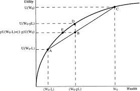
To understand the consequences of paying benefits only to those who are not working, let us suppose that a workers’ compensation program is structured so that, after injury, workers receive their pre-injury earnings for as long as they are off work. Once they work even one hour, however, they are no longer considered disabled and cannot receive further benefits. The effects of this program on work incentives are analyzed in Figure 6.13, in which it is assumed that the pre-injury budget constraint was $A B$ and preinjury earnings were $E_0(=A C$ ). Furthermore, we assume that the worker’s “market” budget constraint (that is, the constraint in the absence of a workers’ compensation program) is unchanged, so that after recovery, the pre-injury wage can again be earned. Under these conditions, the post-injury budget constraint is $B A C$, and the person maximizes utility at point $C$-a point of no work.

Note that constraint $B A C$ contains the segment $A C$, which looks like a spike. It is this spike that creates severe work-incentive problems, for two reasons. First, the returns associated with the first hour of work are negative. That is, a person at point $C$ who returns to work for 1 hour would find his or her income to be considerably reduced by working. Earnings from this hour of work would be more than offset by the reduction in benefits, which creates a negative “net wage.” The substitution effect associated with this program characteristic clearly discourages work. $\frac{20}{}$

Second, our assumed no-work benefit of $A C$ is equal to $E_0$, the preinjury level of earnings. If the worker values leisure at all (as is assumed by the standard downward slope of indifference curves), being able to receive the old level of earnings while also enjoying more leisure clearly enhances utility. The worker is better off at point $C$ than at point $f$, the pre-injury combination of earnings and leisure hours, because he or she is on indifference curve $U_2$ rather than $U_1$. Allowing workers to reach a higher utility level without working generates an income effect that discourages, or at least slows, the return to work.

Indeed, the program we have assumed raises a worker’s reservation wage above his or her pre-injury wage, meaning that a return to work is possible only if the worker qualifies for a higher-paying job. To see this graphically, observe the dashed blue line in Figure 6.13 that begins at point $A$ and is tangent to indifference curve $U_2$ (the level of utility made possible by the social insurance program). The slope of this line is equal to the person’s reservation wage, because if the person can obtain the desired hours of work at this or a greater wage, utility will be at least equal to that associated with point $C$. Note also that for labor force participation to be induced, the reservation wage must be received for at least $R^{\star}$ hours of work.

经济代写|劳动经济学代写Labor Economics代考|Programs with Net Wage Rates of Zero

The programs just discussed were intended to confer benefits on those who are unable to work, and the budget-constraint spike was created by the eligibility requirement that to receive benefits, one must not be working. Other social programs, such as welfare, have different eligibility criteria and calculate benefits differently. These programs factor income needs into their eligibility criteria and then pay benefits based on the difference between one’s actual earnings and one’s needs. We will see that paying people the difference between their earnings and their needs creates a net wage rate of zero; thus, the work-incentive problems associated with these welfare programs result from the fact that they increase the income of program recipients while also drastically reducing the price of leisure.

Nature of Welfare Subsidies Originally, welfare programs tended to take the form of a guaranteed annual income, under which the welfare agency determined the income needed by an eligible person $\left(Y_n\right.$ in Figure 6.14) based on family size, area living costs, and local welfare regulations. Actual earnings were then subtracted from this needed level, and a check was issued to the person each month for the difference. If the person did not work, he or she received a subsidy of $Y_n$. If the person worked, and if earnings caused dollar-for-dollar reductions in welfare benefits, then a budget constraint like $A B C D$ in Figure 6.14 was created. The person’s income remained at $Y_n$ as long as he or she was subsidized. If receiving the subsidy, then, an extra hour of work yielded no net increase in income, because the extra earnings resulted in an equal reduction in welfare benefits. The net wage of a person on the program-and therefore his or her price of leisure-was zero, which is graphically shown by the segment of the constraint having a slope of zero $(B C) .^{22}$

Thus, a welfare program like the one summarized in Figure 6.14 increases the income of the poor by moving the lower end of the budget constraint out from $A C$ to $A B C$; as indicated by the dashed hypothetical constraint in Figure 6.14, this shift creates an income effect tending to reduce labor supply from the hours associated with point $E$ to those associated with point $F$. However, it also causes the wage to effectively drop to zero; every dollar earned is matched by a dollar reduction in welfare benefits. This dollar-for-dollar reduction in benefits induces a huge substitution effect, causing those accepting welfare to reduce their hours of work to zero (point B). Of course, if a person’s indifference curves were sufficiently flat so that the curve tangent to segment $C D$ passed above point $B$ (see Figure 6.15), then that person’s utility would be maximized by choosing work instead of welfare. .23

劳动经济学代考

经济代写|劳动经济学代写Labor Economics代考|Budget Constraints with “Spikes”

一些社会保险计划补偿因临时工伤、永久性残疾或裁员而无法工作的工人。工人赔偿保险可以弥补工人在工作中受伤时的大部分收入损失，私人或公共残疾计划也可以为因其他原因在身体或情感上无法工作的工人提供同样的服务。失业补偿金支付给那些失去工作且无法找到另一份工作的人。虽然在偶尔的司法管辖区可以找到例外情况，19一般来说，这些收入替代计划确实有一个共同特点：它们只向没有工作的人支付福利。

为了理解只向不工作的人支付福利的后果，让我们假设工人赔偿计划的结构是这样的，即工伤发生后，只要他们下班，工人们就可以获得工伤前的收入。然而，一旦他们工作了一个小时，他们就不再被视为残疾并且无法获得进一步的福利。图 6.13 分析了该计划对工作激励的影响，其中假设受伤前预算约束为A乙受伤前的收入是和0(=AC). 此外，我们假设工人的“市场”预算约束（即没有工人补偿计划时的约束）不变，因此在恢复后，可以再次赚取受伤前的工资。在这些条件下，受伤后预算约束为乙AC，并且这个人在点最大化效用C- 一个没有工作的地方。

注意约束乙AC包含段AC，看起来像一个尖峰。正是这种激增造成了严重的工作激励问题，原因有二。首先，与第一个小时工作相关的回报是负的。也就是说，一个人在点C返回工作 1 小时的人会发现他或她的收入因工作而大大减少。这一小时的工作收入将被福利的减少所抵消，从而产生负的“净工资”。与此程序特征相关的替代效应显然会阻碍工作。20

其次，我们假设的无工作收益AC等于和0, 受伤前的收入水平。如果工人完全重视闲暇（正如无差异曲线的标准向下斜率所假设的那样），那么能够在获得原来水平的收入的同时享受更多的闲暇显然会提高效用。工人在这一点上过得更好C比点F，受伤前收入和休闲时间的组合，因为他或她处于无差异曲线上在2而不是在1. 允许工人在不工作的情况下达到更高的效用水平会产生收入效应，从而阻碍或至少减缓重返工作岗位。

事实上，我们假设的计划将工人的保留工资提高到高于他或她受伤前的工资，这意味着只有当工人有资格获得更高薪水的工作时，才有可能重返工作岗位。要以图形方式查看这一点，请观察图 6.13 中从点开始的蓝色虚线A并且与无差异曲线相切在2（社会保险计划使效用水平成为可能）。这条线的斜率等于这个人的保留工资，因为如果这个人能以这个或更高的工资获得想要的工作时间，效用将至少等于与点相关的效用C. 另请注意，要诱导劳动力参与，必须至少收到保留工资R⋆几小时的工作。

经济代写|劳动经济学代写Labor Economics代考|Programs with Net Wage Rates of Zero

刚刚讨论的计划旨在为那些无法工作的人提供福利，而预算限制激增是由资格要求造成的，即必须不工作才能获得福利。其他社会计划，如福利，有不同的资格标准并以不同方式计算福利。这些计划将收入需求纳入其资格标准，然后根据个人实际收入与需求之间的差异支付福利。我们将看到，支付人们收入与需求之间的差额会导致净工资率为零；因此，与这些福利计划相关的工作激励问题是因为它们增加了计划接受者的收入，同时也大大降低了休闲的价格。

福利补贴的性质 最初，福利计划倾向于采取保证年收入的形式，在这种形式下，福利机构确定符合条件的人所需的收入(和n在图 6.14 中）基于家庭规模、地区生活成本和地方福利法规。然后从这个所需水平中减去实际收入，每个月都会向该人开出一张支票以弥补差额。如果此人不工作，他或她将获得补贴和n. 如果这个人工作了，如果收入导致福利减少一美元对一美元，那么预算约束就像A乙C丁在图 6.14 中创建。该人的收入保持在和n只要他或她得到补贴。如果得到补贴，那么，额外工作一个小时不会产生收入的净增加，因为额外的收入导致福利福利的减少。一个人在该计划中的净工资——因此他或她的闲暇价格——为零，这由斜率为零的约束部分以图形方式显示(乙C).22

因此，如图 6.14 中总结的福利计划通过将预算约束线的下端移出AC到A乙C; 如图 6.14 中的虚线假设约束所示，这种转变产生了一种收入效应，倾向于减少与点相关的劳动力供应和与点相关的人F. 然而，这也导致工资实际上降为零；每赚一美元，福利金就会减少一美元。这种逐美元减少的福利会产生巨大的替代效应，导致那些接受福利的人将他们的工作时间减少到零（B 点）。当然，如果一个人的无差异曲线足够平坦以至于曲线与线段相切C丁通过以上点乙（见图 6.15），那么这个人的效用将通过选择工作而不是福利来最大化。.23

统计代写请认准statistics-lab™. statistics-lab™为您的留学生涯保驾护航。

金融工程代写

金融工程是使用数学技术来解决金融问题。金融工程使用计算机科学、统计学、经济学和应用数学领域的工具和知识来解决当前的金融问题，以及设计新的和创新的金融产品。

非参数统计代写

非参数统计指的是一种统计方法，其中不假设数据来自于由少数参数决定的规定模型；这种模型的例子包括正态分布模型和线性回归模型。

广义线性模型代考

广义线性模型（GLM）归属统计学领域，是一种应用灵活的线性回归模型。该模型允许因变量的偏差分布有除了正态分布之外的其它分布。

术语 广义线性模型（GLM）通常是指给定连续和/或分类预测因素的连续响应变量的常规线性回归模型。它包括多元线性回归，以及方差分析和方差分析（仅含固定效应）。

有限元方法代写

有限元方法（FEM）是一种流行的方法，用于数值解决工程和数学建模中出现的微分方程。典型的问题领域包括结构分析、传热、流体流动、质量运输和电磁势等传统领域。

有限元是一种通用的数值方法，用于解决两个或三个空间变量的偏微分方程（即一些边界值问题）。为了解决一个问题，有限元将一个大系统细分为更小、更简单的部分，称为有限元。这是通过在空间维度上的特定空间离散化来实现的，它是通过构建对象的网格来实现的：用于求解的数值域，它有有限数量的点。边界值问题的有限元方法表述最终导致一个代数方程组。该方法在域上对未知函数进行逼近。[1] 然后将模拟这些有限元的简单方程组合成一个更大的方程系统，以模拟整个问题。然后，有限元通过变化微积分使相关的误差函数最小化来逼近一个解决方案。

tatistics-lab作为专业的留学生服务机构，多年来已为美国、英国、加拿大、澳洲等留学热门地的学生提供专业的学术服务，包括但不限于Essay代写，Assignment代写，Dissertation代写，Report代写，小组作业代写，Proposal代写，Paper代写，Presentation代写，计算机作业代写，论文修改和润色，网课代做，exam代考等等。写作范围涵盖高中，本科，研究生等海外留学全阶段，辐射金融，经济学，会计学，审计学，管理学等全球99%专业科目。写作团队既有专业英语母语作者，也有海外名校硕博留学生，每位写作老师都拥有过硬的语言能力，专业的学科背景和学术写作经验。我们承诺100%原创，100%专业，100%准时，100%满意。

随机分析代写

随机微积分是数学的一个分支，对随机过程进行操作。它允许为随机过程的积分定义一个关于随机过程的一致的积分理论。这个领域是由日本数学家伊藤清在第二次世界大战期间创建并开始的。

时间序列分析代写

随机过程，是依赖于参数的一组随机变量的全体，参数通常是时间。 随机变量是随机现象的数量表现，其时间序列是一组按照时间发生先后顺序进行排列的数据点序列。通常一组时间序列的时间间隔为一恒定值（如1秒，5分钟，12小时，7天，1年），因此时间序列可以作为离散时间数据进行分析处理。研究时间序列数据的意义在于现实中，往往需要研究某个事物其随时间发展变化的规律。这就需要通过研究该事物过去发展的历史记录，以得到其自身发展的规律。

回归分析代写

多元回归分析渐进（Multiple Regression Analysis Asymptotics）属于计量经济学领域，主要是一种数学上的统计分析方法，可以分析复杂情况下各影响因素的数学关系，在自然科学、社会和经济学等多个领域内应用广泛。

MATLAB代写

MATLAB 是一种用于技术计算的高性能语言。它将计算、可视化和编程集成在一个易于使用的环境中，其中问题和解决方案以熟悉的数学符号表示。典型用途包括：数学和计算算法开发建模、仿真和原型制作数据分析、探索和可视化科学和工程图形应用程序开发，包括图形用户界面构建MATLAB 是一个交互式系统，其基本数据元素是一个不需要维度的数组。这使您可以解决许多技术计算问题，尤其是那些具有矩阵和向量公式的问题，而只需用 C 或 Fortran 等标量非交互式语言编写程序所需的时间的一小部分。MATLAB 名称代表矩阵实验室。MATLAB 最初的编写目的是提供对由 LINPACK 和 EISPACK 项目开发的矩阵软件的轻松访问，这两个项目共同代表了矩阵计算软件的最新技术。MATLAB 经过多年的发展，得到了许多用户的投入。在大学环境中，它是数学、工程和科学入门和高级课程的标准教学工具。在工业领域，MATLAB 是高效研究、开发和分析的首选工具。MATLAB 具有一系列称为工具箱的特定于应用程序的解决方案。对于大多数 MATLAB 用户来说非常重要，工具箱允许您学习和应用专业技术。工具箱是 MATLAB 函数（M 文件）的综合集合，可扩展 MATLAB 环境以解决特定类别的问题。可用工具箱的领域包括信号处理、控制系统、神经网络、模糊逻辑、小波、仿真等。

R语言代写	问卷设计与分析代写
PYTHON代写	回归分析与线性模型代写
MATLAB代写	方差分析与试验设计代写
STATA代写	机器学习/统计学习代写
SPSS代写	计量经济学代写
EVIEWS代写	时间序列分析代写
EXCEL代写	深度学习代写
SQL代写	各种数据建模与可视化代写

如果你也在 怎样代写劳动经济学Labor Economics这个学科遇到相关的难题，请随时右上角联系我们的24/7代写客服。

劳动经济学，或称劳工经济学，旨在了解雇佣劳动市场的运作和动态。劳动是一种商品，由劳动者提供，通常是为了换取有要求的公司支付的工资。

statistics-lab™ 为您的留学生涯保驾护航 在代写劳动经济学Labor Economics方面已经树立了自己的口碑, 保证靠谱, 高质且原创的统计Statistics代写服务。我们的专家在代写劳动经济学Labor Economics代写方面经验极为丰富，各种代写劳动经济学Labor Economics相关的作业也就用不着说。

我们提供的劳动经济学Labor Economics及其相关学科的代写，服务范围广, 其中包括但不限于:

• Statistical Inference 统计推断
• Statistical Computing 统计计算
• Advanced Probability Theory 高等概率论
• Advanced Mathematical Statistics 高等数理统计学
• (Generalized) Linear Models 广义线性模型
• Statistical Machine Learning 统计机器学习
• Longitudinal Data Analysis 纵向数据分析
• Foundations of Data Science 数据科学基础

经济代写|劳动经济学代写Labor Economics代考|Analysis of the Labor/Leisure Choice

This section introduces indifference curves and budget constraints-visual aids that make the theory of labor supply easier to understand and to apply to complex policy issues. These graphical aids visually depict the basic factors underlying the demand for leisure (supply of labor) discussed earlier.

Preferences Let us assume that there are two major categories of goods that make people happy-leisure time and the goods people can buy with money. If we take the prices of goods as fixed, then they can be compressed into one index that is measured by money income (with prices fixed, more money income means it is possible to consume more goods). Using two categories, leisure and money income, allows our graphs to be drawn in two-dimensional space.

Since both leisure and money can be used to generate satisfaction (or utility), these two goods are to some extent substitutes for each other. If forced to give up some money income-by cutting back on hours of work, for example-some increase in leisure time could be substituted for this lost income to keep a person as happy as before.
To understand how preferences can be graphed, suppose a thoughtful consumer/worker were asked to decide how happy he or she would be with a daily income of $\$ 64$ combined with 8 hours of leisure (point $a$ in Figure 6.2). This level of happiness could be called utility level $A$. Our consumer/worker could name other combinations of money income and leisure hours that would also yield utility level $A$. Assume that our respondent named five other combinations. All six combinations of money income and leisure hours that yield utility level $A$ are represented by heavy dots in Figure 6.2. The curve connecting these dots is called an indifference curve, which connects the various combinations of money income and leisure that yield equal utility. (The term indifference curve is derived from the fact that since each point on the curve yields equal utility, a person is truly indifferent about where on the curve he or she will be.)

经济代写|劳动经济学代写Labor Economics代考|Empirical Findings on the Income and Substitution Effects

Labor supply theory suggests that the choices workers make concerning their desired hours of work depend on their wealth and the wage rate they can command, in addition to their preferences. In particular, this theory suggests the existence of a negative income effect and a positive substitution effect. Empirical tests of labor supply theory generally attempt to determine if these two effects can be observed, if they operate in the expected directions, and what their relative magnitudes are.

Most recent studies of labor supply have used large samples of individuals to analyze how labor force participation and hours of work are affected by changes in wage rates and income-often induced by changes in taxes- holding other influences (age, for example) constant. Studies of male and female labor force behavior are done separately because of the different roles men and women typically play in performing household work and child-rearing-activities that clearly affect labor supply decisions but about which information is usually very limited.

A comprehensive review of numerous studies of the labor supply behavior of men finds that the sizes of the estimated effects vary with both the data and the statistical methodology used. Taken as a whole, however, the studies find strong evidence that, as theory suggests, observed substitution effects are positive and observed income effects are negative. What is less clear is which effect dominates when wages change; indeed, it appears that the typical study finds the two effects to be roughly similar in magnitude. $\frac{16}{1}$ Studies of the retirement behavior of older men (a topic we will address in chapter 7 ) find, also as theory suggests, that the substitution effect dominates the decision to withdraw from the labor force. $\frac{17}{}$

Studies of the labor supply behavior of women generally have found a greater responsiveness to wage changes than is found among men. As noted earlier, labor supply can be measured both by labor force participation rates and by hours of work.

Historically, women’s labor force participation rates have been more responsive than men’s to wage changes. (As seen in Fxample 6.4, the lahor force participation rate for married women has also been more responsive to wage changes than have been their hours of work.) There is evidence, however, that in the last two decades, the labor supply behavior of women has become much more similar to that for men-meaning that the labor supply of women is becoming less responsive to wage changes than it used to be. The reduced responsiveness has been especially noticeable in women’s labor force participation decisions, where the differences between men and women have been similarity in the expectations held by women and men concerning work and careers.

劳动经济学代考

经济代写|劳动经济学代写Labor Economics代考|Analysis of the Labor/Leisure Choice

本节介绍无差异曲线和预算约束——使劳动力供给理论更易于理解和应用于复杂政策问题的视觉辅助工具。这些图形辅助工具直观地描述了前面讨论的休闲需求（劳动力供应）背后的基本因素。

偏好 让我们假设有两大类使人们快乐的商品——休闲时间和人们可以用金钱购买的商品。如果我们把商品的价格看成是固定的，那么就可以把它们压缩成一个用货币收入来衡量的指标（价格固定，货币收入多，就可以消费更多的商品）。使用两个类别，休闲和金钱收入，允许我们在二维空间中绘制图表。

由于闲暇和金钱都可以用来产生满足感（或效用），这两种商品在某种程度上可以相互替代。如果被迫放弃一些货币收入——例如，通过减少工作时间——可以增加一些闲暇时间来弥补失去的收入，使一个人像以前一样快乐。
为了理解偏好是如何被绘制出来的，假设一位有思想的消费者/工人被要求决定他或她对每天收入为$64结合 8 小时的休闲（点A在图 6.2 中）。这种幸福水平可以称为效用水平A. 我们的消费者/工人可以说出其他也会产生效用水平的货币收入和闲暇时间的组合A. 假设我们的受访者命名了其他五个组合。产生效用水平的货币收入和闲暇时间的所有六种组合A在图 6.2 中用粗点表示。连接这些点的曲线称为无差异曲线，它连接产生相等效用的货币收入和闲暇的各种组合。（术语“无差异曲线”源于这样一个事实，即由于曲线上的每个点都产生相等的效用，因此一个人对他或她将在曲线上的哪个位置真正无关紧要。）

经济代写|劳动经济学代写Labor Economics代考|Empirical Findings on the Income and Substitution Effects

劳动力供给理论表明，工人对他们期望的工作时间做出的选择除了他们的偏好外，还取决于他们的财富和他们可以要求的工资率。特别是，该理论表明存在负收入效应和正替代效应。劳动力供给理论的实证检验通常试图确定这两种效应是否可以观察到，它们是否在预期的方向上运作，以及它们的相对大小是多少。

大多数最近的劳动力供应研究都使用了大量的个人样本来分析劳动力参与和工作时间如何受到工资率和收入变化的影响——通常是由税收变化引起的——保持其他影响（例如年龄）不变。男性和女性劳动力行为的研究是分开进行的，因为男性和女性通常在家务劳动和育儿活动中扮演不同的角色，这些活动显然会影响劳动力供应决策，但相关信息通常非常有限。

对男性劳动力供应行为的大量研究进行全面审查后发现，估计影响的大小因所使用的数据和统计方法而异。然而，从整体上看，研究发现强有力的证据表明，正如理论所表明的那样，观察到的替代效应是积极的，而观察到的收入影响是消极的。不太清楚的是，当工资发生变化时，哪种效应占主导地位？事实上，典型的研究似乎发现这两种影响的幅度大致相似。161对老年男性退休行为（我们将在第 7 章讨论的主题）的研究发现，也正如理论所表明的那样，替代效应支配着退出劳动力的决定。17

对女性劳动力供给行为的研究普遍发现，女性对工资变化的反应比男性更强。如前所述，劳动力供应可以通过劳动力参与率和工作时间来衡量。

从历史上看，女性的劳动力参与率比男性对工资变化的反应更为敏感。（如示例 6.4 所示，已婚妇女的劳动力参与率对工资变化的反应也比对工作时间的反应更敏感。）然而，有证据表明，在过去的二十年中，已婚妇女的劳动力供给行为女性变得与男性更加相似——这意味着女性的劳动力供应对工资变化的反应不如过去。在女性劳动力参与决策中，响应性的降低尤为明显，男性和女性之间的差异在女性和男性对工作和职业的期望方面存在相似之处。

统计代写请认准statistics-lab™. statistics-lab™为您的留学生涯保驾护航。

金融工程代写

金融工程是使用数学技术来解决金融问题。金融工程使用计算机科学、统计学、经济学和应用数学领域的工具和知识来解决当前的金融问题，以及设计新的和创新的金融产品。

非参数统计代写

非参数统计指的是一种统计方法，其中不假设数据来自于由少数参数决定的规定模型；这种模型的例子包括正态分布模型和线性回归模型。

广义线性模型代考

广义线性模型（GLM）归属统计学领域，是一种应用灵活的线性回归模型。该模型允许因变量的偏差分布有除了正态分布之外的其它分布。

术语 广义线性模型（GLM）通常是指给定连续和/或分类预测因素的连续响应变量的常规线性回归模型。它包括多元线性回归，以及方差分析和方差分析（仅含固定效应）。

有限元方法代写

有限元方法（FEM）是一种流行的方法，用于数值解决工程和数学建模中出现的微分方程。典型的问题领域包括结构分析、传热、流体流动、质量运输和电磁势等传统领域。

有限元是一种通用的数值方法，用于解决两个或三个空间变量的偏微分方程（即一些边界值问题）。为了解决一个问题，有限元将一个大系统细分为更小、更简单的部分，称为有限元。这是通过在空间维度上的特定空间离散化来实现的，它是通过构建对象的网格来实现的：用于求解的数值域，它有有限数量的点。边界值问题的有限元方法表述最终导致一个代数方程组。该方法在域上对未知函数进行逼近。[1] 然后将模拟这些有限元的简单方程组合成一个更大的方程系统，以模拟整个问题。然后，有限元通过变化微积分使相关的误差函数最小化来逼近一个解决方案。

tatistics-lab作为专业的留学生服务机构，多年来已为美国、英国、加拿大、澳洲等留学热门地的学生提供专业的学术服务，包括但不限于Essay代写，Assignment代写，Dissertation代写，Report代写，小组作业代写，Proposal代写，Paper代写，Presentation代写，计算机作业代写，论文修改和润色，网课代做，exam代考等等。写作范围涵盖高中，本科，研究生等海外留学全阶段，辐射金融，经济学，会计学，审计学，管理学等全球99%专业科目。写作团队既有专业英语母语作者，也有海外名校硕博留学生，每位写作老师都拥有过硬的语言能力，专业的学科背景和学术写作经验。我们承诺100%原创，100%专业，100%准时，100%满意。

随机分析代写

随机微积分是数学的一个分支，对随机过程进行操作。它允许为随机过程的积分定义一个关于随机过程的一致的积分理论。这个领域是由日本数学家伊藤清在第二次世界大战期间创建并开始的。

时间序列分析代写

随机过程，是依赖于参数的一组随机变量的全体，参数通常是时间。 随机变量是随机现象的数量表现，其时间序列是一组按照时间发生先后顺序进行排列的数据点序列。通常一组时间序列的时间间隔为一恒定值（如1秒，5分钟，12小时，7天，1年），因此时间序列可以作为离散时间数据进行分析处理。研究时间序列数据的意义在于现实中，往往需要研究某个事物其随时间发展变化的规律。这就需要通过研究该事物过去发展的历史记录，以得到其自身发展的规律。

回归分析代写

多元回归分析渐进（Multiple Regression Analysis Asymptotics）属于计量经济学领域，主要是一种数学上的统计分析方法，可以分析复杂情况下各影响因素的数学关系，在自然科学、社会和经济学等多个领域内应用广泛。

MATLAB代写

MATLAB 是一种用于技术计算的高性能语言。它将计算、可视化和编程集成在一个易于使用的环境中，其中问题和解决方案以熟悉的数学符号表示。典型用途包括：数学和计算算法开发建模、仿真和原型制作数据分析、探索和可视化科学和工程图形应用程序开发，包括图形用户界面构建MATLAB 是一个交互式系统，其基本数据元素是一个不需要维度的数组。这使您可以解决许多技术计算问题，尤其是那些具有矩阵和向量公式的问题，而只需用 C 或 Fortran 等标量非交互式语言编写程序所需的时间的一小部分。MATLAB 名称代表矩阵实验室。MATLAB 最初的编写目的是提供对由 LINPACK 和 EISPACK 项目开发的矩阵软件的轻松访问，这两个项目共同代表了矩阵计算软件的最新技术。MATLAB 经过多年的发展，得到了许多用户的投入。在大学环境中，它是数学、工程和科学入门和高级课程的标准教学工具。在工业领域，MATLAB 是高效研究、开发和分析的首选工具。MATLAB 具有一系列称为工具箱的特定于应用程序的解决方案。对于大多数 MATLAB 用户来说非常重要，工具箱允许您学习和应用专业技术。工具箱是 MATLAB 函数（M 文件）的综合集合，可扩展 MATLAB 环境以解决特定类别的问题。可用工具箱的领域包括信号处理、控制系统、神经网络、模糊逻辑、小波、仿真等。

R语言代写	问卷设计与分析代写
PYTHON代写	回归分析与线性模型代写
MATLAB代写	方差分析与试验设计代写
STATA代写	机器学习/统计学习代写
SPSS代写	计量经济学代写
EVIEWS代写	时间序列分析代写
EXCEL代写	深度学习代写
SQL代写	各种数据建模与可视化代写

如果你也在 怎样代写劳动经济学Labor Economics这个学科遇到相关的难题，请随时右上角联系我们的24/7代写客服。

劳动经济学，或称劳工经济学，旨在了解雇佣劳动市场的运作和动态。劳动是一种商品，由劳动者提供，通常是为了换取有要求的公司支付的工资。

statistics-lab™ 为您的留学生涯保驾护航 在代写劳动经济学Labor Economics方面已经树立了自己的口碑, 保证靠谱, 高质且原创的统计Statistics代写服务。我们的专家在代写劳动经济学Labor Economics代写方面经验极为丰富，各种代写劳动经济学Labor Economics相关的作业也就用不着说。

我们提供的劳动经济学Labor Economics及其相关学科的代写，服务范围广, 其中包括但不限于:

• Statistical Inference 统计推断
• Statistical Computing 统计计算
• Advanced Probability Theory 高等概率论
• Advanced Mathematical Statistics 高等数理统计学
• (Generalized) Linear Models 广义线性模型
• Statistical Machine Learning 统计机器学习
• Longitudinal Data Analysis 纵向数据分析
• Foundations of Data Science 数据科学基础

经济代写|劳动经济学代写Labor Economics代考|Can the Laws of Derived Demand Be Applied to Cross-Elasticities?

The Hicks-Marshall laws of derived demand are based on four technological or market conditions that determine the size of own-wage elasticities. Each of the four conditions influences the substitution or the scale effect, and as noted above, the relative strengths of these two effects are also what determine the sign of cross-elasticities. The laws that apply to own-wage elasticities cannot be applied directly to cross-elasticities because with cross-elasticities, the substitution effect (if there is one) and the scale effect work in opposite directions. The same underlying considerations, however, are basic to an analysis of cross-elasticities.

As we discuss these four considerations in the context of cross-elasticities, it will be helpful to have an example in mind. Let us return, then, to the question of what might happen to the demand for adult workers if the wages of teenage workers were to fall. As noted above, the answer depends on the relative strengths of the scale and substitution effects. What determines the strength of each?

The Scale Effect The most immediate effect of a fall in the wages of teenagers would be reduced production costs for those firms that employ them. Competition in the product market would ensure that lower costs are followed by price reductions, which should stimulate increases in both product demand and the level of output. Increased levels of output will tend to cause increases in employment of all kinds of workers, including adults. This chain of events obviously describes behavior underlying the scale effect, and we now investigate what conditions are likely to make for a strong (or weak) scale effect.
The initial cost (and price) reductions would be greater among those employers for whom teenage wages constituted a higher proportion of total costs. Other things equal, greater price reductions would result in greater increases in both product demand and overall employment. Thus, the share of total costs devoted to the productive factor whose price is changing will influence the size of the scale effect. The larger this share, other things equal, the greater the scale effect (and the more likely it is that gross complementarity will exist). This tendency is analogous to the fourth Hicks-Marshall law discussed earlier; the difference is that with cross-elasticities, the factor whose price is changing is not the same as the one for which employment changes are being analyzed.
The other condition that greatly influences the size of the scale effect is product demand elasticity. In the earlier case of teenage wage reductions, the greater the increase in product demand when firms reduce their prices, the greater the tendency for employment of all workers, including adults, to increase. More generally, the greater the price elasticity of product demand, other things equal, the greater the scale effect (and thus the greater the likelihood of gross complementarity). The effects of product demand elasticity are thus similar for both own-wage and cross-wage elasticities.

经济代写|劳动经济学代写Labor Economics代考|Estimates Relating to Cross-Elasticities

Estimating at least the sign of cross-wage labor demand elasticities is useful for answering many public-policy questions. For example, if we were to reduce the teenage minimum wage, how would this affect the demand for adult labor? If capital were to be subsidized, how would this affect the demand for labor? Or, to take a hotly debated issue in recent years (and one we will return to in chapter 10), when immigrant labor becomes cheaper and more available, what are the likely effects on the demand for various grades of native labor? These questions, of course, are really asking whether the pairs of inputs italicized in each sentence are gross complements or gross substitutes.

While the major policy interest is whether two inputs are gross complements or gross substitutes, obtaining credible estimates is challenging (because it is difficult to estimate scale effects). Therefore, most of the cross-wage empirical studies to date focus on whether two factors are substitutes or complements in production. These studies estimate the employment response for one category of labor to a wage or price change elsewhere, holding output constant (which in effect allows us to focus just on changes in the mix of factors used in production). The factors of production paired together for analysis in these studies are numerous, and the results are not always clear-cut; nevertheless, the findings taken as a whole offer at least a few generalizations: $\frac{10}{}$

1. Labor and energy are clearly substitutes in production, although their degree of substitutability is small. Labor and materials are probably substitutes in production, with the degree of substitutability again being small.
2. Skilled labor and unskilled labor are substitutes in production. 11
3. We are not certain whether either skilled or unskilled labor is a substitute for or a complement with capital in the production process. What does appear to be true is that skilled (or well-educated) labor is more likely to be complementary with capital than is unskilled labor-and that if they are both substitutes for capital, the degree of substitutability is smaller for skilled labor: $12$
4. The finding summarized in 3 above suggests that skilled labor is more likely than unskilled labor to be a gross complement with capital. This finding is important to our understanding of recent trends in the earnings of skilled and unskilled workers (see chapter 15 ), because the prices of computers and other high-tech capital goods have fallen dramatically in the past decade or so.

劳动经济学代考

经济代写|劳动经济学代写劳动经济学代考|派生需求定律可以应用于交叉弹性吗?

派生需求的希克斯-马歇尔定律基于四种技术或市场条件，这些条件决定了自身工资弹性的大小。这四种条件中的每一种都会影响替代效应或尺度效应，如上所述，这两种效应的相对强度也决定了交叉弹性的符号。适用于自身工资弹性的定律不能直接适用于交叉弹性，因为在交叉弹性中，替代效应(如果存在的话)和规模效应的作用方向是相反的。然而，同样的潜在考虑也是交叉弹性分析的基础

当我们在交叉弹性的背景下讨论这四个考虑因素时，脑海中有一个例子将是有帮助的。那么，让我们回到这个问题上来:如果青少年工人的工资下降，对成年工人的需求会发生什么变化?如上所述，答案取决于规模和替代效应的相对强度。是什么决定了它们的力量?

规模效应青少年工资下降最直接的影响将是雇佣他们的公司的生产成本降低。产品市场的竞争将确保在降低成本之后会有价格的降低，这将刺激产品需求和产出水平的增加。产出水平的提高将导致包括成年人在内的各类工人的就业增加。这个事件链显然描述了规模效应下的行为，我们现在研究什么条件可能会产生强(或弱)的规模效应。对于那些青少年工资在总成本中所占比例较高的雇主来说，初始成本(和价格)的削减将更大。在其他条件相同的情况下，更大幅度的降价将导致产品需求和整体就业的更大增长。因此，价格变化的生产要素在总成本中所占的份额将影响规模效应的大小。在其他条件相同的情况下，这一份额越大，规模效应就越大(总体互补就越有可能存在)。这种趋势类似于前面讨论的希克斯-马歇尔第四定律;不同的是，在交叉弹性中，价格变化的因素与就业变化被分析的因素是不同的。另一个对规模效应大小有很大影响的条件是产品需求弹性。在早期的青少年减薪案例中，当公司降低价格时，产品需求的增长越大，所有工人(包括成年人)的就业增长趋势就越大。更一般地说，在其他条件相同的情况下，产品需求的价格弹性越大，规模效应就越大(因此总互补性的可能性就越大)。因此，产品需求弹性对自身工资弹性和跨工资弹性的影响是相似的

经济代写|劳动经济学代写劳动经济学代考|有关交叉弹性的估计

至少估计跨工资劳动需求弹性的迹象对于回答许多公共政策问题是有用的。例如，如果我们降低青少年的最低工资，这将如何影响对成人劳动力的需求?如果资本得到补贴，这将如何影响对劳动力的需求?或者，以近年来一个激烈争论的问题为例(我们将在第十章中再次讨论这个问题)，当移民劳动力变得更便宜、更容易获得时，对不同等级本地劳动力的需求可能会产生什么影响?当然，这些问题实际上是在问每句中斜体显示的输入对是总的补充还是总的替代

虽然主要政策关注的是两项投入是总的补充还是总的替代，但获得可靠的估计数是具有挑战性的(因为很难估计规模效应)。因此，迄今为止的跨工资实证研究大多关注两个因素在生产中是替代还是互补。这些研究在保持产出不变的情况下，估计了某一类劳动力对其他领域工资或价格变化的就业反应(这实际上使我们能够只关注生产中使用的各种因素的组合变化)。在这些研究中，成对进行分析的生产因素有很多，结果并不总是明确的;尽管如此，作为一个整体，这些发现至少提供了一些概括:$\frac{10}{}$

劳动和能源在生产中显然是替代品，尽管它们的可替代性程度很小。劳动力和材料在生产中很可能是替代品，可替代性的程度也很小。熟练工人和非熟练工人是生产中的替代品。我们不能肯定在生产过程中，技术劳动和非技术劳动是资本的替代品还是补充。似乎是正确的是，技术劳动(或受过良好教育的)与非技术劳动相比更有可能与资本互补，而且如果它们都是资本的替代品，那么对技术劳动的可替代程度就更小:$12$以上3中总结的发现表明，技术劳动比非技术劳动更有可能是资本的总补充。这一发现对于我们理解技术工人和非技术工人的收入的最近趋势是很重要的(见第15章)，因为计算机和其他高科技资本货物的价格在过去十多年来急剧下降

统计代写请认准statistics-lab™. statistics-lab™为您的留学生涯保驾护航。

金融工程代写

金融工程是使用数学技术来解决金融问题。金融工程使用计算机科学、统计学、经济学和应用数学领域的工具和知识来解决当前的金融问题，以及设计新的和创新的金融产品。

非参数统计代写

非参数统计指的是一种统计方法，其中不假设数据来自于由少数参数决定的规定模型；这种模型的例子包括正态分布模型和线性回归模型。

广义线性模型代考

广义线性模型（GLM）归属统计学领域，是一种应用灵活的线性回归模型。该模型允许因变量的偏差分布有除了正态分布之外的其它分布。

术语 广义线性模型（GLM）通常是指给定连续和/或分类预测因素的连续响应变量的常规线性回归模型。它包括多元线性回归，以及方差分析和方差分析（仅含固定效应）。

有限元方法代写

有限元方法（FEM）是一种流行的方法，用于数值解决工程和数学建模中出现的微分方程。典型的问题领域包括结构分析、传热、流体流动、质量运输和电磁势等传统领域。

有限元是一种通用的数值方法，用于解决两个或三个空间变量的偏微分方程（即一些边界值问题）。为了解决一个问题，有限元将一个大系统细分为更小、更简单的部分，称为有限元。这是通过在空间维度上的特定空间离散化来实现的，它是通过构建对象的网格来实现的：用于求解的数值域，它有有限数量的点。边界值问题的有限元方法表述最终导致一个代数方程组。该方法在域上对未知函数进行逼近。[1] 然后将模拟这些有限元的简单方程组合成一个更大的方程系统，以模拟整个问题。然后，有限元通过变化微积分使相关的误差函数最小化来逼近一个解决方案。

tatistics-lab作为专业的留学生服务机构，多年来已为美国、英国、加拿大、澳洲等留学热门地的学生提供专业的学术服务，包括但不限于Essay代写，Assignment代写，Dissertation代写，Report代写，小组作业代写，Proposal代写，Paper代写，Presentation代写，计算机作业代写，论文修改和润色，网课代做，exam代考等等。写作范围涵盖高中，本科，研究生等海外留学全阶段，辐射金融，经济学，会计学，审计学，管理学等全球99%专业科目。写作团队既有专业英语母语作者，也有海外名校硕博留学生，每位写作老师都拥有过硬的语言能力，专业的学科背景和学术写作经验。我们承诺100%原创，100%专业，100%准时，100%满意。

随机分析代写

随机微积分是数学的一个分支，对随机过程进行操作。它允许为随机过程的积分定义一个关于随机过程的一致的积分理论。这个领域是由日本数学家伊藤清在第二次世界大战期间创建并开始的。

时间序列分析代写

随机过程，是依赖于参数的一组随机变量的全体，参数通常是时间。 随机变量是随机现象的数量表现，其时间序列是一组按照时间发生先后顺序进行排列的数据点序列。通常一组时间序列的时间间隔为一恒定值（如1秒，5分钟，12小时，7天，1年），因此时间序列可以作为离散时间数据进行分析处理。研究时间序列数据的意义在于现实中，往往需要研究某个事物其随时间发展变化的规律。这就需要通过研究该事物过去发展的历史记录，以得到其自身发展的规律。

回归分析代写

多元回归分析渐进（Multiple Regression Analysis Asymptotics）属于计量经济学领域，主要是一种数学上的统计分析方法，可以分析复杂情况下各影响因素的数学关系，在自然科学、社会和经济学等多个领域内应用广泛。

MATLAB代写

MATLAB 是一种用于技术计算的高性能语言。它将计算、可视化和编程集成在一个易于使用的环境中，其中问题和解决方案以熟悉的数学符号表示。典型用途包括：数学和计算算法开发建模、仿真和原型制作数据分析、探索和可视化科学和工程图形应用程序开发，包括图形用户界面构建MATLAB 是一个交互式系统，其基本数据元素是一个不需要维度的数组。这使您可以解决许多技术计算问题，尤其是那些具有矩阵和向量公式的问题，而只需用 C 或 Fortran 等标量非交互式语言编写程序所需的时间的一小部分。MATLAB 名称代表矩阵实验室。MATLAB 最初的编写目的是提供对由 LINPACK 和 EISPACK 项目开发的矩阵软件的轻松访问，这两个项目共同代表了矩阵计算软件的最新技术。MATLAB 经过多年的发展，得到了许多用户的投入。在大学环境中，它是数学、工程和科学入门和高级课程的标准教学工具。在工业领域，MATLAB 是高效研究、开发和分析的首选工具。MATLAB 具有一系列称为工具箱的特定于应用程序的解决方案。对于大多数 MATLAB 用户来说非常重要，工具箱允许您学习和应用专业技术。工具箱是 MATLAB 函数（M 文件）的综合集合，可扩展 MATLAB 环境以解决特定类别的问题。可用工具箱的领域包括信号处理、控制系统、神经网络、模糊逻辑、小波、仿真等。

R语言代写	问卷设计与分析代写
PYTHON代写	回归分析与线性模型代写
MATLAB代写	方差分析与试验设计代写
STATA代写	机器学习/统计学习代写
SPSS代写	计量经济学代写
EVIEWS代写	时间序列分析代写
EXCEL代写	深度学习代写
SQL代写	各种数据建模与可视化代写

如果你也在 怎样代写劳动经济学Labor Economics这个学科遇到相关的难题，请随时右上角联系我们的24/7代写客服。

劳动经济学，或称劳工经济学，旨在了解雇佣劳动市场的运作和动态。劳动是一种商品，由劳动者提供，通常是为了换取有要求的公司支付的工资。

statistics-lab™ 为您的留学生涯保驾护航 在代写劳动经济学Labor Economics方面已经树立了自己的口碑, 保证靠谱, 高质且原创的统计Statistics代写服务。我们的专家在代写劳动经济学Labor Economics代写方面经验极为丰富，各种代写劳动经济学Labor Economics相关的作业也就用不着说。

我们提供的劳动经济学Labor Economics及其相关学科的代写，服务范围广, 其中包括但不限于:

• Statistical Inference 统计推断
• Statistical Computing 统计计算
• Advanced Probability Theory 高等概率论
• Advanced Mathematical Statistics 高等数理统计学
• (Generalized) Linear Models 广义线性模型
• Statistical Machine Learning 统计机器学习
• Longitudinal Data Analysis 纵向数据分析
• Foundations of Data Science 数据科学基础

经济代写|劳动经济学代写Labor Economics代考|Applying the Laws of Derived Demand: Inferential Analysis

Because empirical estimates of demand elasticities that may be required for making particular decisions are often lacking, it is frequently necessary to guess what these elasticities are likely to be. In making these guesses, we can apply the laws of derived demand to predict at least relative magnitudes for various types of labor. Consider first the demand for unionized New York City garment workers. As we shall discuss in chapter 13 , because unions are complex organizations, it is not always possible to specify what their goals are. Nevertheless, it is clear that most unions value both wage and employment opportunities for their members. This observation leads to the simple prediction that, other things equal, the more elastic the demand for labor, the smaller the wage gain that a union will succeed in winning for its members. The reason for this prediction is that the more elastic the demand curve, the greater the percentage employment decline associated with any given percentage increase in wages. As a result, we can expect the following:

1. Unions would win larger wage gains for their members in markets with inelastic labor demand curves.
2. Unions would strive to take actions that reduce the wage elasticity of demand for their members’ services.
3. Unions might first seek to organize workers in markets in which labor demand curves are inelastic (because the potential gains to unionization are higher in these markets).

Because of foreign competition, the price elasticity of demand for the clothing produced by New York City garment workers is extremely high. Furthermore, employcrs can easily find other inputs to substitute for these workers-namely, lower-paid nonunion garment workers in the South or in other countries. These facts lead one to predict that the wage elasticity of demand for New York City unionized garment workers is very high. Consequently, union wage demands have historically been moderate. The union has also sought to reduce the elasticity of product demand by supporting policies that reduce foreign competition, and it has pushed for higher federal minimum wages to reduce employers’ incentives to move their plants to the South.

经济代写|劳动经济学代写Labor Economics代考|The Cross-Wage Elasticity of Demand

Because firms may employ several categories of labor and capital, the demand for any one category can be affected by price changes in the others. For example, if the wages of carpenters rose, more people might build brick homes and the demand for masons might increase. An increase in carpenters’ wages might decrease the overall level of home building in the economy, however, which would decrease the demand for plumbers. Finally, changes in the price of capital could increase or decrease the demand for workers in all three trades.

The direction and magnitude of the above effects can be summarized by examining the elasticities of demand for inputs with respect to the prices of other inputs. The elasticity of demand for input $j$ with respect to the price of input $k$ is the percentage change in the demand for input $j$ induced by a 1 percent change in the price of input $k$. If the two inputs are both categories of labor, these cross-wage elasticities of demand are given by
$$
\eta \mathrm{jk}=\% \Delta \mathrm{Ej} \% \Delta \mathrm{Wk} x \quad \text { (4.2) }
$$
and
$$
\eta \mathrm{kj}=\% \Delta \mathrm{Ek} \% \Delta \mathrm{Wj}
$$
where, again, the Greek letter $\eta$ is used to represent the elasticity. If the cross-elasticities are positive (with an increase in the price of one “category” increasing the demand for the other), the two are said to be gross substitutes. If these cross-elasticities are negative (and an increase in the price of one “category” reduces the demand for the other), the two are said to be gross complements (refer back to Figure 3.3).

It is worth reiterating that whether two inputs are gross substitutes or gross complements depends on the relative sizes of the scale and substitution effects. To see this, suppose we assume that adults and teenagers are substitutes in production. A decrease in the teenage wage will thus have opposing effects on adult employment. On the one hand, there is a substitution effect: for a given level of output, employers will now have an incentive to substitute teens for adults in the production process and reduce adult employment. On the other hand, there is a scale effect: a lower teenage wage reduces costs and provides employers with an incentive to increase employment of all inputs, including adults.

劳动经济学代考

经济代写|劳动经济学代写劳动经济学代考|应用派生需求定律:推理分析

.

由于往往缺乏对作出特定决定可能需要的需求弹性的经验估计，因此经常需要猜测这些弹性可能是多少。在进行这些猜测时，我们可以应用派生需求定律来预测各种类型劳动的相对规模。首先考虑一下对加入工会的纽约市制衣工人的需求。正如我们将在第13章中讨论的那样，由于工会是复杂的组织，它并不总是能够具体说明他们的目标是什么。然而，很明显，大多数工会都重视其成员的工资和就业机会。这一观察结果导致了一个简单的预测:在其他条件相同的情况下，劳动力需求的弹性越大，工会为其成员成功赢得的工资增长就越小。这一预测的原因是，需求曲线的弹性越大，与任何给定的工资增长百分比相关的就业下降百分比就越大。因此，我们可以预期以下结果:

在劳动力需求曲线无弹性的市场中，工会将为其成员赢得更大的工资增长。工会将努力采取行动，降低其成员服务需求的工资弹性。工会可能首先寻求在劳动力需求曲线无弹性的市场中组织工人(因为在这些市场中加入工会的潜在收益更高)

由于国外的竞争，纽约市服装工人生产的服装需求的价格弹性非常高。此外，雇主可以很容易地找到替代这些工人的其他投入，即南方或其他国家工资较低的非工会服装工人。这些事实使人们预测，纽约市加入工会的服装工人的需求工资弹性非常高。因此，工会对工资的要求历来都是温和的。该工会还试图通过支持减少外国竞争的政策来降低产品需求的弹性，并推动提高联邦最低工资标准，以减少雇主将工厂迁往南方的动机。

经济代写|劳动经济学代写劳动经济学代考|需求的跨工资弹性

因为公司可能雇用几种类型的劳动力和资本，任何一种类型的需求都可能受到其他类型的价格变化的影响。例如，如果木匠的工资上涨，更多的人可能会建造砖房，对泥瓦匠的需求可能会增加。然而，木匠工资的增加可能会降低经济中房屋建筑的整体水平，这将减少对水管工的需求。最后，资本价格的变化会增加或减少这三个行业对工人的需求

通过考察投入需求相对于其他投入价格的弹性，可以总结上述影响的方向和程度。投入$j$的需求相对于投入$k$的价格的弹性是投入$k$的价格变化1％所引起的对投入$j$的需求变化百分比。如果这两种投入都是劳动类别，这些需求的跨工资弹性由
$$
\eta \mathrm{jk}=\% \Delta \mathrm{Ej} \% \Delta \mathrm{Wk} x \quad \text { (4.2) }
$$
和
$$
\eta \mathrm{kj}=\% \Delta \mathrm{Ek} \% \Delta \mathrm{Wj}
$$
给出，其中，同样，用希腊字母$\eta$表示弹性。如果交叉弹性是正的(一种“类别”的价格上涨会增加对另一种“类别”的需求)，这两者就被称为总替代品。如果这些交叉弹性是负的(一个“类别”的价格的增加减少了对另一个“类别”的需求)，这两个被认为是总补充(参见图3.3)

值得重申的是，两项投入是总的替代还是总的补充取决于比额表的相对规模和替代效应。为了理解这一点，假设我们假设成年人和青少年是生产中的替代品。因此，青少年工资的下降将对成人就业产生相反的影响。一方面，存在替代效应:对于给定的产出水平，雇主现在有动机在生产过程中用青少年代替成年人，从而减少成年人的就业。另一方面，还有规模效应:青少年较低的工资降低了成本，给雇主提供了增加所有投入的就业机会的动力，包括成年人

统计代写请认准statistics-lab™. statistics-lab™为您的留学生涯保驾护航。

金融工程代写

金融工程是使用数学技术来解决金融问题。金融工程使用计算机科学、统计学、经济学和应用数学领域的工具和知识来解决当前的金融问题，以及设计新的和创新的金融产品。

非参数统计代写

非参数统计指的是一种统计方法，其中不假设数据来自于由少数参数决定的规定模型；这种模型的例子包括正态分布模型和线性回归模型。

广义线性模型代考

广义线性模型（GLM）归属统计学领域，是一种应用灵活的线性回归模型。该模型允许因变量的偏差分布有除了正态分布之外的其它分布。

术语 广义线性模型（GLM）通常是指给定连续和/或分类预测因素的连续响应变量的常规线性回归模型。它包括多元线性回归，以及方差分析和方差分析（仅含固定效应）。

有限元方法代写

有限元方法（FEM）是一种流行的方法，用于数值解决工程和数学建模中出现的微分方程。典型的问题领域包括结构分析、传热、流体流动、质量运输和电磁势等传统领域。

有限元是一种通用的数值方法，用于解决两个或三个空间变量的偏微分方程（即一些边界值问题）。为了解决一个问题，有限元将一个大系统细分为更小、更简单的部分，称为有限元。这是通过在空间维度上的特定空间离散化来实现的，它是通过构建对象的网格来实现的：用于求解的数值域，它有有限数量的点。边界值问题的有限元方法表述最终导致一个代数方程组。该方法在域上对未知函数进行逼近。[1] 然后将模拟这些有限元的简单方程组合成一个更大的方程系统，以模拟整个问题。然后，有限元通过变化微积分使相关的误差函数最小化来逼近一个解决方案。

tatistics-lab作为专业的留学生服务机构，多年来已为美国、英国、加拿大、澳洲等留学热门地的学生提供专业的学术服务，包括但不限于Essay代写，Assignment代写，Dissertation代写，Report代写，小组作业代写，Proposal代写，Paper代写，Presentation代写，计算机作业代写，论文修改和润色，网课代做，exam代考等等。写作范围涵盖高中，本科，研究生等海外留学全阶段，辐射金融，经济学，会计学，审计学，管理学等全球99%专业科目。写作团队既有专业英语母语作者，也有海外名校硕博留学生，每位写作老师都拥有过硬的语言能力，专业的学科背景和学术写作经验。我们承诺100%原创，100%专业，100%准时，100%满意。

随机分析代写

随机微积分是数学的一个分支，对随机过程进行操作。它允许为随机过程的积分定义一个关于随机过程的一致的积分理论。这个领域是由日本数学家伊藤清在第二次世界大战期间创建并开始的。

时间序列分析代写

随机过程，是依赖于参数的一组随机变量的全体，参数通常是时间。 随机变量是随机现象的数量表现，其时间序列是一组按照时间发生先后顺序进行排列的数据点序列。通常一组时间序列的时间间隔为一恒定值（如1秒，5分钟，12小时，7天，1年），因此时间序列可以作为离散时间数据进行分析处理。研究时间序列数据的意义在于现实中，往往需要研究某个事物其随时间发展变化的规律。这就需要通过研究该事物过去发展的历史记录，以得到其自身发展的规律。

回归分析代写

多元回归分析渐进（Multiple Regression Analysis Asymptotics）属于计量经济学领域，主要是一种数学上的统计分析方法，可以分析复杂情况下各影响因素的数学关系，在自然科学、社会和经济学等多个领域内应用广泛。

MATLAB代写

MATLAB 是一种用于技术计算的高性能语言。它将计算、可视化和编程集成在一个易于使用的环境中，其中问题和解决方案以熟悉的数学符号表示。典型用途包括：数学和计算算法开发建模、仿真和原型制作数据分析、探索和可视化科学和工程图形应用程序开发，包括图形用户界面构建MATLAB 是一个交互式系统，其基本数据元素是一个不需要维度的数组。这使您可以解决许多技术计算问题，尤其是那些具有矩阵和向量公式的问题，而只需用 C 或 Fortran 等标量非交互式语言编写程序所需的时间的一小部分。MATLAB 名称代表矩阵实验室。MATLAB 最初的编写目的是提供对由 LINPACK 和 EISPACK 项目开发的矩阵软件的轻松访问，这两个项目共同代表了矩阵计算软件的最新技术。MATLAB 经过多年的发展，得到了许多用户的投入。在大学环境中，它是数学、工程和科学入门和高级课程的标准教学工具。在工业领域，MATLAB 是高效研究、开发和分析的首选工具。MATLAB 具有一系列称为工具箱的特定于应用程序的解决方案。对于大多数 MATLAB 用户来说非常重要，工具箱允许您学习和应用专业技术。工具箱是 MATLAB 函数（M 文件）的综合集合，可扩展 MATLAB 环境以解决特定类别的问题。可用工具箱的领域包括信号处理、控制系统、神经网络、模糊逻辑、小波、仿真等。

R语言代写	问卷设计与分析代写
PYTHON代写	回归分析与线性模型代写
MATLAB代写	方差分析与试验设计代写
STATA代写	机器学习/统计学习代写
SPSS代写	计量经济学代写
EVIEWS代写	时间序列分析代写
EXCEL代写	深度学习代写
SQL代写	各种数据建模与可视化代写

如果你也在 怎样代写劳动经济学Labor Economics这个学科遇到相关的难题，请随时右上角联系我们的24/7代写客服。

劳动经济学，或称劳工经济学，旨在了解雇佣劳动市场的运作和动态。劳动是一种商品，由劳动者提供，通常是为了换取有要求的公司支付的工资。

statistics-lab™ 为您的留学生涯保驾护航 在代写劳动经济学Labor Economics方面已经树立了自己的口碑, 保证靠谱, 高质且原创的统计Statistics代写服务。我们的专家在代写劳动经济学Labor Economics代写方面经验极为丰富，各种代写劳动经济学Labor Economics相关的作业也就用不着说。

我们提供的劳动经济学Labor Economics及其相关学科的代写，服务范围广, 其中包括但不限于:

• Statistical Inference 统计推断
• Statistical Computing 统计计算
• Advanced Probability Theory 高等概率论
• Advanced Mathematical Statistics 高等数理统计学
• (Generalized) Linear Models 广义线性模型
• Statistical Machine Learning 统计机器学习
• Longitudinal Data Analysis 纵向数据分析
• Foundations of Data Science 数据科学基础

经济代写|劳动经济学代写Labor Economics代考|The Hicks-Marshall Laws of Derived Demand

The factors that influence own-wage elasticity can be summarized by the HicksMarshall laws of derived demand-four laws named after two distinguished British economists, John Hicks and Alfred Marshall, who are closely associated with their development. ${ }^3$ These laws assert that, other things equal, the own-wage elasticity of demand for a category of labor is generally higher under the following conditions:

1. When the price elasticity of demand for the product being produced is higher.
2. When other factors of production can be more easily substituted for the category of labor.
3. When the supply of other factors of production is more highly elastic (that is, usage of other factors of production can be increased without substantially increasing their prices).
4. When the cost of employing the category of labor is a larger share of the total costs of production.

In seeking to explain why these laws generally hold, it is useful to act as if we could divide the process by which an increase in the wage rate affects the demand for labor into two steps. First, an increase in the wage rate increases the relative cost of the category of labor in question and induces employers to use less of it and more of other inputs (the substitution effect). Second, when the wage increase causes the marginal costs of production to rise, there are pressures to increase product prices and reduce output, causing a fall in employment (the scale effect). The four laws of derived demand each deal with substitution or scale effects.

Demand for the Final Product We noted above that wage increases cause production costs to rise and tend to result in product price increases. The greater the price elasticity of demand for the final product, the larger the percentage decline in output associated with a given percentage increase in price-and the greater the percentage decrease in output, the greater the percentage loss in employment (other things equal). Thus, the greater the elasticity of demand for the product, the greater the elasticity of demand for labor.

经济代写|劳动经济学代写Labor Economics代考|Estimates of Own-Wage Labor Demand Elasticities

We now turn to the results of studies that estimate own-wage demand elasticities for labor as a generic input (that is, labor undifferentiated by skill level). The estimates we discuss are based on studies that utilize wage, output, and employment data from firms or narrowly defined industries. Thus, the employment responses being estimated approximale those that would be expected to vecur in a firm that had to raise wages to remain competitive in the labor market. These estimates are suggestive of what might be a “typical” response but, of course, are not indicative of what would happen with any particular firm.

As our analysis has indicated, employers’ labor demand responses to a wage change can be broken down into two components: a scale effect and a substitution effect. These two effects can themselves be expressed as elasticities, and their sum is the own-wage labor demand elasticity. In Table 4.1, we display the results of estimates of (a) the shortrun scale effect, (b) the substitution effect, and (c) the overall elasticity of demand for

labor in the long run.
The scale effect (expressed as an elasticity) is defined as the percentage change in employment associated with a given percentage change in the wage, holding production technology constant; that is, it is the employment response that occurs without a substitution effect. By definition, the short-run labor demand elasticity includes only the scale effect, although we noted earlier that the scale effect is likely to be greater in the long run than it is in the short run (owing to greater possibilities for product market substitutions in the long run). Therefore, estimates of short-run labor demand elasticities will be synonymous with the short-run scale effect, which may approximate the long-run scale effect if product market substitutions are relatively swift. A study using data from British manufacturing plants estimated the short-run, own-wage labor demand elasticity to be $-0.53$ (see Table 4.1). The short-run labor demand curve for a typical firm or narrowly defined sector, therefore, would appear to be inelastic.

劳动经济学代考

经济代写|劳动经济学代写劳动经济学代考|派生需求的希克斯-马歇尔定律

影响自身工资弹性的因素可以用派生需求的希克·希克斯和马歇尔定律来概括，这四项定律是以两位著名的英国经济学家约翰·希克斯和阿尔弗雷德·马歇尔的名字命名的，他们与自己工资弹性的发展密切相关。${ }^3$这些定律认为，在其他条件相同的情况下，某一类劳动的需求的自身工资弹性在下列条件下通常较高:

1. 当对所生产产品的需求的价格弹性较高时。当其他生产要素可以更容易地替代劳动范畴时。
2. 当其他生产要素的供给具有较强的弹性时(也就是说，其他生产要素的使用可以在不大幅度提高其价格的情况下增加)。
3. 当雇用这一类劳动力的成本占生产总成本的比例较大时。

在试图解释为什么这些定律普遍成立时，我们可以这样做，好像我们可以把工资率的提高影响劳动力需求的过程分为两个步骤。首先，工资率的提高增加了相关劳动力类别的相对成本，并诱使雇主减少使用劳动力，而增加使用其他投入(替代效应)。第二，当工资上涨导致生产边际成本上升时，就有压力提高产品价格，减少产量，导致就业下降(规模效应)。派生需求的四个定律都与替代或规模效应有关

我们在上面注意到，工资上涨导致生产成本上升，并往往导致产品价格上涨。对最终产品的需求的价格弹性越大，与一定百分比的价格上涨相关联的产出下降的百分比就越大——产出下降的百分比越大，就业损失的百分比就越大(其他条件相同)。因此，对产品的需求弹性越大，对劳动力的需求弹性越大

经济代写|劳动经济学代写劳动经济学代考|对自有工资劳动需求弹性的估计

我们现在转向估计作为一般投入的劳动(即不受技能水平区分的劳动)的自有工资需求弹性的研究结果。我们讨论的估计是基于使用公司或狭义行业的工资、产出和就业数据的研究。因此，被估计的就业反应接近于那些在一个必须提高工资以保持在劳动力市场上的竞争力的公司的预期。这些估计可能是“典型的”反应，但当然不代表任何特定公司将会发生什么

正如我们的分析所表明的，雇主对工资变化的劳动需求响应可以被分解为两个部分:规模效应和替代效应。这两种效应本身可以用弹性来表示，它们的总和就是自有工资劳动需求弹性。在表4.1中，我们展示了(a)短期规模效应，(b)替代效应和(c) 的总体需求弹性的估计结果

长期劳动。规模效应(用弹性表示)被定义为在保持生产技术不变的情况下，与给定的工资变化百分比相关的就业变化百分比;也就是说，这是没有替代效应的就业反应。根据定义，短期劳动力需求弹性只包括规模效应，尽管我们先前指出，规模效应在长期中可能比在短期中更大(由于在长期中产品市场替代的可能性更大)。因此，对短期劳动力需求弹性的估计将等同于短期规模效应，如果产品市场替代相对迅速，这可能近似于长期规模效应。一项使用英国制造业工厂数据的研究估计，短期的自工资劳动力需求弹性为$-0.53$(见表4.1)。因此，典型企业或狭义部门的短期劳动力需求曲线似乎是无弹性的

统计代写请认准statistics-lab™. statistics-lab™为您的留学生涯保驾护航。

金融工程代写

金融工程是使用数学技术来解决金融问题。金融工程使用计算机科学、统计学、经济学和应用数学领域的工具和知识来解决当前的金融问题，以及设计新的和创新的金融产品。

非参数统计代写

非参数统计指的是一种统计方法，其中不假设数据来自于由少数参数决定的规定模型；这种模型的例子包括正态分布模型和线性回归模型。

广义线性模型代考

广义线性模型（GLM）归属统计学领域，是一种应用灵活的线性回归模型。该模型允许因变量的偏差分布有除了正态分布之外的其它分布。

术语 广义线性模型（GLM）通常是指给定连续和/或分类预测因素的连续响应变量的常规线性回归模型。它包括多元线性回归，以及方差分析和方差分析（仅含固定效应）。

有限元方法代写

有限元方法（FEM）是一种流行的方法，用于数值解决工程和数学建模中出现的微分方程。典型的问题领域包括结构分析、传热、流体流动、质量运输和电磁势等传统领域。

有限元是一种通用的数值方法，用于解决两个或三个空间变量的偏微分方程（即一些边界值问题）。为了解决一个问题，有限元将一个大系统细分为更小、更简单的部分，称为有限元。这是通过在空间维度上的特定空间离散化来实现的，它是通过构建对象的网格来实现的：用于求解的数值域，它有有限数量的点。边界值问题的有限元方法表述最终导致一个代数方程组。该方法在域上对未知函数进行逼近。[1] 然后将模拟这些有限元的简单方程组合成一个更大的方程系统，以模拟整个问题。然后，有限元通过变化微积分使相关的误差函数最小化来逼近一个解决方案。

tatistics-lab作为专业的留学生服务机构，多年来已为美国、英国、加拿大、澳洲等留学热门地的学生提供专业的学术服务，包括但不限于Essay代写，Assignment代写，Dissertation代写，Report代写，小组作业代写，Proposal代写，Paper代写，Presentation代写，计算机作业代写，论文修改和润色，网课代做，exam代考等等。写作范围涵盖高中，本科，研究生等海外留学全阶段，辐射金融，经济学，会计学，审计学，管理学等全球99%专业科目。写作团队既有专业英语母语作者，也有海外名校硕博留学生，每位写作老师都拥有过硬的语言能力，专业的学科背景和学术写作经验。我们承诺100%原创，100%专业，100%准时，100%满意。

随机分析代写

随机微积分是数学的一个分支，对随机过程进行操作。它允许为随机过程的积分定义一个关于随机过程的一致的积分理论。这个领域是由日本数学家伊藤清在第二次世界大战期间创建并开始的。

时间序列分析代写

随机过程，是依赖于参数的一组随机变量的全体，参数通常是时间。 随机变量是随机现象的数量表现，其时间序列是一组按照时间发生先后顺序进行排列的数据点序列。通常一组时间序列的时间间隔为一恒定值（如1秒，5分钟，12小时，7天，1年），因此时间序列可以作为离散时间数据进行分析处理。研究时间序列数据的意义在于现实中，往往需要研究某个事物其随时间发展变化的规律。这就需要通过研究该事物过去发展的历史记录，以得到其自身发展的规律。

回归分析代写

多元回归分析渐进（Multiple Regression Analysis Asymptotics）属于计量经济学领域，主要是一种数学上的统计分析方法，可以分析复杂情况下各影响因素的数学关系，在自然科学、社会和经济学等多个领域内应用广泛。

MATLAB代写

MATLAB 是一种用于技术计算的高性能语言。它将计算、可视化和编程集成在一个易于使用的环境中，其中问题和解决方案以熟悉的数学符号表示。典型用途包括：数学和计算算法开发建模、仿真和原型制作数据分析、探索和可视化科学和工程图形应用程序开发，包括图形用户界面构建MATLAB 是一个交互式系统，其基本数据元素是一个不需要维度的数组。这使您可以解决许多技术计算问题，尤其是那些具有矩阵和向量公式的问题，而只需用 C 或 Fortran 等标量非交互式语言编写程序所需的时间的一小部分。MATLAB 名称代表矩阵实验室。MATLAB 最初的编写目的是提供对由 LINPACK 和 EISPACK 项目开发的矩阵软件的轻松访问，这两个项目共同代表了矩阵计算软件的最新技术。MATLAB 经过多年的发展，得到了许多用户的投入。在大学环境中，它是数学、工程和科学入门和高级课程的标准教学工具。在工业领域，MATLAB 是高效研究、开发和分析的首选工具。MATLAB 具有一系列称为工具箱的特定于应用程序的解决方案。对于大多数 MATLAB 用户来说非常重要，工具箱允许您学习和应用专业技术。工具箱是 MATLAB 函数（M 文件）的综合集合，可扩展 MATLAB 环境以解决特定类别的问题。可用工具箱的领域包括信号处理、控制系统、神经网络、模糊逻辑、小波、仿真等。

R语言代写	问卷设计与分析代写
PYTHON代写	回归分析与线性模型代写
MATLAB代写	方差分析与试验设计代写
STATA代写	机器学习/统计学习代写
SPSS代写	计量经济学代写
EVIEWS代写	时间序列分析代写
EXCEL代写	深度学习代写
SQL代写	各种数据建模与可视化代写

如果你也在 怎样代写劳动经济学Labor Economics这个学科遇到相关的难题，请随时右上角联系我们的24/7代写客服。

劳动经济学，或称劳工经济学，旨在了解雇佣劳动市场的运作和动态。劳动是一种商品，由劳动者提供，通常是为了换取有要求的公司支付的工资。

statistics-lab™ 为您的留学生涯保驾护航 在代写劳动经济学Labor Economics方面已经树立了自己的口碑, 保证靠谱, 高质且原创的统计Statistics代写服务。我们的专家在代写劳动经济学Labor Economics代写方面经验极为丰富，各种代写劳动经济学Labor Economics相关的作业也就用不着说。

我们提供的劳动经济学Labor Economics及其相关学科的代写，服务范围广, 其中包括但不限于:

• Statistical Inference 统计推断
• Statistical Computing 统计计算
• Advanced Probability Theory 高等概率论
• Advanced Mathematical Statistics 高等数理统计学
• (Generalized) Linear Models 广义线性模型
• Statistical Machine Learning 统计机器学习
• Longitudinal Data Analysis 纵向数据分析
• Foundations of Data Science 数据科学基础

经济代写|劳动经济学代写Labor Economics代考|Multiple Regression Analysis

The preceding discussion has assumed that the only variable influencing quit rates, other than random (unexplained) factors, is a firm’s wage rate. The discussion of positive economics in this chapter stresses, however, that the prediction of a negative relationship between wages and quit rates is made holding all other factors constant. As we will discuss in chapter 10, economic theory suggests that there are many factors besides wages that systematically influence quit rates. These include characteristics both of firms (e.g., employee benefits offered, working conditions, and firm size) and of their workers (e.g., age and level of training). If any of these other variables that we have omitted from our analysis tend to vary across firms systematically with the wage rates that the firms offer, the resulting estimated relationship between wage rates and quit rates will be incorrect. In such cases, we must take these other variables into account by using a model with more than one independent variable. We rely on economic theory to indicate which variables should be included in our statistical analysis and to suggest the direction of causation.

To illustrate this procedure, suppose for simplicity that the only variable affecting a firm’s quit rate besides its wage rate is the average age of its workforce. With other factors kept constant, older workers are less likely to quit their jobs for a number of reasons (as workers grow older, ties to friends, neighbors, and coworkers become stronger, and the psychological costs involved in changing jobs-which often requires a geographic move-grow larger). To capture the effects of both wage rates and age, we assume that a firm’s quit rate is given by
$$
Q_1=\alpha^{\prime} 0+\alpha_1^{\prime} W_i^{\prime}+\alpha_2^{\prime} A_i+\epsilon_i(1 A .4)
$$
$A_i$ is a variable representing the age of firm is workers. Although $A_i$ could be measured as the average age of the workforce, or as the percentage of the firm’s workers older than some age level, for expositional convenience we have defined it as a dichotomous variable. $A_i$ is equal to 1 if the average age of firm $i$ ‘s workforce is greater than 40 , and it is equal to zero otherwise. Clearly, theory suggests that $\alpha_2^{\prime}$ is negative, which means that whatever values of $\alpha_0^{\prime}, \alpha_1^{\prime}$, and $W_i$ pertain (that is, keeping all else constant), firms with workforces having an average age above 40 years should have lower quit rates than firms with workforces having an average age equal to or below age $40 .$

The parameters of equation (1A.4)-that is, the values of $\alpha_0^{\prime}, \alpha_1^{\prime}$, and $^{\prime}{ }_2-$ can be estimated using multiple regression analysis, a method that is analogous to the one described earlier. This method finds the values of the parameters that define the best straight-line relationship between the dependent variable and the set of independent variables. Each parameter tells us the effect on the dependent variable of a one-unit change in the corresponding independent variable, holding the other independent variables constant. Thus, the estimate of $\alpha_1^{\prime}$ tells us the estimated effect on the quit rate $(Q)$ of a one-unit change in the wage rate $(W)$, holding the age of a firm’s workforce $(A)$ constant.

经济代写|劳动经济学代写Labor Economics代考|The Problem of Omitted Variables

If we use a univariate regression model in a situation calling for a multiple regression model-that is, if we leave out an important independent variable-our results may suffer from omitted variables bias. We illustrate this bias because it is an important pitfall in hypothesis testing, and because it illustrates the need to use economic theory to guide empirical testing.

To simplify our example, we assume that we know the true values of $\alpha_0^{\prime}, \alpha_1^{\prime}$, and $\alpha_2^{\prime}$ in equation (1A.4) and that there is no random error term in this model (each $\varepsilon_i$ is zero). Specifically, we assume that
$$
Q_i=50-2.5 W_i-10 A_i(1 A .5)
$$
Thus, at any level of wages, a firm’s quit rate will be 10 percentage points lower if the average age of its workforce exceeds 40 than it will be if the average age is less than or equal to $40 .$

Figure 1 A.2 graphically illustrates this assumed relationship between quit rates, wage rates, and workforce average age. For all firms that employ workers whose average age is less than or equal to $40, A_i$ equals zero and thus their quit rates are given by the line $Z_0$ $Z_0$. For all firms that employ workers whose average age is greater than $40, A_i$ equals 1 and thus their quit rates are given by the line $Z_1 Z_1$. The quit-rate schedule for the latter set of firms is 10 percentage points below the one for the former set. Both schedules indicate, however, that a $\$ 1$ increase in a firm’s average hourly wage will reduce its annual quit rate by $2.5$ percentage points (that is, both lines have the same slope).

Now, suppose a researcher were to estimate the relationship between quit rates and wage rates, but ignored the fact that the average age of a firm’s workers also affects the quit rate. That is, suppose one were to omit a measure of age and estimate the following equation:
$$
Q_i=\alpha_0+\alpha_1 W_i+\epsilon_i(1 A .6)
$$
Of crucial importance to us is how the estimated value of $\alpha_1$ will correspond to the true slope of the quit/wage schedule, which we have assumed to be $-2.5$.

劳动经济学代考

经济代写|劳动经济学代写Labor Economics代考|Multiple Regression Analysis

前面的讨论假设，除了随机 (无法解释的) 因素之外，影响离职率的唯一变量是公司的工资率。然而，本章对积 极经济学的讨论强调，工资与离职率之间负相关的预测是在所有其他因素不变的情况下做出的。正如我们将在第 10 章讨论的那样，经济理论表明，除了工资之外，还有许多因素会系统地影响戒烟率。这些包括公司的特征（例 如，提供的员工福利、工作条件和公司规模) 及其员工的特征 (例如，年龄和培训水平) 。如果我们在分析中忽 略的这些其他变量中的任何一个往往会随着公司提供的工资率在公司之间系统地变化，由此产生的工资率和离职 率之间的估计关系将是不正确的。在这种情况下，我们必须通过使用具有多个自变量的模型来考虑这些其他变 量。我们依靠经济理论来指出哪些变量应该包括在我们的统计分析中，并提出因果关系的方向。
为了说明这个过程，为了简单起见，除了工资率之外，影响公司离职率的唯一变量是其劳动力的平均年龄。在其 他因素保持不变的情况下，由于多种原因 (随着年龄的增长，与朋友、邻居和同事的联系变得更紧密，以及换工 作所涉及的心理成本一一这通常需要地理移动变大）。为了捕捉工资率和年龄的影响，我们假设公司的离职率由 下式给出
$$
Q_1=\alpha^{\prime} 0+\alpha_1^{\prime} W_i^{\prime}+\alpha_2^{\prime} A_i+\epsilon_i(1 A .4)
$$
$A_i$ 是代表公司工人年齡的变量。虽然 $A_i$ 可以用劳动力的平均年龄来衡量，或者用公司工人年龄超过某个年龄水平 的百分比来衡量，为了说明方便，我们将其定义为二分变量。 $A_i$ 如果公司的平均年龄等于 1 的劳动力大于 40 ， 否则为零。显然，理论表明 $\alpha_2^{\prime}$ 是负数，这意味着无论 $\alpha_0^{\prime}, \alpha_1^{\prime}$ ，和 $W_i$ 相关（即保持其他所有因素不变)，员工平 均年龄超过 40 岁的公司的离职率应该低于员工平均年龄等于或低于年齡的公司 $40 .$
等式 (1A.4) 的参数，即 $\alpha_0^{\prime}, \alpha_1^{\prime}$ ，和 ${ }_2^{\prime}$ 一可以使用多元回归分析来估计，这是一种类似于前面描述的方法。此方法 查找定义因变量和自变量集之间的最佳直线关系的参数值。每个参数都告诉我们相应自变量变化一个单位对因变 量的影响，同时保持其他自变量不变。因此，估计 $\alpha_1^{\prime}$ 告诉我们对戒烟率的估计影响 $(Q)$ 工资率变化一个单位 $(W)$ ， 持有公司劳动力的年龄 $(A)$ 持续的。

经济代写|劳动经济学代写Labor Economics代考|The Problem of Omitted Variables

如果我们在需要多元回归模型的情况下使用单变量回归模型一一也就是说，如果我们遗漏了一个重要的自变量 一一我们的结果可能会受到遗漏变量偏差的影响。我们说明了这种偏差，因为它是假设检验中的一个重要缺陷， 并且因为它说明了使用经济理论来指导实证检验的必要性。
为了简化我们的示例，我们假设我们知道 $\alpha_0^{\prime}, \alpha_1^{\prime}$ ，和 $\alpha_2^{\prime}$ 在等式 (1A.4) 中，并且该模型中没有随机误差项（每 个 $\varepsilon_i$ 为零) 。具体来说，我们假设
$$
Q_i=50-2.5 W_i-10 A_i(1 A .5)
$$
因此，在任何工资水平上，如果员工平均年龄超过 40 岁，公司的离职率将比平均年龄小于或等于 40 岁时低 10 个百分点。 40 .
图 1 A.2 以图形方式说明了离职率、工资率和劳动力平均年龄之间的这种假设关系。对于所有雇用平均年龄小于或 等于 $40, A_i$ 等于零，因此他们的戒烟率由线给出 $Z_0 Z_0$. 对于所有雇用平均年龄大于 $40, A_i$ 等于 1 ，因此他们的戒 烟率由线给出 $Z_1 Z_1$. 后一组公司的退出率比前一组低 10 个百分点。然而，这两个时间表都表明， $\$ 1$ 公司平均小 时工资的增加将使其年离职率降低2.5个百分点（即两条线的斜率相同）。
现在，假设研究人员要估计辞职率和工资率之间的关系，但忽略了公司员工的平均年龄也会影响辞职率这一事 实。也就是说，假设要忽略年龄的测量并估计以下等式:
$$
Q_i=\alpha_0+\alpha_1 W_i+\epsilon_i(1 A .6)
$$
对我们来说至关重要的是如何估计 $\alpha_1$ 将对应于退出/工资表的真实斜率，我们假设为 $-2.5$.

统计代写请认准statistics-lab™. statistics-lab™为您的留学生涯保驾护航。

金融工程代写

金融工程是使用数学技术来解决金融问题。金融工程使用计算机科学、统计学、经济学和应用数学领域的工具和知识来解决当前的金融问题，以及设计新的和创新的金融产品。

非参数统计代写

非参数统计指的是一种统计方法，其中不假设数据来自于由少数参数决定的规定模型；这种模型的例子包括正态分布模型和线性回归模型。

广义线性模型代考

广义线性模型（GLM）归属统计学领域，是一种应用灵活的线性回归模型。该模型允许因变量的偏差分布有除了正态分布之外的其它分布。

术语 广义线性模型（GLM）通常是指给定连续和/或分类预测因素的连续响应变量的常规线性回归模型。它包括多元线性回归，以及方差分析和方差分析（仅含固定效应）。

有限元方法代写

有限元方法（FEM）是一种流行的方法，用于数值解决工程和数学建模中出现的微分方程。典型的问题领域包括结构分析、传热、流体流动、质量运输和电磁势等传统领域。

有限元是一种通用的数值方法，用于解决两个或三个空间变量的偏微分方程（即一些边界值问题）。为了解决一个问题，有限元将一个大系统细分为更小、更简单的部分，称为有限元。这是通过在空间维度上的特定空间离散化来实现的，它是通过构建对象的网格来实现的：用于求解的数值域，它有有限数量的点。边界值问题的有限元方法表述最终导致一个代数方程组。该方法在域上对未知函数进行逼近。[1] 然后将模拟这些有限元的简单方程组合成一个更大的方程系统，以模拟整个问题。然后，有限元通过变化微积分使相关的误差函数最小化来逼近一个解决方案。

tatistics-lab作为专业的留学生服务机构，多年来已为美国、英国、加拿大、澳洲等留学热门地的学生提供专业的学术服务，包括但不限于Essay代写，Assignment代写，Dissertation代写，Report代写，小组作业代写，Proposal代写，Paper代写，Presentation代写，计算机作业代写，论文修改和润色，网课代做，exam代考等等。写作范围涵盖高中，本科，研究生等海外留学全阶段，辐射金融，经济学，会计学，审计学，管理学等全球99%专业科目。写作团队既有专业英语母语作者，也有海外名校硕博留学生，每位写作老师都拥有过硬的语言能力，专业的学科背景和学术写作经验。我们承诺100%原创，100%专业，100%准时，100%满意。

随机分析代写

随机微积分是数学的一个分支，对随机过程进行操作。它允许为随机过程的积分定义一个关于随机过程的一致的积分理论。这个领域是由日本数学家伊藤清在第二次世界大战期间创建并开始的。

时间序列分析代写

随机过程，是依赖于参数的一组随机变量的全体，参数通常是时间。 随机变量是随机现象的数量表现，其时间序列是一组按照时间发生先后顺序进行排列的数据点序列。通常一组时间序列的时间间隔为一恒定值（如1秒，5分钟，12小时，7天，1年），因此时间序列可以作为离散时间数据进行分析处理。研究时间序列数据的意义在于现实中，往往需要研究某个事物其随时间发展变化的规律。这就需要通过研究该事物过去发展的历史记录，以得到其自身发展的规律。

回归分析代写

多元回归分析渐进（Multiple Regression Analysis Asymptotics）属于计量经济学领域，主要是一种数学上的统计分析方法，可以分析复杂情况下各影响因素的数学关系，在自然科学、社会和经济学等多个领域内应用广泛。

MATLAB代写

MATLAB 是一种用于技术计算的高性能语言。它将计算、可视化和编程集成在一个易于使用的环境中，其中问题和解决方案以熟悉的数学符号表示。典型用途包括：数学和计算算法开发建模、仿真和原型制作数据分析、探索和可视化科学和工程图形应用程序开发，包括图形用户界面构建MATLAB 是一个交互式系统，其基本数据元素是一个不需要维度的数组。这使您可以解决许多技术计算问题，尤其是那些具有矩阵和向量公式的问题，而只需用 C 或 Fortran 等标量非交互式语言编写程序所需的时间的一小部分。MATLAB 名称代表矩阵实验室。MATLAB 最初的编写目的是提供对由 LINPACK 和 EISPACK 项目开发的矩阵软件的轻松访问，这两个项目共同代表了矩阵计算软件的最新技术。MATLAB 经过多年的发展，得到了许多用户的投入。在大学环境中，它是数学、工程和科学入门和高级课程的标准教学工具。在工业领域，MATLAB 是高效研究、开发和分析的首选工具。MATLAB 具有一系列称为工具箱的特定于应用程序的解决方案。对于大多数 MATLAB 用户来说非常重要，工具箱允许您学习和应用专业技术。工具箱是 MATLAB 函数（M 文件）的综合集合，可扩展 MATLAB 环境以解决特定类别的问题。可用工具箱的领域包括信号处理、控制系统、神经网络、模糊逻辑、小波、仿真等。

R语言代写	问卷设计与分析代写
PYTHON代写	回归分析与线性模型代写
MATLAB代写	方差分析与试验设计代写
STATA代写	机器学习/统计学习代写
SPSS代写	计量经济学代写
EVIEWS代写	时间序列分析代写
EXCEL代写	深度学习代写
SQL代写	各种数据建模与可视化代写

如果你也在 怎样代写劳动经济学Labor Economics这个学科遇到相关的难题，请随时右上角联系我们的24/7代写客服。

劳动经济学，或称劳工经济学，旨在了解雇佣劳动市场的运作和动态。劳动是一种商品，由劳动者提供，通常是为了换取有要求的公司支付的工资。

statistics-lab™ 为您的留学生涯保驾护航 在代写劳动经济学Labor Economics方面已经树立了自己的口碑, 保证靠谱, 高质且原创的统计Statistics代写服务。我们的专家在代写劳动经济学Labor Economics代写方面经验极为丰富，各种代写劳动经济学Labor Economics相关的作业也就用不着说。

我们提供的劳动经济学Labor Economics及其相关学科的代写，服务范围广, 其中包括但不限于:

• Statistical Inference 统计推断
• Statistical Computing 统计计算
• Advanced Probability Theory 高等概率论
• Advanced Mathematical Statistics 高等数理统计学
• (Generalized) Linear Models 广义线性模型
• Statistical Machine Learning 统计机器学习
• Longitudinal Data Analysis 纵向数据分析
• Foundations of Data Science 数据科学基础

经济代写|劳动经济学代写Labor Economics代考|Efficiency versus Equity

The social goal of a more equitable distribution of income is often of paramount importance to political decision-makers, and disputes can arise over whether equity or economic efficiency should be the prime consideration in setting policy. One source of dispute is rooted in the problem that there is not a unique set of transactions that are Pareto efficient. There are, in fact, a number of different sets of transactions that can satisfy our definition of economic efficiency, and questions can arise as to which set is the most equitable.

To understand the multiple sets of efficient transactions that are possible, we return to our example of the woman willing to create blueprints for $\$ 20$ per hour. If Ace Engineering Services is willing to pay up to $\$ 22$ per hour for blueprints, and Sally is willing to work for $\$ 20$, their agreement on her employment at an hourly wage of, say, $\$ 21$ would be beneficial to both parties. However, the same can be said for an agreement on wages of either $\$ 20.25$ or $\$ 21.75$ per hour. We can objectively judge any of these potential agreements as efficient because both parties are better off than they would be if they did not transact. But it is not clear which of the potential agreements are more equitable unless we define a subjective standard for “fairness.”

The second source of dispute over equity and efficiency is rooted in the problem that to achieve more equity, steps away from Pareto efficiency must often be taken. ${ }^5$ Minimum wage laws, for example, block transactions that parties might be willing to make at a lower wage; thus, some who would have accepted jobs at less than the legislated minimum are not offered any at all because their services are “priced out of the market.” Similarly, welfare programs have often been structured so that recipients who find paid work receive, in effect, a zero wage-a price distortion of major proportions, but one that is neither easily nor cheaply avoided (as we will see in chapter 6).

Normative economics tends to stress efficiency over equity considerations, not because it is more important but because it can be analyzed more scientifically. For a transaction to be mutually beneficial, all that is required is for each party to individually feel better off. Thus, studying voluntary transactions (that is, market behavior) is useful when taking economic efficiency into account. Equity considerations, however, always involve comparing the welfare lost by some against the utility gained by others-which, given the impossibility of measuring happiness, cannot be scientifically done. For policy decisions based on considerations of equity, society usually turns to guidance from the political system, not from markets.

经济代写|劳动经济学代写Labor Economics代考|Statistical Testing of Labor Market Hypotheses

This appendix provides a brief introduction to how labor economists test hypotheses. We will discuss how one might attempt to test the hypothesis presented in this chapter that other things equal, one should expect to observe that the higher the wage a firm pays, the lower the voluntary labor turnover among its employees will be. Put another way, if we define a firm’s quit rate as the proportion of its workers who voluntarily quit in a given time period (say, a year), we expect to observe that the higher a firm’s wages, the lower its quit rate will be, holding other factors affecting quit rates constant.

An obvious first step is to collect data on the quit rates experienced by a set of firms during a given year and match these data with the firms’ wage rates. This type of analysis is called univariate because we are analyzing the effects on quit rates of just one other variable (the wage rate). The data are called cross-sectional because they provide observations across behavioral units at a point in time. 1 Table 1 A.1 contains such information for a hypothetical set of 10 firms located in a single labor market in, say, 1993. For example, firm A is assumed to have paid an average hourly wage of $\$ 4$ and to have experienced a quit rate of 40 percent in $1993 .$

The data on wages and quit rates are presented graphically in Figure 1A.1. Each dot in this figure represents a quit-rate/hourly wage combination for one of the firms in Table 1A.1. Firm A, for example, is represented in the figure by point $A$, which shows a quit rate of 40 percent and an hourly wage of $\$ 4$, while point $B$ shows comparable data for firm B. From a visual inspection of all 10 data points, it appears from this figure that firms paying higher wages in our hypothetical sample do indeed have lower quit rates. Although the data points in Figure 1A.1 obviously do not lie on a single straight line, their pattern suggests that on average, there is a linear (straight-line) relationship between a firm’s quit rate and its wage rate.
Any straight line can be represented by the general equation
$$
Y=a+b x \text { (1A.1) }
$$
Variable $\uparrow$ is the dependent variable, and it is generally shown on the vertical axis of the graph depicting the line. Variable $X$ is the independent, or explanatory, variable, which is usually shown on the horizontal axis. ${ }^2$ The letters ” $a$ ” and ” $b$ ” are the parameters (the fixed coefficients) of the equation, with ” $a$ ” representing the intercept and ” $b$ ” the slope of the line. Put differently, ” $a$ ” is the value of $\gamma$ when the line intersects the vertical axis $(X=0)$.

劳动经济学代考

经济代写|劳动经济学代写Labor Economics代考|Efficiency versus Equity

更公平的收入分配的社会目标往往对政治决策者至关重要，在制定政策时，是否应将公平或经济效率作为首要考虑因素可能会引起争议。争议的一个根源在于没有一组独特的帕累托有效交易。事实上，有许多不同的交易集合可以满足我们对经济效率的定义，并且可能会出现哪个集合是最公平的问题。

为了理解可能的多组有效交易，我们回到愿意为$20每小时。如果 Ace Engineering Services 愿意支付高达$22每小时的蓝图，莎莉愿意为$20，他们同意她按小时工资雇用她，比如说，$21对双方都有利。但是，对于任何一方的工资协议也可以这样说$20.25或者$21.75每小时。我们可以客观地判断这些潜在协议中的任何一个都是有效的，因为双方都比不交易时的情况要好。但目前尚不清楚哪些潜在协议更公平，除非我们为“公平”定义一个主观标准。

公平和效率争议的第二个根源在于这样一个问题，即为了实现更多的公平，必须经常采取远离帕累托效率的步骤。5例如，最低工资法会阻止各方可能愿意以较低工资进行的交易；因此，一些本来会以低于法定最低标准接受工作的人根本没有得到任何机会，因为他们的服务“价格超出市场”。类似地，福利计划的结构通常是为了让找到有偿工作的受助人实际上获得零工资——这是一种严重的价格扭曲，但这种扭曲既不容易也不容易避免（正如我们将在第 6 章中看到的那样）。

规范经济学倾向于强调效率而不是公平考虑，不是因为它更重要，而是因为它可以更科学地分析。为了使交易互惠互利，所需要的只是让每一方都感觉更好。因此，在考虑经济效率时，研究自愿交易（即市场行为）是有用的。然而，公平考虑总是涉及将一些人失去的福利与其他人获得的效用进行比较——鉴于无法衡量幸福，这在科学上是无法做到的。对于基于公平考虑的政策决策，社会通常转向政治体系的指导，而不是市场的指导。

经济代写|劳动经济学代写Labor Economics代考|Statistical Testing of Labor Market Hypotheses

本附录简要介绍了劳动经济学家如何检验假设。我们将讨论如何尝试检验本章提出的假设，即其他条件相同，人 们应该期望观察到公司支付的工资越高，其员工的自愿劳动力流动率就越低。换句话说，如果我们将公司的离职 率定义为在给定时间段（例如，一年）内自愿离职的员工的比例，我们期望观察到公司的工资越高，其离职率越 低，保持其他影响戒烟率的因素不变。
显而易见的第一步是收集一组公司在给定年份经历的离职率数据，并将这些数据与公司的工资率相匹配。这种类 型的分析称为单变量分析，因为我们正在分析仅一个其他变量 (工资率) 对离职率的影响。这些数据被称为横截 面数据，因为它们在某个时间点提供了跨行为单位的观䕓结果。 1 表 $1 \mathrm{~A} .1$ 包含一组假设的 10 家公司的此类信 息，这些公司位于一个单一的劳动力市场，例如 1993 年。例如，假设公司 $\mathrm{A}$ 支付的平均小时工资为 $\$ 4$ 并且经历 了 $40 \%$ 的戒烟率 1993 .
图 $1 \mathrm{~A} .1$ 以图形方式显示了工资和离职率数据。该图中的每个点代表表 $1 \mathrm{~A} .1$ 中的一家公司的离职率/小时工资组 合。例如，公司 $\mathrm{A}$ 在图中用点表示 $A$ ，这表明戒烟率为 $40 \%$ ，时薪为 $\$ 4$ ，而点 $B$ 显示了公司 $\mathrm{B}$ 的可比数据。通过 对所有 10 个数据点的目视检查，从该图中可以看出，在我们的假设样本中支付较高工资的公司确实具有较低的离 职率。尽管图 1A.1 中的数据点显然不在一条直线上，但它们的模式表明，平均而言，公司的离职率与其工资率之 间存在线性 (直线) 关系。
任何直线都可以用一般方程表示
$$
Y=a+b x(1 \mathrm{~A} .1)
$$
多变的个是因变量，通常显示在描绘线的图表的垂直轴上。多变的 $X$ 是自变量或解释变量，通常显示在横轴上。 ${ }^2$ 这些信 ” $a$ “和 ” $b$ ” 是方程的参数（固定系数），其中 ” $a$ “代表截距和” $b$ ” 线的斜率。换个说法，” $a$ ” 是价值 $\gamma$ 当线与 垂直轴相交时 $(X=0)$.

统计代写请认准statistics-lab™. statistics-lab™为您的留学生涯保驾护航。

金融工程代写

金融工程是使用数学技术来解决金融问题。金融工程使用计算机科学、统计学、经济学和应用数学领域的工具和知识来解决当前的金融问题，以及设计新的和创新的金融产品。

非参数统计代写

非参数统计指的是一种统计方法，其中不假设数据来自于由少数参数决定的规定模型；这种模型的例子包括正态分布模型和线性回归模型。

广义线性模型代考

广义线性模型（GLM）归属统计学领域，是一种应用灵活的线性回归模型。该模型允许因变量的偏差分布有除了正态分布之外的其它分布。

术语 广义线性模型（GLM）通常是指给定连续和/或分类预测因素的连续响应变量的常规线性回归模型。它包括多元线性回归，以及方差分析和方差分析（仅含固定效应）。

有限元方法代写

有限元方法（FEM）是一种流行的方法，用于数值解决工程和数学建模中出现的微分方程。典型的问题领域包括结构分析、传热、流体流动、质量运输和电磁势等传统领域。

有限元是一种通用的数值方法，用于解决两个或三个空间变量的偏微分方程（即一些边界值问题）。为了解决一个问题，有限元将一个大系统细分为更小、更简单的部分，称为有限元。这是通过在空间维度上的特定空间离散化来实现的，它是通过构建对象的网格来实现的：用于求解的数值域，它有有限数量的点。边界值问题的有限元方法表述最终导致一个代数方程组。该方法在域上对未知函数进行逼近。[1] 然后将模拟这些有限元的简单方程组合成一个更大的方程系统，以模拟整个问题。然后，有限元通过变化微积分使相关的误差函数最小化来逼近一个解决方案。

tatistics-lab作为专业的留学生服务机构，多年来已为美国、英国、加拿大、澳洲等留学热门地的学生提供专业的学术服务，包括但不限于Essay代写，Assignment代写，Dissertation代写，Report代写，小组作业代写，Proposal代写，Paper代写，Presentation代写，计算机作业代写，论文修改和润色，网课代做，exam代考等等。写作范围涵盖高中，本科，研究生等海外留学全阶段，辐射金融，经济学，会计学，审计学，管理学等全球99%专业科目。写作团队既有专业英语母语作者，也有海外名校硕博留学生，每位写作老师都拥有过硬的语言能力，专业的学科背景和学术写作经验。我们承诺100%原创，100%专业，100%准时，100%满意。

随机分析代写

随机微积分是数学的一个分支，对随机过程进行操作。它允许为随机过程的积分定义一个关于随机过程的一致的积分理论。这个领域是由日本数学家伊藤清在第二次世界大战期间创建并开始的。

时间序列分析代写

随机过程，是依赖于参数的一组随机变量的全体，参数通常是时间。 随机变量是随机现象的数量表现，其时间序列是一组按照时间发生先后顺序进行排列的数据点序列。通常一组时间序列的时间间隔为一恒定值（如1秒，5分钟，12小时，7天，1年），因此时间序列可以作为离散时间数据进行分析处理。研究时间序列数据的意义在于现实中，往往需要研究某个事物其随时间发展变化的规律。这就需要通过研究该事物过去发展的历史记录，以得到其自身发展的规律。

回归分析代写

多元回归分析渐进（Multiple Regression Analysis Asymptotics）属于计量经济学领域，主要是一种数学上的统计分析方法，可以分析复杂情况下各影响因素的数学关系，在自然科学、社会和经济学等多个领域内应用广泛。

MATLAB代写

MATLAB 是一种用于技术计算的高性能语言。它将计算、可视化和编程集成在一个易于使用的环境中，其中问题和解决方案以熟悉的数学符号表示。典型用途包括：数学和计算算法开发建模、仿真和原型制作数据分析、探索和可视化科学和工程图形应用程序开发，包括图形用户界面构建MATLAB 是一个交互式系统，其基本数据元素是一个不需要维度的数组。这使您可以解决许多技术计算问题，尤其是那些具有矩阵和向量公式的问题，而只需用 C 或 Fortran 等标量非交互式语言编写程序所需的时间的一小部分。MATLAB 名称代表矩阵实验室。MATLAB 最初的编写目的是提供对由 LINPACK 和 EISPACK 项目开发的矩阵软件的轻松访问，这两个项目共同代表了矩阵计算软件的最新技术。MATLAB 经过多年的发展，得到了许多用户的投入。在大学环境中，它是数学、工程和科学入门和高级课程的标准教学工具。在工业领域，MATLAB 是高效研究、开发和分析的首选工具。MATLAB 具有一系列称为工具箱的特定于应用程序的解决方案。对于大多数 MATLAB 用户来说非常重要，工具箱允许您学习和应用专业技术。工具箱是 MATLAB 函数（M 文件）的综合集合，可扩展 MATLAB 环境以解决特定类别的问题。可用工具箱的领域包括信号处理、控制系统、神经网络、模糊逻辑、小波、仿真等。

R语言代写	问卷设计与分析代写
PYTHON代写	回归分析与线性模型代写
MATLAB代写	方差分析与试验设计代写
STATA代写	机器学习/统计学习代写
SPSS代写	计量经济学代写
EVIEWS代写	时间序列分析代写
EXCEL代写	深度学习代写
SQL代写	各种数据建模与可视化代写

如果你也在 怎样代写劳动经济学Labor Economics这个学科遇到相关的难题，请随时右上角联系我们的24/7代写客服。

劳动经济学，或称劳工经济学，旨在了解雇佣劳动市场的运作和动态。劳动是一种商品，由劳动者提供，通常是为了换取有要求的公司支付的工资。

statistics-lab™ 为您的留学生涯保驾护航 在代写劳动经济学Labor Economics方面已经树立了自己的口碑, 保证靠谱, 高质且原创的统计Statistics代写服务。我们的专家在代写劳动经济学Labor Economics代写方面经验极为丰富，各种代写劳动经济学Labor Economics相关的作业也就用不着说。

我们提供的劳动经济学Labor Economics及其相关学科的代写，服务范围广, 其中包括但不限于:

• Statistical Inference 统计推断
• Statistical Computing 统计计算
• Advanced Probability Theory 高等概率论
• Advanced Mathematical Statistics 高等数理统计学
• (Generalized) Linear Models 广义线性模型
• Statistical Machine Learning 统计机器学习
• Longitudinal Data Analysis 纵向数据分析
• Foundations of Data Science 数据科学基础

经济代写|劳动经济学代写Labor Economics代考|The Models and Predictions of Positive Economics

Behavioral predictions in economics flow more or less directly from the two fundamental assumptions of scarcity and rationality. Workers must continually make choices, such as whether to look for other jobs, accept overtime, move to another area, or acquire more education. Employers must also make choices concerning, for example, the level of output and the mix of machines and labor to use in production. Economists usually assume that when making these choices, employees and employers are guided by their desires to maximize utility or profit, respectively. However, what is more important to the economic theory of behavior is not the particular goal of either employees or employers; rather, it is that economic actors weigh the costs and benefits of various alternative transactions in the context of achieving some goal or other.

One may object that these assumptions are unrealistic and that people are not nearly as calculating, as well informed about alternatives, or as amply endowed with choices as economists assume. Economists are likely to reply that if people are not calculating, are totally uninformed, or do not have any choices, then most predictions suggested by economic theory will not be supported by real-world evidence. They thus argue that the theory underlying positive economics should be judged on the basis of its predictions, not its assumptions.

The reason we need to make assumptions and create a relatively simple theory of behavior is that the actual workings of the labor market are almost inconceivably complex. Millions of workers and employers interact daily, all with their own sets of motivations, preferences, information, and perceptions of self-interest. What we need to discover are general principles that provide useful insights into the labor market. We hope to show in this text that a few forces are so basic to labor market behavior that they alone can predict or explain many of the outcomes and behaviors observed in the labor market.

Anytime we attempt to explain a complex set of behaviors and outcomes using a few fundamental influences, we have created a model. Models are not intended to capture every complexity of behavior; instead, they are created to strip away random and idiosyncratic factors so that the focus is on general principles. An analogy from the physical sciences may make the nature of models and their relationship to actual behavior clearer.

经济代写|劳动经济学代写Labor Economics代考|Normative Economics

Understanding normative economics begins with the realization that there are two kinds of economic transactions. One kind is entered into voluntarily because all parties to the transaction gain. If Sally is willing to create blueprints for $\$ 20$ per hour, for example, and Ace Engineering Services is willing to pay someone up to $\$ 22$ per hour to do the job, both gain by agreeing to Sally’s appointment at an hourly wage between $\$ 20$ and $\$ 22$; such a transaction is mutually beneficial. The role of the labor market is to facilitate these voluntary, mutually advantageous transactions. If the market is successful in facilitating all possible mutually beneficial transactions, it can be said to have produced a condition economists call Pareto (or “economic”) efficiency. ” (The word efficiency is used by economists in a very specialized sense to denote a condition in which all mutually beneficial transactions have been concluded. This definition of the word is more comprehensive than its normal connotation of cost minimization.) If Pareto efficiency were actually attained, no more transactions would be undertaken voluntarily because they would not be mutually advantageous.

The second kind of transaction is one in which one or more parties lose These transactions often involve the redistribution of income, from which some gain at the expense of others. Transactions that are explicitly redistributional, for example, are not entered into voluntarily unless motivated by charity (in which case the donors gain nonpecuniary satisfaction); otherwise, redistributional transactions are mandated by government through tax and expenditure policies. Thus, while markets facilitate voluntary transactions, the government’s job is often to make certain transactions mandatory.

Any normative statement-a statement about what ought to exist-is based on some underlying value. Government policies affecting the labor market are often based on the widely shared, but not universally agreed upon, value that society should try to make the distribution of income more equal. Welfare programs, minimum wage laws, and restrictions on immigration are examples of policies based on distributional considerations. Other labor market policies are intended either to change or to overrule the choices workers make in maximizing their utility. The underlying value in these cases is frequently that workers should not be allowed to place themselves or their families at risk of physical or financial harm. The wearing of such personal protective devices as hard hats and earplugs, for example, is seen as so meritorious in certain settings that it is required of workers even if they would choose otherwise.

Policies seeking to redistribute income or force the consumption of meritorious goods are often controversial because some workers will feel worse off when the policies are adopted. These transactions must be governmentally mandated because they will not be entered into voluntarily.

劳动经济学代考

经济代写|劳动经济学代写Labor Economics代考|The Models and Predictions of Positive Economics

经济学中的行为预测或多或少直接来自稀缺性和理性这两个基本假设。工人必须不断做出选择，例如是否寻找其他工作、接受加班、搬到另一个地区或接受更多教育。雇主还必须就产出水平以及生产中使用的机器和劳动力的组合等方面做出选择。经济学家通常假设，在做出这些选择时，雇员和雇主分别受其最大化效用或利润的愿望所引导。然而，对于行为经济学理论来说，更重要的不是雇员或雇主的特定目标，而是雇员或雇主的特定目标。相反，经济行为者在实现某个目标或其他目标的背景下权衡各种替代交易的成本和收益。

人们可能会反驳说，这些假设是不切实际的，人们并不像经济学家所假设的那样精于算计，对替代方案了解得那么透彻，或者拥有足够的选择权。经济学家可能会回答说，如果人们不计算、完全不了解情况或没有任何选择，那么经济理论提出的大多数预测都不会得到现实世界的证据支持。因此，他们认为，应该根据其预测而非假设来判断作为实证经济学基础的理论。

我们需要做出假设并创建一个相对简单的行为理论的原因是劳动力市场的实际运作几乎是不可思议的复杂。数以百万计的工人和雇主每天都在互动，他们都有自己的动机、偏好、信息和对自身利益的看法。我们需要发现的是能够为劳动力市场提供有用见解的一般原则。我们希望在本文中表明，一些力量对于劳动力市场行为是如此基础，以至于它们单独可以预测或解释劳动力市场中观察到的许多结果和行为。

每当我们尝试使用一些基本影响来解释一组复杂的行为和结果时，我们都会创建一个模型。模型并非旨在捕捉行为的每一个复杂性。相反，它们的创建是为了去除随机和特殊的因素，以便将重点放在一般原则上。物理科学的类比可以使模型的性质及其与实际行为的关系更加清晰。

经济代写|劳动经济学代写Labor Economics代考|Normative Economics

理解规范经济学首先要认识到有两种经济交易。一种是自愿订立的，因为交易的各方都受益。如果 Sally 愿意为$20例如，每小时，Ace Engineering Services 愿意向某人支付最高$22每小时完成这项工作，两者都通过同意萨莉的任命而获得$20和$22; 这样的交易是互惠互利的。劳动力市场的作用是促进这些自愿的、互利的交易。如果市场成功地促进了所有可能的互利交易，则可以说产生了经济学家称为帕累托（或“经济”）效率的条件。”（经济学家在非常专业的意义上使用效率这个词来表示所有互利交易都已完成的条件。这个词的定义比其通常的成本最小化内涵更全面。）如果帕累托效率实际上是达成后，将不再自愿进行交易，因为它们不会互惠互利。

第二种交易是一方或多方损失的交易。这些交易通常涉及收入的重新分配，其中一些人以牺牲其他人为代价获得收益。例如，明确的再分配交易不是自愿进行的，除非是出于慈善的动机（在这种情况下，捐赠者会获得非金钱的满足）；否则，政府通过税收和支出政策强制进行再分配交易。因此，虽然市场促进了自愿交易，但政府的工作往往是强制某些交易。

任何规范性陈述——关于应该存在什么的陈述——都是基于一些潜在的价值。影响劳动力市场的政府政策通常基于社会应努力使收入分配更加平等的普遍共识，但并非普遍认同的价值观。福利计划、最低工资法和移民限制是基于分配考虑的政策示例。其他劳动力市场政策旨在改变或推翻工人在最大化其效用方面所做的选择。这些案例的潜在价值通常是不应允许工人将自己或其家人置于身体或经济伤害的风险中。佩戴安全帽和耳塞等个人防护设备，例如，

试图重新分配收入或强制消费功劳物品的政策常常引起争议，因为当这些政策被采纳时，一些工人会感觉更糟。这些交易必须由政府强制执行，因为它们不是自愿进行的。

统计代写请认准statistics-lab™. statistics-lab™为您的留学生涯保驾护航。

金融工程代写

金融工程是使用数学技术来解决金融问题。金融工程使用计算机科学、统计学、经济学和应用数学领域的工具和知识来解决当前的金融问题，以及设计新的和创新的金融产品。

非参数统计代写

非参数统计指的是一种统计方法，其中不假设数据来自于由少数参数决定的规定模型；这种模型的例子包括正态分布模型和线性回归模型。

广义线性模型代考

广义线性模型（GLM）归属统计学领域，是一种应用灵活的线性回归模型。该模型允许因变量的偏差分布有除了正态分布之外的其它分布。

术语 广义线性模型（GLM）通常是指给定连续和/或分类预测因素的连续响应变量的常规线性回归模型。它包括多元线性回归，以及方差分析和方差分析（仅含固定效应）。

有限元方法代写

有限元方法（FEM）是一种流行的方法，用于数值解决工程和数学建模中出现的微分方程。典型的问题领域包括结构分析、传热、流体流动、质量运输和电磁势等传统领域。

有限元是一种通用的数值方法，用于解决两个或三个空间变量的偏微分方程（即一些边界值问题）。为了解决一个问题，有限元将一个大系统细分为更小、更简单的部分，称为有限元。这是通过在空间维度上的特定空间离散化来实现的，它是通过构建对象的网格来实现的：用于求解的数值域，它有有限数量的点。边界值问题的有限元方法表述最终导致一个代数方程组。该方法在域上对未知函数进行逼近。[1] 然后将模拟这些有限元的简单方程组合成一个更大的方程系统，以模拟整个问题。然后，有限元通过变化微积分使相关的误差函数最小化来逼近一个解决方案。

tatistics-lab作为专业的留学生服务机构，多年来已为美国、英国、加拿大、澳洲等留学热门地的学生提供专业的学术服务，包括但不限于Essay代写，Assignment代写，Dissertation代写，Report代写，小组作业代写，Proposal代写，Paper代写，Presentation代写，计算机作业代写，论文修改和润色，网课代做，exam代考等等。写作范围涵盖高中，本科，研究生等海外留学全阶段，辐射金融，经济学，会计学，审计学，管理学等全球99%专业科目。写作团队既有专业英语母语作者，也有海外名校硕博留学生，每位写作老师都拥有过硬的语言能力，专业的学科背景和学术写作经验。我们承诺100%原创，100%专业，100%准时，100%满意。

随机分析代写

随机微积分是数学的一个分支，对随机过程进行操作。它允许为随机过程的积分定义一个关于随机过程的一致的积分理论。这个领域是由日本数学家伊藤清在第二次世界大战期间创建并开始的。

时间序列分析代写

随机过程，是依赖于参数的一组随机变量的全体，参数通常是时间。 随机变量是随机现象的数量表现，其时间序列是一组按照时间发生先后顺序进行排列的数据点序列。通常一组时间序列的时间间隔为一恒定值（如1秒，5分钟，12小时，7天，1年），因此时间序列可以作为离散时间数据进行分析处理。研究时间序列数据的意义在于现实中，往往需要研究某个事物其随时间发展变化的规律。这就需要通过研究该事物过去发展的历史记录，以得到其自身发展的规律。

回归分析代写

多元回归分析渐进（Multiple Regression Analysis Asymptotics）属于计量经济学领域，主要是一种数学上的统计分析方法，可以分析复杂情况下各影响因素的数学关系，在自然科学、社会和经济学等多个领域内应用广泛。

MATLAB代写

MATLAB 是一种用于技术计算的高性能语言。它将计算、可视化和编程集成在一个易于使用的环境中，其中问题和解决方案以熟悉的数学符号表示。典型用途包括：数学和计算算法开发建模、仿真和原型制作数据分析、探索和可视化科学和工程图形应用程序开发，包括图形用户界面构建MATLAB 是一个交互式系统，其基本数据元素是一个不需要维度的数组。这使您可以解决许多技术计算问题，尤其是那些具有矩阵和向量公式的问题，而只需用 C 或 Fortran 等标量非交互式语言编写程序所需的时间的一小部分。MATLAB 名称代表矩阵实验室。MATLAB 最初的编写目的是提供对由 LINPACK 和 EISPACK 项目开发的矩阵软件的轻松访问，这两个项目共同代表了矩阵计算软件的最新技术。MATLAB 经过多年的发展，得到了许多用户的投入。在大学环境中，它是数学、工程和科学入门和高级课程的标准教学工具。在工业领域，MATLAB 是高效研究、开发和分析的首选工具。MATLAB 具有一系列称为工具箱的特定于应用程序的解决方案。对于大多数 MATLAB 用户来说非常重要，工具箱允许您学习和应用专业技术。工具箱是 MATLAB 函数（M 文件）的综合集合，可扩展 MATLAB 环境以解决特定类别的问题。可用工具箱的领域包括信号处理、控制系统、神经网络、模糊逻辑、小波、仿真等。

R语言代写	问卷设计与分析代写
PYTHON代写	回归分析与线性模型代写
MATLAB代写	方差分析与试验设计代写
STATA代写	机器学习/统计学习代写
SPSS代写	计量经济学代写
EVIEWS代写	时间序列分析代写
EXCEL代写	深度学习代写
SQL代写	各种数据建模与可视化代写