如果你也在 怎样代写博弈论Game theory 这个学科遇到相关的难题，请随时右上角联系我们的24/7代写客服。博弈论Game theory在20世纪50年代被许多学者广泛地发展。它在20世纪70年代被明确地应用于进化论，尽管类似的发展至少可以追溯到20世纪30年代。博弈论已被广泛认为是许多领域的重要工具。截至2020年，随着诺贝尔经济学纪念奖被授予博弈理论家保罗-米尔格伦和罗伯特-B-威尔逊，已有15位博弈理论家获得了诺贝尔经济学奖。约翰-梅纳德-史密斯因其对进化博弈论的应用而被授予克拉福德奖。

博弈论Game theory是对理性主体之间战略互动的数学模型的研究。它在社会科学的所有领域，以及逻辑学、系统科学和计算机科学中都有应用。最初，它针对的是两人的零和博弈，其中每个参与者的收益或损失都与其他参与者的收益或损失完全平衡。在21世纪，博弈论适用于广泛的行为关系；它现在是人类、动物以及计算机的逻辑决策科学的一个总称。

statistics-lab™ 为您的留学生涯保驾护航 在代写博弈论Game Theory方面已经树立了自己的口碑, 保证靠谱, 高质且原创的统计Statistics代写服务。我们的专家在代写博弈论Game Theory代写方面经验极为丰富，各种代写博弈论Game Theory相关的作业也就用不着说。

经济代写|博弈论代写Game Theory代考|Backward Induction and Subgame Perfection

Io verify that a strategy profile of a multi-stage game with observed actions is subgame perfect, it suffices to check whether there are any historics $h^t$ where some player $i$ can gain by deviating from the actions prescribed by $s_i$ at $h^t$ and conforming to $s_i$ thereafter. Since this “one-stagc-deviation principle” is essentially the principle of optimality of dynamic programming, which is based on backward induction, it helps illustrate how sub game perfection extends the idea of backward induction. We split the observation into two parts, corresponding to finite- and infinite-horizon games; some readers may prefer to read the first proof and take the second one on faith, although both are quite simple. For notational simplicity, we state the principle for pure strategies; the mixcd-strategy counterpart is straightforward.

Theorem 4.1 (one-stage-deviation principle for finite-horizon games) In a finite multi-stage game with observed actions, strategy profile $s$ is subgame perfect if and only if it satisfies the one-stage-deviation condition that no player $i$ can gain by deviating from $s$ in a single stage and conforming to $s$ thereafter. More precisely, profile $s$ is subgame perfect if and only if there is no player $i$ and no strategy $\hat{s}i$ that agrees with $s_i$ except at a single $t$ and $h^t$, and such that $\hat{s}_i$ is a better response to $s{-i}$ than $s_i$ conditional on history $h^t$ being reached. ${ }^1$

Proof The necessity of the one-stage-deviation condition (“only if”) follows from the definition of subgame perfection. (Note that the one-stagedeviation condition is not necessary for Nash equilibrium, as a Nashequilibrium profile may prescribe suboptimal responses at histories that do not occur when the profile is played.) To see that the one-stage-deviation condition is sufficient, suppose to the contrary that profile $s$ satisfies the condition but is not subgame perfect. Then there is a stage $t$ and a history $h^t$ such that some player $i$ has a strategy $\hat{s}i$ that is a better response to $s{-i}$ than $s_i$ is in the subgame starting at $h^t$. Let $t$ be the largest $t^{\prime}$ such that, for some $h^{\prime}, \hat{s}_i\left(h^{\prime}\right) \neq s_i\left(h^{\prime}\right)$. The one-stage-deviation condition implies $\hat{t}>t$, and since the game is finite, $\hat{t}$ is finite as well. Now consider an alternative strategy $\tilde{s}_i$ that agrees with $\hat{s}_i$ at all $t<\hat{t}$ and follows $s_i$ from stage $\hat{t}$ on. Since $\hat{s}_i$ agrees with $s_i$ from $\hat{t}+1$ on, the one-stage-deviation condition implies that $\hat{s}_i$ is as good a response as $\hat{s}_i$ in every subgame starting at $\hat{t}$, so $\tilde{s}_i$ is as good a response as $\hat{S}_i$ in the subgame starting at $t$ with history $h^t$. If $\hat{t}=t+1$, then $\tilde{s}_i=s_i$, which contradicts the hypothesis that $\hat{s}_i$ improves on $s_i$. If $\hat{t}>t+1$, we construct a strategy that agrees with $\hat{s}_i$ until $\hat{t}-2$. and argue that it is as good a response as $\hat{s}_i$, and so on: The alleged sequence of improving deviations unravels from its endpoint.

经济代写|博弈论代写Game Theory代考|The Repeated Prisoner’s Dilemma

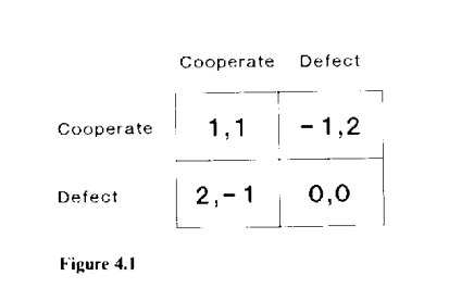
This section discusses the way in which repeated play introduces new equilibria by allowing players to condition their actions on the way their opponents played in previous periods. We begin with what is probably the best-known example of a repeated game: the celebrated “prisoner’s dilemma,” whose static version we discussed in chapter 1 . Suppose that the per-period payoffs depend only on current actions $\left(g_i\left(a^t\right)\right)$ and are as shown in figure 4.1 , and suppose that the players discount future payoffs with a common discount factor $\delta$. We will wish to consider how the equilibrium payoffs vary with the horizon $T$. To make the payoffs for different horizons comparable, we normalize to express them all in the units used for the per-period payoffs, so that the utility of a sequence $\left{a^0, \ldots, a^T\right}$ is
$$
\begin{gathered}
1-\delta \
1 \
\delta^{T+1}
\end{gathered} \sum_{i=0}^T \delta^t y_i\left(a^t\right) .
$$
This is called the “average discounted payoff.” Since the normalization is simply a rescaling, the normalized and present-value formulations represent the same preferences. The normalized versions makc it easier to see what happens as the discount factor and the time horizon vary, by measuring all payoffs in terms of per-period averages. For example, the present value of a flow of 1 per period from date 0 to date $T$ is $\left(1-\delta^{T+1}\right) /(1-\delta)$; the average discounted value of this flow is simply 1 .

We begin with the case in which the game is played only once. Then cooperating is strongly dominated, and the unique equilibrium is for both players to defect. If the game is repeated a finite number of times, subgame perfection requires both players to defect in the last period, and backward induction implies that the unique subgame-perfect equilibrium is for both players to defect in every period. $^2$

博弈论代考

经济代写|博弈论代写Game Theory代考|Backward Induction and Subgame Perfection

为了验证带有观察到的行动的多阶段游戏的策略配置文件是子游戏完美的，它足以检查是否存在任何历史$h^t$，其中一些玩家$i$可以通过在$h^t$偏离$s_i$规定的行动并遵循$s_i$而获得收益。由于这种“一阶段偏差原则”本质上是基于逆向归纳法的动态规划的最优性原则，因此它有助于说明子博弈完美性如何扩展逆向归纳法的思想。我们将观察结果分成两部分，分别对应于有限视界和无限视界游戏;有些读者可能更喜欢读第一个证明，而相信第二个证明，尽管这两个证明都很简单。为了简化符号，我们陈述了纯策略的原则;混合策略的对应物很简单。

定理4.1(有限视界博弈的一阶段偏差原理)在一个有限的多阶段博弈中，当且仅当策略剖面$s$满足一阶段偏差条件，即任何参与者$i$都不能在某一阶段偏离$s$而随后服从$s$而获得收益。更准确地说，配置文件$s$是子博弈完美的，当且仅当没有玩家$i$，也没有策略$\hat{s}i$与$s_i$一致，除了$t$和$h^t$，并且$\hat{s}_i$是$s{-i}$比$s_i$更好的响应，条件是$h^t$已经到达。 ${ }^1$

单阶段偏差条件(“只有当”)的必要性从子博弈完美性的定义出发。(请注意，一级偏差条件对于纳什均衡来说是不必要的，因为纳什均衡剖面可能会规定在历史上的次优响应，而这些响应在剖面播放时不会发生。)为了证明一级偏差条件是充分的，假设曲线相反 $s$ 满足条件，但不是完美的子博弈。然后是一个舞台 $t$ 还有一段历史 $h^t$ 这样一些玩家 $i$ 有策略 $\hat{s}i$ 这是一个更好的回应 $s{-i}$ 比 $s_i$ 是在子游戏开始的时候 $h^t$． 让 $t$ 做最大的 $t^{\prime}$ 这样，对一些人来说 $h^{\prime}, \hat{s}_i\left(h^{\prime}\right) \neq s_i\left(h^{\prime}\right)$． 一级偏差条件表示 $\hat{t}>t$，由于这个博弈是有限的， $\hat{t}$ 也是有限的。现在考虑另一种策略 $\tilde{s}_i$ 这与 $\hat{s}_i$ 一点也不 $t<\hat{t}$ 然后是 $s_i$ 舞台上 $\hat{t}$ 继续。自从 $\hat{s}_i$ 同意 $s_i$ 从 $\hat{t}+1$ On，一级偏差条件意味着 $\hat{s}_i$ 是一个好的回应吗 $\hat{s}_i$ 在每一个子游戏中 $\hat{t}$所以 $\tilde{s}_i$ 是一个好的回应吗 $\hat{S}_i$ 在子游戏开始于 $t$ 有历史 $h^t$． 如果 $\hat{t}=t+1$那么， $\tilde{s}_i=s_i$，这与假设相矛盾 $\hat{s}_i$ 改进于 $s_i$． 如果 $\hat{t}>t+1$，我们就会制定一个与之一致的策略 $\hat{s}_i$ 直到 $\hat{t}-2$． 并认为这是一个很好的回应 $\hat{s}_i$等等:所谓的改进偏差序列从它的端点开始解开。

经济代写|博弈论代写Game Theory代考|The Repeated Prisoner’s Dilemma

这一部分讨论了重复游戏如何通过允许玩家根据对手在前一阶段的行为来调整自己的行为，从而引入新的平衡。我们从重复博弈中最著名的例子开始:著名的“囚徒困境”，我们在第一章中讨论过它的静态版本。假设每个时期的收益只取决于当前的行为$\left(g_i\left(a^t\right)\right)$，如图4.1所示，并假设参与者用一个共同的贴现因子$\delta$来贴现未来的收益。我们希望考虑均衡收益如何随视界变化$T$。为了使不同层次的收益具有可比性，我们将它们归一化，用每个周期收益的单位来表示它们，因此序列$\left{a^0, \ldots, a^T\right}$的效用是
$$
\begin{gathered}
1-\delta \
1 \
\delta^{T+1}
\end{gathered} \sum_{i=0}^T \delta^t y_i\left(a^t\right) .
$$
这被称为“平均贴现收益”。由于归一化只是简单的重新缩放，因此归一化和现值公式表示相同的偏好。标准化的版本可以更容易地看到贴现因子和时间范围的变化，通过衡量每个时期的平均值的所有收益。例如，从日期0到日期$T$的每个期间1的流量的现值为$\left(1-\delta^{T+1}\right) /(1-\delta)$;这个流的平均折现值是1。

统计代写请认准statistics-lab™. statistics-lab™为您的留学生涯保驾护航。

金融工程代写

金融工程是使用数学技术来解决金融问题。金融工程使用计算机科学、统计学、经济学和应用数学领域的工具和知识来解决当前的金融问题，以及设计新的和创新的金融产品。

非参数统计代写

非参数统计指的是一种统计方法，其中不假设数据来自于由少数参数决定的规定模型；这种模型的例子包括正态分布模型和线性回归模型。

广义线性模型代考

广义线性模型（GLM）归属统计学领域，是一种应用灵活的线性回归模型。该模型允许因变量的偏差分布有除了正态分布之外的其它分布。

术语 广义线性模型（GLM）通常是指给定连续和/或分类预测因素的连续响应变量的常规线性回归模型。它包括多元线性回归，以及方差分析和方差分析（仅含固定效应）。

有限元方法代写

有限元方法（FEM）是一种流行的方法，用于数值解决工程和数学建模中出现的微分方程。典型的问题领域包括结构分析、传热、流体流动、质量运输和电磁势等传统领域。

有限元是一种通用的数值方法，用于解决两个或三个空间变量的偏微分方程（即一些边界值问题）。为了解决一个问题，有限元将一个大系统细分为更小、更简单的部分，称为有限元。这是通过在空间维度上的特定空间离散化来实现的，它是通过构建对象的网格来实现的：用于求解的数值域，它有有限数量的点。边界值问题的有限元方法表述最终导致一个代数方程组。该方法在域上对未知函数进行逼近。[1] 然后将模拟这些有限元的简单方程组合成一个更大的方程系统，以模拟整个问题。然后，有限元通过变化微积分使相关的误差函数最小化来逼近一个解决方案。

tatistics-lab作为专业的留学生服务机构，多年来已为美国、英国、加拿大、澳洲等留学热门地的学生提供专业的学术服务，包括但不限于Essay代写，Assignment代写，Dissertation代写，Report代写，小组作业代写，Proposal代写，Paper代写，Presentation代写，计算机作业代写，论文修改和润色，网课代做，exam代考等等。写作范围涵盖高中，本科，研究生等海外留学全阶段，辐射金融，经济学，会计学，审计学，管理学等全球99%专业科目。写作团队既有专业英语母语作者，也有海外名校硕博留学生，每位写作老师都拥有过硬的语言能力，专业的学科背景和学术写作经验。我们承诺100%原创，100%专业，100%准时，100%满意。

随机分析代写

随机微积分是数学的一个分支，对随机过程进行操作。它允许为随机过程的积分定义一个关于随机过程的一致的积分理论。这个领域是由日本数学家伊藤清在第二次世界大战期间创建并开始的。

时间序列分析代写

随机过程，是依赖于参数的一组随机变量的全体，参数通常是时间。 随机变量是随机现象的数量表现，其时间序列是一组按照时间发生先后顺序进行排列的数据点序列。通常一组时间序列的时间间隔为一恒定值（如1秒，5分钟，12小时，7天，1年），因此时间序列可以作为离散时间数据进行分析处理。研究时间序列数据的意义在于现实中，往往需要研究某个事物其随时间发展变化的规律。这就需要通过研究该事物过去发展的历史记录，以得到其自身发展的规律。

回归分析代写

多元回归分析渐进（Multiple Regression Analysis Asymptotics）属于计量经济学领域，主要是一种数学上的统计分析方法，可以分析复杂情况下各影响因素的数学关系，在自然科学、社会和经济学等多个领域内应用广泛。

MATLAB代写

MATLAB 是一种用于技术计算的高性能语言。它将计算、可视化和编程集成在一个易于使用的环境中，其中问题和解决方案以熟悉的数学符号表示。典型用途包括：数学和计算算法开发建模、仿真和原型制作数据分析、探索和可视化科学和工程图形应用程序开发，包括图形用户界面构建MATLAB 是一个交互式系统，其基本数据元素是一个不需要维度的数组。这使您可以解决许多技术计算问题，尤其是那些具有矩阵和向量公式的问题，而只需用 C 或 Fortran 等标量非交互式语言编写程序所需的时间的一小部分。MATLAB 名称代表矩阵实验室。MATLAB 最初的编写目的是提供对由 LINPACK 和 EISPACK 项目开发的矩阵软件的轻松访问，这两个项目共同代表了矩阵计算软件的最新技术。MATLAB 经过多年的发展，得到了许多用户的投入。在大学环境中，它是数学、工程和科学入门和高级课程的标准教学工具。在工业领域，MATLAB 是高效研究、开发和分析的首选工具。MATLAB 具有一系列称为工具箱的特定于应用程序的解决方案。对于大多数 MATLAB 用户来说非常重要，工具箱允许您学习和应用专业技术。工具箱是 MATLAB 函数（M 文件）的综合集合，可扩展 MATLAB 环境以解决特定类别的问题。可用工具箱的领域包括信号处理、控制系统、神经网络、模糊逻辑、小波、仿真等。

R语言代写	问卷设计与分析代写
PYTHON代写	回归分析与线性模型代写
MATLAB代写	方差分析与试验设计代写
STATA代写	机器学习/统计学习代写
SPSS代写	计量经济学代写
EVIEWS代写	时间序列分析代写
EXCEL代写	深度学习代写
SQL代写	各种数据建模与可视化代写

如果你也在 怎样代写博弈论Game theory 这个学科遇到相关的难题，请随时右上角联系我们的24/7代写客服。博弈论Game theory在20世纪50年代被许多学者广泛地发展。它在20世纪70年代被明确地应用于进化论，尽管类似的发展至少可以追溯到20世纪30年代。博弈论已被广泛认为是许多领域的重要工具。截至2020年，随着诺贝尔经济学纪念奖被授予博弈理论家保罗-米尔格伦和罗伯特-B-威尔逊，已有15位博弈理论家获得了诺贝尔经济学奖。约翰-梅纳德-史密斯因其对进化博弈论的应用而被授予克拉福德奖。

博弈论Game theory是对理性主体之间战略互动的数学模型的研究。它在社会科学的所有领域，以及逻辑学、系统科学和计算机科学中都有应用。最初，它针对的是两人的零和博弈，其中每个参与者的收益或损失都与其他参与者的收益或损失完全平衡。在21世纪，博弈论适用于广泛的行为关系；它现在是人类、动物以及计算机的逻辑决策科学的一个总称。

statistics-lab™ 为您的留学生涯保驾护航 在代写博弈论Game Theory方面已经树立了自己的口碑, 保证靠谱, 高质且原创的统计Statistics代写服务。我们的专家在代写博弈论Game Theory代写方面经验极为丰富，各种代写博弈论Game Theory相关的作业也就用不着说。

经济代写|博弈论代写Game Theory代考|Backward Induction and Subgame Perfection

As we have seen, the strategic form can be used to represent arbitrarily complex extensive-form games, with the strategies of the strategic form being complete contingent plans of action in the extensive form. Thus, the concept of $\mathrm{Nash}$ equilibrium can be applied to all games, not only to games where players choose their actions simultancously. However, many game theorists doubt that Nash equilibrium is the right solution concept for
8 . The existence of an optimal choice from a compact set of actions requires that payoffs be upper semi-continuous in the choice made. (A real-valued function $f(x)$ is upper semicontinuous if $x^n \rightarrow x$ implies $\lim _{n \rightarrow x} f\left(x^n\right) \leq f(x)$.) general games. In this section we will present a first look at “equilibrium refinements,” which are designed to separate the “reasonable” Nash equilibria from the “unreasonable” ones. In particular, we will discuss the ideas of backward induction and “subgame perfection.” Chapters 4, 5 and 13 apply these ideas to some classes of games of interest to economists.

Selten (1965) was the first to argue that in general extensive games some of the Nash equilibria are “more reasonable” than others. He began with the example illustrated here in figure 3.14. This is a finite game of perfect information, and the backward-induction solution (that is, the one obtained using Kuhn’s algorithm) is that player 2 should play L if his information set is reached, and so player 1 should play D. Inspection of the strategic form corresponding to this game shows that there is another Nash equilibrium, where player 1 plays $\mathrm{U}$ and player 2 plays $\mathrm{R}$. The profile $(\mathrm{U}, \mathrm{R})$ is a Nash equilibrium because, given that player 1 plays U, player 2’s information set is not reached, and player 2 loses nothing by playing $R$. But Selten argued, and we agree, that this equilibrium is suspect. After all, if player 2’s information set is reached, then, as long as player 2 is convinced that his payoffs are as specified in the figure, player 2 should play L. And if we were player 2, this is how we would play. Moreover, if we were player 1, we would expect player 2 to play $\mathrm{L}$, and so we would play $\mathrm{D}$.

In the now-familiar language, the equilibrium $(\mathbf{U}, \mathbf{R})$ is not “credible,” because it relies on an “empty threat” by player 2 to play R. The threat is “empty” because player 2 would never wish to carry it out.

经济代写|博弈论代写Game Theory代考|C’ritiques of Backward Induction

Consider the 1 -player game illustrated in figure 3.18, where each player $i<I$ can either end the game by playing ” $D$ ” or play ” $A$ ” and give the move to player $i+1$. (To readers who skipped sections 3.3-3.5: Figure 3.18 depicts a “game tree.” Though you have not seen a formal definition of such trees, we trust that the particular trees we use in this subsection will be clear.) If player $i$ plays D, each player gets $1 / i$; if all players play A, cach gets 2 .

Since only onc player moves at a time, this is a game of perfect information, and we can apply the backward-induction algorithm, which predicts that all players should play $A$. If $I$ is small, this seems like a reasonable prediction. If $I$ is very large, then, as player 1 , we ourselves would play D and not A on the basis of a “robustness” argument similar to the one that suggested the inefficient equilibrium in the stag-hunt game of subsection 1.2 .4 .

First, the payoff 2 requires that all $I-1$ other players play $A$. If the probability that a given player plays $A$ is $p<1$, independent of the others. the probability that all $I-1$ other players play $\mathrm{A}$ is $p^I{ }^1$, which can be quite small even if $p$ is very large. Second, we would worry that player 2 might have these same concerns; that is, player 2 might play D to safeguard against either “mistakes” by future players or the possibility that player 3 might intentionally play $\mathrm{D}$.

A related observation is that longer chains of backward induction presume longer chains of the hypothesis that “player 1 knows that player 2 knows that player 3 knows… the payoffs.” If $I=2$ in figure 3.18 , backward induction supposes that player 1 knows player 2 ‘s payoff, or at least that player 1 is fairly sure that player 2 ‘s optimal choice is A. If $I=3$, not only must players 1 and 2 know player 3 ‘s payoff, in addition, player 1 must know that player 2 knows player 3’s payoff, so that player 1 can forecast player 2’s forecast of player 3’s play. If player 1 thinks that player 2 will forecast player 3 ‘s play incorrectly, then player 1 may choose to play D.

博弈论代考

经济代写|博弈论代写Game Theory代考|Backward Induction and Subgame Perfection

正如我们所看到的，战略形式可以用来表示任意复杂的广泛形式博弈，战略形式的策略是广泛形式中完整的偶然行动计划。因此，$\mathrm{Nash}$均衡概念可以应用于所有游戏，而不仅仅是玩家同时选择行动的游戏。然而，许多博弈论家怀疑纳什均衡是否是解决问题的正确概念
8。从一组紧致的行动中存在最优选择，要求所作选择的收益是上半连续的。(如果$x^n \rightarrow x$暗示$\lim _{n \rightarrow x} f\left(x^n\right) \leq f(x)$，则实值函数$f(x)$是上半连续的。)在本节中，我们将首先介绍“均衡优化”，它旨在将“合理的”纳什均衡与“不合理的”纳什均衡区分开来。特别地，我们将讨论逆向归纳法和“子博弈完善”的思想。第4章、第5章和第13章将这些思想应用于经济学家感兴趣的一些游戏类。

Selten(1965)是第一个提出在一般广泛博弈中，某些纳什均衡比其他均衡“更合理”的人。他从图3.14所示的例子开始。这是一个完全信息的有限博弈，逆向归纳解(即使用库恩算法获得的解)是，如果达到参与人2的信息集，参与人2应该选择L，因此参与人1应该选择d。检查该博弈对应的策略形式表明，存在另一个纳什均衡，其中参与人1选择$\mathrm{U}$，参与人2选择$\mathrm{R}$。配置文件$(\mathrm{U}, \mathrm{R})$是纳什均衡，因为假设参与人1选择U，参与人2的信息集不会达到，参与人2选择$R$不会损失任何东西。但塞尔滕认为，这种均衡是可疑的，我们也同意这一点。毕竟，如果达到了参与人2的信息集，那么，只要参与人2确信他的收益如图中所示，参与人2就应该选择l，如果我们是参与人2，我们就会这么玩。此外，如果我们是参与人1，我们会期望参与人2玩$\mathrm{L}$，所以我们会玩$\mathrm{D}$。

用现在熟悉的语言来说，均衡$(\mathbf{U}, \mathbf{R})$是不“可信的”，因为它依赖于玩家2对r的“空威胁”。威胁是“空的”，因为玩家2永远不会想要执行它。

经济代写|博弈论代写Game Theory代考|C’ritiques of Backward Induction

考虑图3.18所示的1人博弈，其中每个玩家$i<I$可以通过“$D$”结束游戏，也可以通过“$A$”结束游戏，并将移动权交给玩家$i+1$。(对于跳过3.3-3.5节的读者:图3.18描绘了一个“游戏树”。虽然您还没有看到这种树的正式定义，但我们相信在本小节中使用的特定树将是清楚的。)如果玩家$i$选择D，每个玩家都得到$1 / i$;如果所有人都选A，每人得2分。

由于一次只有一个玩家移动，这是一个完全信息的博弈，我们可以应用反向归纳算法，该算法预测所有玩家都应该玩$A$。如果$I$很小，这似乎是一个合理的预测。如果$I$非常大，那么作为参与人1，我们自己就会选择D而不是A，这是基于“稳健性”论证，类似于第1.2 .4小节中提出的猎鹿博弈中的低效均衡。

首先，收益2要求所有$I-1$其他玩家都玩$A$。如果给定玩家选择$A$的概率是$p<1$，与其他玩家无关。所有$I-1$其他玩家都玩$\mathrm{A}$的概率是$p^I{ }^1$，即使$p$很大，这个概率也很小。其次，我们会担心玩家2也会有同样的担忧;也就是说，玩家2可能会选择D，以防止未来玩家的“错误”，或者玩家3可能会故意选择$\mathrm{D}$。

一个相关的观察是，更长的逆向归纳链假设了更长的假设链，即“参与人1知道参与人2知道参与人3知道……收益”。如果在图3.18中$I=2$，逆向归纳假设参与人1知道参与人2的收益，或者至少参与人1相当确定参与人2的最优选择是a。如果$I=3$，不仅参与人1和参与人2必须知道参与人3的收益，另外，参与人1必须知道参与人2知道参与人3的收益，这样参与人1就可以预测参与人2对参与人3的收益的预测。如果参与人1认为参与人2会错误地预测参与人3的策略，那么参与人1可能会选择D。

统计代写请认准statistics-lab™. statistics-lab™为您的留学生涯保驾护航。

金融工程代写

金融工程是使用数学技术来解决金融问题。金融工程使用计算机科学、统计学、经济学和应用数学领域的工具和知识来解决当前的金融问题，以及设计新的和创新的金融产品。

非参数统计代写

非参数统计指的是一种统计方法，其中不假设数据来自于由少数参数决定的规定模型；这种模型的例子包括正态分布模型和线性回归模型。

广义线性模型代考

广义线性模型（GLM）归属统计学领域，是一种应用灵活的线性回归模型。该模型允许因变量的偏差分布有除了正态分布之外的其它分布。

术语 广义线性模型（GLM）通常是指给定连续和/或分类预测因素的连续响应变量的常规线性回归模型。它包括多元线性回归，以及方差分析和方差分析（仅含固定效应）。

有限元方法代写

有限元方法（FEM）是一种流行的方法，用于数值解决工程和数学建模中出现的微分方程。典型的问题领域包括结构分析、传热、流体流动、质量运输和电磁势等传统领域。

有限元是一种通用的数值方法，用于解决两个或三个空间变量的偏微分方程（即一些边界值问题）。为了解决一个问题，有限元将一个大系统细分为更小、更简单的部分，称为有限元。这是通过在空间维度上的特定空间离散化来实现的，它是通过构建对象的网格来实现的：用于求解的数值域，它有有限数量的点。边界值问题的有限元方法表述最终导致一个代数方程组。该方法在域上对未知函数进行逼近。[1] 然后将模拟这些有限元的简单方程组合成一个更大的方程系统，以模拟整个问题。然后，有限元通过变化微积分使相关的误差函数最小化来逼近一个解决方案。

tatistics-lab作为专业的留学生服务机构，多年来已为美国、英国、加拿大、澳洲等留学热门地的学生提供专业的学术服务，包括但不限于Essay代写，Assignment代写，Dissertation代写，Report代写，小组作业代写，Proposal代写，Paper代写，Presentation代写，计算机作业代写，论文修改和润色，网课代做，exam代考等等。写作范围涵盖高中，本科，研究生等海外留学全阶段，辐射金融，经济学，会计学，审计学，管理学等全球99%专业科目。写作团队既有专业英语母语作者，也有海外名校硕博留学生，每位写作老师都拥有过硬的语言能力，专业的学科背景和学术写作经验。我们承诺100%原创，100%专业，100%准时，100%满意。

随机分析代写

随机微积分是数学的一个分支，对随机过程进行操作。它允许为随机过程的积分定义一个关于随机过程的一致的积分理论。这个领域是由日本数学家伊藤清在第二次世界大战期间创建并开始的。

时间序列分析代写

随机过程，是依赖于参数的一组随机变量的全体，参数通常是时间。 随机变量是随机现象的数量表现，其时间序列是一组按照时间发生先后顺序进行排列的数据点序列。通常一组时间序列的时间间隔为一恒定值（如1秒，5分钟，12小时，7天，1年），因此时间序列可以作为离散时间数据进行分析处理。研究时间序列数据的意义在于现实中，往往需要研究某个事物其随时间发展变化的规律。这就需要通过研究该事物过去发展的历史记录，以得到其自身发展的规律。

回归分析代写

多元回归分析渐进（Multiple Regression Analysis Asymptotics）属于计量经济学领域，主要是一种数学上的统计分析方法，可以分析复杂情况下各影响因素的数学关系，在自然科学、社会和经济学等多个领域内应用广泛。

MATLAB代写

MATLAB 是一种用于技术计算的高性能语言。它将计算、可视化和编程集成在一个易于使用的环境中，其中问题和解决方案以熟悉的数学符号表示。典型用途包括：数学和计算算法开发建模、仿真和原型制作数据分析、探索和可视化科学和工程图形应用程序开发，包括图形用户界面构建MATLAB 是一个交互式系统，其基本数据元素是一个不需要维度的数组。这使您可以解决许多技术计算问题，尤其是那些具有矩阵和向量公式的问题，而只需用 C 或 Fortran 等标量非交互式语言编写程序所需的时间的一小部分。MATLAB 名称代表矩阵实验室。MATLAB 最初的编写目的是提供对由 LINPACK 和 EISPACK 项目开发的矩阵软件的轻松访问，这两个项目共同代表了矩阵计算软件的最新技术。MATLAB 经过多年的发展，得到了许多用户的投入。在大学环境中，它是数学、工程和科学入门和高级课程的标准教学工具。在工业领域，MATLAB 是高效研究、开发和分析的首选工具。MATLAB 具有一系列称为工具箱的特定于应用程序的解决方案。对于大多数 MATLAB 用户来说非常重要，工具箱允许您学习和应用专业技术。工具箱是 MATLAB 函数（M 文件）的综合集合，可扩展 MATLAB 环境以解决特定类别的问题。可用工具箱的领域包括信号处理、控制系统、神经网络、模糊逻辑、小波、仿真等。

R语言代写	问卷设计与分析代写
PYTHON代写	回归分析与线性模型代写
MATLAB代写	方差分析与试验设计代写
STATA代写	机器学习/统计学习代写
SPSS代写	计量经济学代写
EVIEWS代写	时间序列分析代写
EXCEL代写	深度学习代写
SQL代写	各种数据建模与可视化代写

如果你也在 怎样代写博弈论Game theory 这个学科遇到相关的难题，请随时右上角联系我们的24/7代写客服。博弈论Game theory在20世纪50年代被许多学者广泛地发展。它在20世纪70年代被明确地应用于进化论，尽管类似的发展至少可以追溯到20世纪30年代。博弈论已被广泛认为是许多领域的重要工具。截至2020年，随着诺贝尔经济学纪念奖被授予博弈理论家保罗-米尔格伦和罗伯特-B-威尔逊，已有15位博弈理论家获得了诺贝尔经济学奖。约翰-梅纳德-史密斯因其对进化博弈论的应用而被授予克拉福德奖。

博弈论Game theory是对理性主体之间战略互动的数学模型的研究。它在社会科学的所有领域，以及逻辑学、系统科学和计算机科学中都有应用。最初，它针对的是两人的零和博弈，其中每个参与者的收益或损失都与其他参与者的收益或损失完全平衡。在21世纪，博弈论适用于广泛的行为关系；它现在是人类、动物以及计算机的逻辑决策科学的一个总称。

statistics-lab™ 为您的留学生涯保驾护航 在代写博弈论Game Theory方面已经树立了自己的口碑, 保证靠谱, 高质且原创的统计Statistics代写服务。我们的专家在代写博弈论Game Theory代写方面经验极为丰富，各种代写博弈论Game Theory相关的作业也就用不着说。

经济代写|博弈论代写Game Theory代考|Behavior Strategies

This section defines strategies and equilibria in extensive-form games and relates them to strategies and equilibria of the strategic-form model. Let $H_i$ be the set of player $i$ ‘s information sets, and let $A_i \equiv \bigcup_{h_i \in H_i} A\left(h_i\right)$ be the set of all actions for player $i$. A pure strategy for player $i$ is a map $s_i: H_i \rightarrow A_i$, with $s_i\left(h_i\right) \in A\left(h_i\right)$ for all $h_i \in H_i$. Player $i$ ‘s space of pure strategies, $S_i$, is simply the space of all such $s_i$. Since each pure strategy is at map from information sets to actions, we can write $S_i$ as the Cartesian product of the action spaces at each $h_i$ :
$$
S_i=\underset{h_i \in H_i}{\times} A\left(h_i\right) .
$$
In the Stackelberg example of figure 3.3, player 1 has a single information set and three actions, so that he has three pure strategies. Player 2 has three information sets, corresponding to the three possible choices of player 1 , and player 2 has three possible actions at each information set, so player 2 has 27 pure strategies in all. More generally, the number of player $i$ ‘s pure strategies, # $S_i$, equals
$$
\prod_{h_i \in H_i} #\left(A\left(h_i\right)\right) \text {. }
$$
Given a pure strategy for each player $i$ and the probability distribution over Nature’s moves, we can compute a probability distribution over outcomes and thus assign expected payoffs $u_i(s)$ to each strategy profile $s$. The information sets that are reached with positive probability under profile $s$ are called the path of $s$.

Now that we have defined the payoffs to each pure strategy, we can proceed to define a pure-strategy Nash equilibrium for an extensive-form game as a strategy profile $s^$ such that each player $i$ ‘s strategy $s_i^$ maximizes his expected payoff given the strategies $s_{-i}^*$ of his opponents. Note that since the definition of Nash equilibrium holds the strategies of player $i$ ‘s opponents fixed in testing whether player $i$ wishes to deviate, it is as if the players choose their strategies simultaneously. This does not mean that in Nash equilibrium players necessarily choose their actions simultaneously. For example, if player 2’s fixed strategy in the Stackelberg game of figure 3.3 is the Cournot reaction function $\hat{s}_2=(4,4,3)$, then when player 1 treats player 2’s strategy as fixed he does not presume that player 2’s action is unaffected by his own, but rather that player 2 will respond to player 1’s action in the way specified by $\hat{S}_2$.

经济代写|博弈论代写Game Theory代考|The Strategic-Form Representation of Extensive-Form Games

Our next step is to relate extensive-form games and equilibria to the strategic-form model. To define a strategic form from an extensive form, we simply let the pure strategies $s \in S$ and the payoffs $u_i(s)$ be exactly those we defined in the extensive form. A different way of saying this is that the same pure strategies can be interpreted as either extensive-form or strategic-form objects. With the extensive-form interpretation, player $i$ “waits” until $h_i$ is reached before deciding how to play there; with the strategic-form interpretation, he makes a complete contingent plan in advance.

Figure 3.8 illustrates this passage from the extensive form to the strategic form in a simple example. We order player 2’s information sets from left to right, so that, for example, the strategy $s_2=(\mathrm{L}, \mathrm{R})$ means that he plays $L$ after $L^{\prime}$ and $R$ after D.

As another example, consider the Stackelberg game illustrated in figure 3.3. We will again order player 2’s information sets from left to right, so that player 2 ‘s strategy $\hat{s}_2=(4,4,3)$ means that he plays 4 in response to $q_1=3$, plays 4 in response to 4 , and plays 3 in response to 6 . (This strategy happens to be player 2’s Cournot reaction function.) Since player 2 has three information sets and three possible actions at each of these sets, he has 27 pure strategies. We trust that the reader will forgive our not displaying the strategic form in a matrix diagram!

There can be several extensive forms with the same strategic form, as the example of simultaneous moves shows: Figures $3.4 \mathrm{a}$ and $3.4 \mathrm{~b}$ both correspond to the same strategic form for the Cournot game.

At this point we should note that the strategy space as we have defined it may be unnecessarily large, as it may contain pairs of strategies that are “equivalent” in the sense of having the same consequences regardless of how the opponents play.

博弈论代考

经济代写|博弈论代写Game Theory代考|Behavior Strategies

本节定义了广泛形式博弈中的策略和均衡，并将它们与策略形式模型中的策略和均衡联系起来。设$H_i$为玩家$i$的信息集合，设$A_i \equiv \bigcup_{h_i \in H_i} A\left(h_i\right)$为玩家$i$的所有动作集合。玩家$i$的纯策略是一张地图$s_i: H_i \rightarrow A_i$, $s_i\left(h_i\right) \in A\left(h_i\right)$代表所有的$h_i \in H_i$。参与人$i$的纯策略空间$S_i$，就是所有这些的空间$s_i$。由于每个纯策略都是从信息集映射到行动，我们可以将$S_i$写成每个$h_i$处的行动空间的笛卡尔积:
$$
S_i=\underset{h_i \in H_i}{\times} A\left(h_i\right) .
$$
在图3.3的Stackelberg例子中，参与人1有一个信息集和三个行动，所以他有三个纯策略。参与人2有三个信息集，对应于参与人1的三种可能选择，参与人2在每个信息集有三种可能的行动，因此参与人2总共有27种纯策略。更一般地说，玩家$i$的纯策略数量，＃ $S_i$等于
$$
\prod_{h_i \in H_i} #\left(A\left(h_i\right)\right) \text {. }
$$
给定每个玩家的纯策略$i$和自然移动的概率分布，我们可以计算结果的概率分布，从而为每个策略配置文件$s$分配预期收益$u_i(s)$。在概要文件$s$下以正概率到达的信息集称为$s$的路径。

既然我们已经定义了每种纯策略的收益，我们就可以将广义博弈的纯策略纳什均衡定义为策略概要$s^$，使得每个参与人$i$的策略$s_i^$在给定其对手的策略$s_{-i}^*$的情况下最大化其预期收益。请注意，由于纳什均衡的定义在测试参与人$i$是否希望偏离时，将参与人$i$对手的策略固定下来，这就好像参与人同时选择了他们的策略。这并不意味着在纳什均衡中，参与者必须同时选择他们的行动。例如，如果在图3.3的Stackelberg博弈中，参与人2的固定策略是古诺反应函数$\hat{s}_2=(4,4,3)$，那么当参与人1将参与人2的策略视为固定策略时，他不会假设参与人2的行动不受自己的影响，而是认为参与人2将以$\hat{S}_2$指定的方式对参与人1的行动做出反应。

经济代写|博弈论代写Game Theory代考|The Strategic-Form Representation of Extensive-Form Games

我们的下一步是将广泛形式的博弈和均衡与战略形式的模型联系起来。为了从扩展形式中定义策略形式，我们简单地让纯策略$s \in S$和收益$u_i(s)$与我们在扩展形式中定义的完全相同。换句话说，同样的纯策略既可以被解释为外延形式客体，也可以被解释为策略形式客体。根据广义解释，玩家$i$“等待”到$h_i$才决定如何在那里玩;在战略形式的解释下，他提前制定了一个完整的应急计划。

图3.8用一个简单的例子说明了从外延形式到策略形式的转变。我们将参与人2的信息集从左到右排序，因此，例如，策略$s_2=(\mathrm{L}, \mathrm{R})$意味着他在$L^{\prime}$之后选择$L$，在D之后选择$R$。

另一个例子是图3.3所示的Stackelberg游戏。我们将再次对参与人2的信息集从左到右排序，因此参与人2的策略$\hat{s}_2=(4,4,3)$意味着他对$q_1=3$的回应是4，对4的回应是4，对6的回应是3。(这个策略恰好是参与人2的古诺反应函数。)因为参与人2有三个信息集，每个信息集有三个可能的行动，所以他有27个纯策略。我们相信读者会原谅我们没有在矩阵图中展示战略形式!

可以有几种具有相同策略形式的扩展形式，如同时移动的例子所示:图$3.4 \mathrm{a}$和$3.4 \mathrm{~b}$都对应于古诺博弈的相同策略形式。

在这一点上，我们应该注意到我们所定义的策略空间可能是不必要的大，因为它可能包含“等效”的策略对，即无论对手如何操作都具有相同的结果。

统计代写请认准statistics-lab™. statistics-lab™为您的留学生涯保驾护航。

金融工程代写

金融工程是使用数学技术来解决金融问题。金融工程使用计算机科学、统计学、经济学和应用数学领域的工具和知识来解决当前的金融问题，以及设计新的和创新的金融产品。

非参数统计代写

非参数统计指的是一种统计方法，其中不假设数据来自于由少数参数决定的规定模型；这种模型的例子包括正态分布模型和线性回归模型。

广义线性模型代考

广义线性模型（GLM）归属统计学领域，是一种应用灵活的线性回归模型。该模型允许因变量的偏差分布有除了正态分布之外的其它分布。

术语 广义线性模型（GLM）通常是指给定连续和/或分类预测因素的连续响应变量的常规线性回归模型。它包括多元线性回归，以及方差分析和方差分析（仅含固定效应）。

有限元方法代写

有限元方法（FEM）是一种流行的方法，用于数值解决工程和数学建模中出现的微分方程。典型的问题领域包括结构分析、传热、流体流动、质量运输和电磁势等传统领域。

有限元是一种通用的数值方法，用于解决两个或三个空间变量的偏微分方程（即一些边界值问题）。为了解决一个问题，有限元将一个大系统细分为更小、更简单的部分，称为有限元。这是通过在空间维度上的特定空间离散化来实现的，它是通过构建对象的网格来实现的：用于求解的数值域，它有有限数量的点。边界值问题的有限元方法表述最终导致一个代数方程组。该方法在域上对未知函数进行逼近。[1] 然后将模拟这些有限元的简单方程组合成一个更大的方程系统，以模拟整个问题。然后，有限元通过变化微积分使相关的误差函数最小化来逼近一个解决方案。

tatistics-lab作为专业的留学生服务机构，多年来已为美国、英国、加拿大、澳洲等留学热门地的学生提供专业的学术服务，包括但不限于Essay代写，Assignment代写，Dissertation代写，Report代写，小组作业代写，Proposal代写，Paper代写，Presentation代写，计算机作业代写，论文修改和润色，网课代做，exam代考等等。写作范围涵盖高中，本科，研究生等海外留学全阶段，辐射金融，经济学，会计学，审计学，管理学等全球99%专业科目。写作团队既有专业英语母语作者，也有海外名校硕博留学生，每位写作老师都拥有过硬的语言能力，专业的学科背景和学术写作经验。我们承诺100%原创，100%专业，100%准时，100%满意。

随机分析代写

随机微积分是数学的一个分支，对随机过程进行操作。它允许为随机过程的积分定义一个关于随机过程的一致的积分理论。这个领域是由日本数学家伊藤清在第二次世界大战期间创建并开始的。

时间序列分析代写

随机过程，是依赖于参数的一组随机变量的全体，参数通常是时间。 随机变量是随机现象的数量表现，其时间序列是一组按照时间发生先后顺序进行排列的数据点序列。通常一组时间序列的时间间隔为一恒定值（如1秒，5分钟，12小时，7天，1年），因此时间序列可以作为离散时间数据进行分析处理。研究时间序列数据的意义在于现实中，往往需要研究某个事物其随时间发展变化的规律。这就需要通过研究该事物过去发展的历史记录，以得到其自身发展的规律。

回归分析代写

多元回归分析渐进（Multiple Regression Analysis Asymptotics）属于计量经济学领域，主要是一种数学上的统计分析方法，可以分析复杂情况下各影响因素的数学关系，在自然科学、社会和经济学等多个领域内应用广泛。

MATLAB代写

MATLAB 是一种用于技术计算的高性能语言。它将计算、可视化和编程集成在一个易于使用的环境中，其中问题和解决方案以熟悉的数学符号表示。典型用途包括：数学和计算算法开发建模、仿真和原型制作数据分析、探索和可视化科学和工程图形应用程序开发，包括图形用户界面构建MATLAB 是一个交互式系统，其基本数据元素是一个不需要维度的数组。这使您可以解决许多技术计算问题，尤其是那些具有矩阵和向量公式的问题，而只需用 C 或 Fortran 等标量非交互式语言编写程序所需的时间的一小部分。MATLAB 名称代表矩阵实验室。MATLAB 最初的编写目的是提供对由 LINPACK 和 EISPACK 项目开发的矩阵软件的轻松访问，这两个项目共同代表了矩阵计算软件的最新技术。MATLAB 经过多年的发展，得到了许多用户的投入。在大学环境中，它是数学、工程和科学入门和高级课程的标准教学工具。在工业领域，MATLAB 是高效研究、开发和分析的首选工具。MATLAB 具有一系列称为工具箱的特定于应用程序的解决方案。对于大多数 MATLAB 用户来说非常重要，工具箱允许您学习和应用专业技术。工具箱是 MATLAB 函数（M 文件）的综合集合，可扩展 MATLAB 环境以解决特定类别的问题。可用工具箱的领域包括信号处理、控制系统、神经网络、模糊逻辑、小波、仿真等。

R语言代写	问卷设计与分析代写
PYTHON代写	回归分析与线性模型代写
MATLAB代写	方差分析与试验设计代写
STATA代写	机器学习/统计学习代写
SPSS代写	计量经济学代写
EVIEWS代写	时间序列分析代写
EXCEL代写	深度学习代写
SQL代写	各种数据建模与可视化代写