标签: ES4C5

物理代写|光学工程代写Optical Engineering代考|EGEE480

如果你也在 怎样代写光学工程Optical Engineering这个学科遇到相关的难题,请随时右上角联系我们的24/7代写客服。

光学工程是科学和工程领域,包括与光的产生、传输、操纵、检测和利用有关的物理现象和技术。

statistics-lab™ 为您的留学生涯保驾护航 在代写光学工程Optical Engineering方面已经树立了自己的口碑, 保证靠谱, 高质且原创的统计Statistics代写服务。我们的专家在代写光学工程Optical Engineering代写方面经验极为丰富,各种代写光学工程Optical Engineering相关的作业也就用不着说。

我们提供的光学工程Optical Engineering及其相关学科的代写,服务范围广, 其中包括但不限于:

  • Statistical Inference 统计推断
  • Statistical Computing 统计计算
  • Advanced Probability Theory 高等概率论
  • Advanced Mathematical Statistics 高等数理统计学
  • (Generalized) Linear Models 广义线性模型
  • Statistical Machine Learning 统计机器学习
  • Longitudinal Data Analysis 纵向数据分析
  • Foundations of Data Science 数据科学基础
物理代写|光学工程代写Optical Engineering代考|EGEE480

物理代写|光学工程代写Optical Engineering代考|Interference and Diffraction

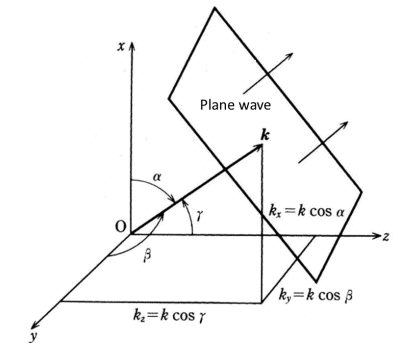
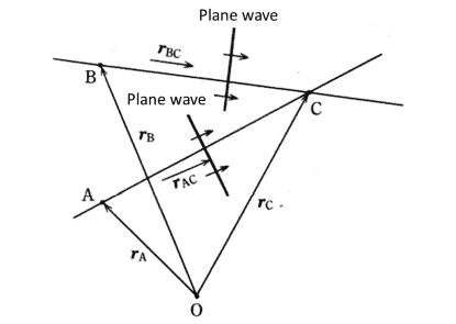
Consider two sinusoidal waves passing from point $\mathrm{A}$ to point $\mathrm{C}$ and from point $\mathrm{B}$ to point C. For simplicity, the frequencies of the two waves are the same. Vectors of AC and $\mathrm{BC}$ are denoted by $\boldsymbol{r}{A C}$ and $\boldsymbol{r}{B C}$, respectively, and their wave number vectors by $\boldsymbol{k}A$ and $\boldsymbol{k}_B$, respectively (see Fig. 2.1). The plane wave arriving at point $\mathrm{C}$ from point $A$ is given by $$ u_A=A_A \exp \left[\mathbf{i}\left(\boldsymbol{k}_A \cdot \boldsymbol{r}{A C}+\phi_A-\omega t\right)\right],
$$
and the plane wave arriving at point $\mathrm{C}$ from point $\mathrm{B}$ is
$$
u_B=A_B \exp \left[\mathrm{i}\left(\boldsymbol{k}B \cdot \boldsymbol{r}{B C}+\phi_B-\omega t\right)\right] .
$$
Suppose the position vectors of points A and C are $\boldsymbol{r}A\left(x_A, y_A, z_A\right)$ and $\boldsymbol{r}_C\left(x_C, y_C, z_C\right)$, we have $$ r{A C}=r_C-r_A .
$$
By using Eq. (1.30), we have
$$
\begin{aligned}
\boldsymbol{k}A \cdot \boldsymbol{r}{A C} & =\boldsymbol{k} \cdot\left(\boldsymbol{r}C-\boldsymbol{r}_A\right) \ & =\frac{2 \pi}{\lambda_0} n\left[\left(x_C-x_A\right) \cos \alpha_A+\left(y_C-y_A\right) \cos \beta_A+\left(z_C-z_A\right) \cos \gamma_A\right], \end{aligned} $$ where the directional cosines of the vector $\boldsymbol{k}_A$ are $\left(\cos \alpha_A, \cos \beta_A, \cos \gamma_A\right)$. If $$ \left(x_C-x_A\right) \cos \alpha_A+\left(y_C-y_A\right) \cos \beta_A+\left(z_C-z_A\right) \cos \gamma_A=l{A C},
$$
then $l_{A C}$ gives the distance between points A and $\mathrm{C}$, and $n l_{A C}$ is called the optical distance, where $n$ is the refractive index of the medium. Equations (2.1) and (2.2) are rewritten as
$$
u_A=A_A \exp \left[\mathrm{i}\left(\frac{2 \pi}{\lambda_0} n l_{A C}+\phi_A-\omega t\right)\right]
$$ and
$$
u_B=A_B \exp \left[\mathrm{i}\left(\frac{2 \pi}{\lambda_0} n l_{B C}+\phi_B-\omega t\right)\right],
$$
respectively. Since the amplitude $u_C$ at point $\mathrm{C}$ is given by the superposition of two waves $u_A$ and $u_B$, we have
$$
\begin{aligned}
u_C & =A_A \exp \left[\mathrm{i}\left(\frac{2 \pi}{\lambda_0} n l_{A C}+\phi_A-\omega t\right)\right]+A_B \exp \left[\mathrm{i}\left(\frac{2 \pi}{\lambda_0} n l_{B C}+\phi_B-\omega t\right)\right] \
& =\left{A_A \exp \left[\mathrm{i}\left(\frac{2 \pi}{\lambda_0} n l_{A C}+\phi_A\right)\right]+A_B \exp \left[\mathrm{i}\left(\frac{2 \pi}{\lambda_0} n l_{B C}+\phi_B\right)\right]\right} \exp (-\mathrm{i} \omega t)
\end{aligned}
$$

物理代写|光学工程代写Optical Engineering代考|FRINGE VISIBILITY

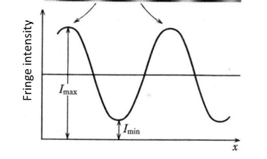
As the measure of interference fringe clarity, the contrast or the visibility is defined by
$$
V=\frac{I_{\max }-I_{\min }}{I_{\max }+I_{\min }},
$$
where $I_{\max }$ and $I_{\min }$ are the maximum and the minimum of the fringe intensity, respectively. We have
$$
V=\frac{2 \sqrt{I_A I_B}}{I_A+I_B}
$$ by using Eq. (2.9). The maximum contrast of $V=1$ is obtained when $I_A=I_B$. When either $I_A$ or $I_B$ is 0 , the minimum $V=0$ so that the fringe is invisible.

Whenever $A_A=A_B$, is the contrast always $V=1$ ? In reality, a special condition is necessary for $V=1$. The interference fringe exists stably in time, only when the difference $\phi_B-\phi_A$ of the initial phase of $\phi_A$ and $\phi_B$ at the point A and B is stable in time. The difference $\phi_B-\phi_A$ depends on the properties of the light sources, the distances from the light source to the point A and B, and so on. This means the contrast of the interference fringe depends not only on the path difference of $l_{B C}-l_{A C}$ but also the light source properties and the layout of the optical system.

The phase of wave from the light source in many cases is stable in less than $10^{-8}$ seconds. We can see the wave shape is sinusoidal only within this short time, where the amplitude and the phase are fixed within an appropriate time. Many wavelets with fixed duration generated from the light source form practical waves. From this concept, to generate a stable interference fringe at point $\mathrm{C}$, the waves A and B departing from the same source and at the same time should superimpose at point $\mathrm{C}$. The device used to perform such a superposition is called as an interferometer.
As described in Section 10.1, the stability of the phase difference $\phi_B-\phi_A$ depends on the properties of the light source. The measure is called the degree of coherence, $\gamma_{A B}$. We have $0 \leq \gamma_{A B} \leq 1$. In the case of $\gamma_{A B}=1$, two waves from the point $A$ and B are called coherent each other, and incoherent in the case of $\gamma_{A B}=0$. When considering the coherence, the fringe contract is rewritten as
$$
V=\frac{2 \sqrt{I_A I_B}}{I_A+I_B} \gamma_{A B} .
$$

物理代写|光学工程代写Optical Engineering代考|EGEE480

光学工程代考

物理代写|光学工程代写Optical Engineering代考|Interference and Diffraction

考虑从点传递的两个正弦波 $A$ 指向 $C$ 从点B到C点。为简单起见,两个波的频率相同。AC 的向 量和 $\mathrm{BC}$ 表示为 $r A C$ 和 $r B C$ ,分别和它们的波数向量 $k A$ 和 $\boldsymbol{k}B$ ,分别 (见图 2.1)。到达点 的平面波C从点 $A$ 是 (谁) 给的 $$ u_A=A_A \exp \left[\mathbf{i}\left(\boldsymbol{k}_A \cdot \boldsymbol{r} A C+\phi_A-\omega t\right)\right], $$ 平面波到达点 $\mathrm{C}$ 从点 $\mathrm{B}$ 是 $$ u_B=A_B \exp \left[\mathrm{i}\left(\boldsymbol{k} B \cdot \boldsymbol{r} B C+\phi_B-\omega t\right)\right] . $$ 假设点 $\mathrm{A}$ 和 C 的位置向量是 $\boldsymbol{r} A\left(x_A, y_A, z_A\right)$ 和 $\boldsymbol{r}_C\left(x_C, y_C, z_C\right)$ ,我们有 $$ r A C=r_C-r_A . $$ 通过使用等式。(1.30),我们有 $$ \boldsymbol{k} A \cdot \boldsymbol{r} A C=\boldsymbol{k} \cdot\left(\boldsymbol{r} C-\boldsymbol{r}_A\right) \quad=\frac{2 \pi}{\lambda_0} n\left[\left(x_C-x_A\right) \cos \alpha_A+\left(y_C-y_A\right) \cos \beta_A+\left(z_C\right.\right. $$ 其中矢量的方向余弦 $\boldsymbol{k}_A$ 是 $\left(\cos \alpha_A, \cos \beta_A, \cos \gamma_A\right)$. 如果 $$ \left(x_C-x_A\right) \cos \alpha_A+\left(y_C-y_A\right) \cos \beta_A+\left(z_C-z_A\right) \cos \gamma_A=l A C, $$ 然后 $l{A C}$ 给出点 $\mathrm{A}$ 和 C,和 $n l_{A C}$ 称为光学距离,其中 $n$ 是介质的折射率。等式 (2.1) 和 (2.2) 改写为
$$
u_A=A_A \exp \left[\mathrm{i}\left(\frac{2 \pi}{\lambda_0} n l_{A C}+\phi_A-\omega t\right)\right]
$$

$$
u_B=A_B \exp \left[\mathrm{i}\left(\frac{2 \pi}{\lambda_0} n l_{B C}+\phi_B-\omega t\right)\right],
$$
分别。由于振幅 $u_C$ 在点C由两个波的叠加给出 $u_A$ 和 $u_B$.

物理代写|光学工程代写Optical Engineering代考|FRINGE VISIBILITY

作为干涉条纹靓晰度的衡量标准,对比度或可见度定义为
$$
V=\frac{I_{\max }-I_{\min }}{I_{\max }+I_{\min }},
$$
在哪里 $I_{\max }$ 和 $I_{\min }$ 分别是条纹强度的最大值和最小值。我们有
$$
V=\frac{2 \sqrt{I_A I_B}}{I_A+I_B}
$$
通过使用等式。(2.9)。最大对比度 $V=1$ 获得时 $I_A=I_B$. 当 $I_A$ 要么 $I_B$ 为 0 ,最小 $V=0$ 这 样边缘就看不见了。
每当 $A_A=A_B$ ,总是对比 $V=1$ ? 实际上,需要一个特殊的条件 $V=1$. 干涉条纹在时间上 稳定存在,只有当差异 $\phi_B-\phi_A$ 的初始阶段 $\phi_A$ 和 $\phi_B \mathrm{~A}$ 点和B点在时间上是稳定的。区别 $\phi_B-\phi_A$ 取决于光源的属性、光源到点 $\mathrm{A}$ 和 $\mathrm{B}$ 的距离等。这意味着干涉条纹的对比度不仅取 决于光程差 $l_{B C}-l_{A C}$ 还有光源特性和光学系统的布局。
在许多情况下,来自光源的波相位稳定在小于 $10^{-8}$ 秒。我们可以看到波形只是在这么短的时间 内呈正弦曲线,幅度和相位在适当的时间内是固定的。许多从光源产生的具有固定持续时间的 小波形成实际波。从这个概念出发,在点处产生稳定的干涉条纹 $\mathrm{C}$ ,同时从同一源出发的波 $\mathrm{A}$
如第 $10.1$ 节所述,相位差的稳定性 $\phi_B-\phi_A$ 取决于光源的特生。该度量称为一致性程度, $\gamma_{A B}$. 我们有 $0 \leq \gamma_{A B} \leq 1$. 如果是 $\gamma_{A B}=1$ , 来自点的两个波 $A$ 和 $B$ 彼此相干,在 $\gamma_{A B}=0$. 在考虑连贯性时,边缘合约被重写为
$$
V=\frac{2 \sqrt{I_A I_B}}{I_A+I_B} \gamma_{A B}
$$

物理代写|光学工程代写Optical Engineering代考 请认准statistics-lab™

统计代写请认准statistics-lab™. statistics-lab™为您的留学生涯保驾护航。

金融工程代写

金融工程是使用数学技术来解决金融问题。金融工程使用计算机科学、统计学、经济学和应用数学领域的工具和知识来解决当前的金融问题,以及设计新的和创新的金融产品。

非参数统计代写

非参数统计指的是一种统计方法,其中不假设数据来自于由少数参数决定的规定模型;这种模型的例子包括正态分布模型和线性回归模型。

广义线性模型代考

广义线性模型(GLM)归属统计学领域,是一种应用灵活的线性回归模型。该模型允许因变量的偏差分布有除了正态分布之外的其它分布。

术语 广义线性模型(GLM)通常是指给定连续和/或分类预测因素的连续响应变量的常规线性回归模型。它包括多元线性回归,以及方差分析和方差分析(仅含固定效应)。

有限元方法代写

有限元方法(FEM)是一种流行的方法,用于数值解决工程和数学建模中出现的微分方程。典型的问题领域包括结构分析、传热、流体流动、质量运输和电磁势等传统领域。

有限元是一种通用的数值方法,用于解决两个或三个空间变量的偏微分方程(即一些边界值问题)。为了解决一个问题,有限元将一个大系统细分为更小、更简单的部分,称为有限元。这是通过在空间维度上的特定空间离散化来实现的,它是通过构建对象的网格来实现的:用于求解的数值域,它有有限数量的点。边界值问题的有限元方法表述最终导致一个代数方程组。该方法在域上对未知函数进行逼近。[1] 然后将模拟这些有限元的简单方程组合成一个更大的方程系统,以模拟整个问题。然后,有限元通过变化微积分使相关的误差函数最小化来逼近一个解决方案。

tatistics-lab作为专业的留学生服务机构,多年来已为美国、英国、加拿大、澳洲等留学热门地的学生提供专业的学术服务,包括但不限于Essay代写,Assignment代写,Dissertation代写,Report代写,小组作业代写,Proposal代写,Paper代写,Presentation代写,计算机作业代写,论文修改和润色,网课代做,exam代考等等。写作范围涵盖高中,本科,研究生等海外留学全阶段,辐射金融,经济学,会计学,审计学,管理学等全球99%专业科目。写作团队既有专业英语母语作者,也有海外名校硕博留学生,每位写作老师都拥有过硬的语言能力,专业的学科背景和学术写作经验。我们承诺100%原创,100%专业,100%准时,100%满意。

随机分析代写


随机微积分是数学的一个分支,对随机过程进行操作。它允许为随机过程的积分定义一个关于随机过程的一致的积分理论。这个领域是由日本数学家伊藤清在第二次世界大战期间创建并开始的。

时间序列分析代写

随机过程,是依赖于参数的一组随机变量的全体,参数通常是时间。 随机变量是随机现象的数量表现,其时间序列是一组按照时间发生先后顺序进行排列的数据点序列。通常一组时间序列的时间间隔为一恒定值(如1秒,5分钟,12小时,7天,1年),因此时间序列可以作为离散时间数据进行分析处理。研究时间序列数据的意义在于现实中,往往需要研究某个事物其随时间发展变化的规律。这就需要通过研究该事物过去发展的历史记录,以得到其自身发展的规律。

回归分析代写

多元回归分析渐进(Multiple Regression Analysis Asymptotics)属于计量经济学领域,主要是一种数学上的统计分析方法,可以分析复杂情况下各影响因素的数学关系,在自然科学、社会和经济学等多个领域内应用广泛。

MATLAB代写

MATLAB 是一种用于技术计算的高性能语言。它将计算、可视化和编程集成在一个易于使用的环境中,其中问题和解决方案以熟悉的数学符号表示。典型用途包括:数学和计算算法开发建模、仿真和原型制作数据分析、探索和可视化科学和工程图形应用程序开发,包括图形用户界面构建MATLAB 是一个交互式系统,其基本数据元素是一个不需要维度的数组。这使您可以解决许多技术计算问题,尤其是那些具有矩阵和向量公式的问题,而只需用 C 或 Fortran 等标量非交互式语言编写程序所需的时间的一小部分。MATLAB 名称代表矩阵实验室。MATLAB 最初的编写目的是提供对由 LINPACK 和 EISPACK 项目开发的矩阵软件的轻松访问,这两个项目共同代表了矩阵计算软件的最新技术。MATLAB 经过多年的发展,得到了许多用户的投入。在大学环境中,它是数学、工程和科学入门和高级课程的标准教学工具。在工业领域,MATLAB 是高效研究、开发和分析的首选工具。MATLAB 具有一系列称为工具箱的特定于应用程序的解决方案。对于大多数 MATLAB 用户来说非常重要,工具箱允许您学习应用专业技术。工具箱是 MATLAB 函数(M 文件)的综合集合,可扩展 MATLAB 环境以解决特定类别的问题。可用工具箱的领域包括信号处理、控制系统、神经网络、模糊逻辑、小波、仿真等。

R语言代写问卷设计与分析代写
PYTHON代写回归分析与线性模型代写
MATLAB代写方差分析与试验设计代写
STATA代写机器学习/统计学习代写
SPSS代写计量经济学代写
EVIEWS代写时间序列分析代写
EXCEL代写深度学习代写
SQL代写各种数据建模与可视化代写

物理代写|光学工程代写Optical Engineering代考|ES4C5

如果你也在 怎样代写光学工程Optical Engineering这个学科遇到相关的难题,请随时右上角联系我们的24/7代写客服。

光学工程是科学和工程领域,包括与光的产生、传输、操纵、检测和利用有关的物理现象和技术。

statistics-lab™ 为您的留学生涯保驾护航 在代写光学工程Optical Engineering方面已经树立了自己的口碑, 保证靠谱, 高质且原创的统计Statistics代写服务。我们的专家在代写光学工程Optical Engineering代写方面经验极为丰富,各种代写光学工程Optical Engineering相关的作业也就用不着说。

我们提供的光学工程Optical Engineering及其相关学科的代写,服务范围广, 其中包括但不限于:

  • Statistical Inference 统计推断
  • Statistical Computing 统计计算
  • Advanced Probability Theory 高等概率论
  • Advanced Mathematical Statistics 高等数理统计学
  • (Generalized) Linear Models 广义线性模型
  • Statistical Machine Learning 统计机器学习
  • Longitudinal Data Analysis 纵向数据分析
  • Foundations of Data Science 数据科学基础
物理代写|光学工程代写Optical Engineering代考|ES4C5

物理代写|光学工程代写Optical Engineering代考|COMPLEX REPRESENTATION OF WAVE

In general, a plane wave is represented by Eq. (1.29), which is rewritten as
$$
u(r, t)=\operatorname{Re}{A \exp [\mathrm{i}(k \cdot r-\omega t)]},
$$
because
$$
\exp (i \alpha)=\cos \dot{\alpha}+\mathrm{i} \sin \alpha,
$$
where $\operatorname{Re}{\ldots}$ denotes the real part of complex number. Equation (1.36) is also represented by
$$
\begin{aligned}
u(r, t) & =\frac{1}{2}\left{A \exp [\mathrm{i}(k \cdot r-\omega t)]+A^* \exp [-\mathrm{i}(k \cdot r-\omega t)]\right} \
& =\frac{1}{2} A \exp [\mathrm{i}(k \cdot r-\omega t)]+\text { c.c., }
\end{aligned}
$$
where $A^*$ denotes the complex conjugate of $A$, and c.c. means the complex conjugate of its former term. In some cases, the symbol of the real part $\operatorname{Re}{\ldots}$ is omitted so that Eq. (1.36) is simply written as
$$
u(r, t)=A \exp [\mathrm{i}(k \cdot r-\omega t)]
$$

This is called the complex amplitude. It should be noted that a wave that exists physically is represented by a real number and so the complex amplitude is only a mathematical expression. We have introduced the complex amplitude for mathematical convenience. For example, to calculate a sum of waves
$$
A=\sum_m A_m \exp \left[\mathrm{i}\left(k_m \cdot r-\omega t\right)\right]=\left[\sum_m A_m \exp \left(\mathrm{i} k_m \cdot r\right)\right] \cdot \exp (-\mathrm{i} \omega t)
$$
we can separate a spatial part and a temporal part at first, and then calculate the spatial parts independently, and finally multiply the temporal part $\exp (-\mathrm{i} \omega t)$. The real amplitude is given by the real part of the final result. In many optical eases, only the spatial terms are considered. If necessary, the time-dependent term is multiplied with the final results of spatial calculation. It should be noted that such methods in the complex notation of wave are valid only in the case of linear operations.

物理代写|光学工程代写Optical Engineering代考|SCALAR WAVE AND VECTOR WAVE

Until now, we did not consider the direction of the electric field variation $u$. The light is an electromagnetic wave. Assuming the light is propagating to the direction of the $\mathrm{z}$ axis, the variation direction of the electric and magnetic fields are the directions of the $x$ and $y$ axes. This type of wave is called a transverse wave. On the other hand, an acoustic wave is a longitudinal wave, where the direction of variation is in the propagation direction $\mathrm{z}$.

In general, the electric field and the magnetic field are vectors with three components: $E\left(E_x, E_y, E_z\right)$ and $H\left(H_x, H_y, H_z\right)$, respectively. Therefore, the light wave propagation is vertical by nature.

In a homogeneous media, like vacuum, water or glass, the optical properties do not depend on the position and the propagation direction, and hence the components $E_x, E_y, E_z, H_x, H_y, H_z$ satisfy the wave equation independently:
$$
\nabla^2 E_x=\frac{1}{v^2} \frac{\partial^2 E_x}{\partial t^2},
$$

and so on. Those equations are integrated into the wave equation Eq. (1.11). This wave is called the scalar wave.

Generally, the light wave is considered as a scalar wave, but in an inhomogeneous media or near an aperture or boundary of homogeneous media, the components of electric and magnetic fields are not independent and interact with each other. In such a case, the scalar approximation is not valid and the light wave should be considered as a vector wave.

Next, consider a complex sinusoidal wave as a solution of scalar wave equation,
$$
u(r, t)=U(r) \exp (-\mathrm{i} \omega t),
$$
where
$$
U(r)=A(r) \exp [\mathrm{i} \phi(r)] .
$$
Since this equation satisfies the wave equation (1.11), substituting Eq. (1.50) into Eq. (1.11) gives the Helmholtz equation
$$
\left(\nabla^2+k^2\right) U=0,
$$
where $k$ denotes the wave number (1.14). The Helmholtz equation Eq. (1.52) describes the monochromatic wave propagation in a homogeneous medium.

物理代写|光学工程代写Optical Engineering代考|ES4C5

光学工程代考

物理代写|光学工程代写Optical Engineering代考|COMPLEX REPRESENTATION OF WAVE

通常,平面波由方程式表示。(1.29),重写为
$$
u(r, t)=\operatorname{Re} A \exp [\mathrm{i}(k \cdot r-\omega t)]
$$
因为
$$
\exp (i \alpha)=\cos \dot{\alpha}+\mathrm{i} \sin \alpha
$$
在哪里 $R e \ldots$ 表示复数的实部。等式 (1.36) 也表示为
Ibegin ${$ aligned $} u(r, t) \&=\backslash f r a c{1}{2} \backslash \operatorname{left}\left{A\right.$ lexp $[\backslash m a t h r m{i}(k \backslash c$ dot $r-$ lomega $t)]+A^{\wedge} * \backslash \operatorname{lexp}[-\backslash m a t h r r$
在哪里 $A^*$ 表示的复共轭 $A, \mathrm{cc}$ 表示其前项的复共轭。在某些情况下,实部的符号 $R e \ldots$ 被省 略,所以等式。(1.36) 可以简单地写成
$$
u(r, t)=A \exp [\mathrm{i}(k \cdot r-\omega t)]
$$
这称为复振幅。需要注意的是,物理上存在的波是用实数表示的,复振幅只是一个数学表达 式。为了数学上的方便,我们引入了复振幅。例如,计算波的总和
$$
A=\sum_m A_m \exp \left[\mathrm{i}\left(k_m \cdot r-\omega t\right)\right]=\left[\sum_m A_m \exp \left(\mathrm{i} k_m \cdot r\right)\right] \cdot \exp (-\mathrm{i} \omega t)
$$
我们可以先把空间部分和时间部分分开,然后独立计算空间部分,最后乘以时间部分 $\exp (-\mathrm{i} \omega t)$. 实际振幅由最终结果的实部给出。在许多光学 ease 中,只考虑空间项。如有必 要,时间相关项将与空间计算的最终结果相乘。需要注意的是,这种复数波的方法仅在线性运 算的情况下有效。

物理代写|光学工程代写Optical Engineering代考|SCALAR WAVE AND VECTOR WAVE

直到现在,我们还没有考虑电场变化的方向 $u$. 光是一种电磁波。假设光传播的方向 $\mathrm{Z}$ 轴,电场 和磁场的变化方向是 $x$ 和 $y$ 轴。这种类型的波称为横波。另一方面,声波是纵波,其变化方向是 传播方向z.
通常,电场和磁场是具有三个分量的矢量: $E\left(E_x, E_y, E_z\right)$ 和 $H\left(H_x, H_y, H_z\right)$ ,分别。因 此,光波的传播本质上是垂直的。
在均匀介质中,如真空、水或玻璃,光学特性不依赖于位置和传播方向,因此组件 $E_x, E_y, E_z, H_x, H_y, H_z$ 独立满足波动方程:
$$
\nabla^2 E_x=\frac{1}{v^2} \frac{\partial^2 E_x}{\partial t^2},
$$
等等。这些方程式被整合到波动方程式中。(1.11)。该波称为标量波。
通常,光波被认为是标量波,但在非均匀介质中或均匀介质的孔径或边界附近,电场和磁场的 分量不是独立的,而是相互作用的。在这种情况下,标量近似无效,光波应被视为矢量波。
接下来,考虑一个复杂的正弦波作为标量波动方程的解,
$$
u(r, t)=U(r) \exp (-\mathrm{i} \omega t),
$$
在哪里
$$
U(r)=A(r) \exp [\mathrm{i} \phi(r)] .
$$
由于该方程满足波动方程 (1.11),代入Eq。(1.50)进入方程式。(1.11) 给出亥姆霍兹方程
$$
\left(\nabla^2+k^2\right) U=0,
$$
在哪里 $k$ 表示波数 (1.14)。亥姆霍兹方程式 (1.52) 描述了单色波在均匀介质中的传播。

物理代写|光学工程代写Optical Engineering代考 请认准statistics-lab™

统计代写请认准statistics-lab™. statistics-lab™为您的留学生涯保驾护航。

金融工程代写

金融工程是使用数学技术来解决金融问题。金融工程使用计算机科学、统计学、经济学和应用数学领域的工具和知识来解决当前的金融问题,以及设计新的和创新的金融产品。

非参数统计代写

非参数统计指的是一种统计方法,其中不假设数据来自于由少数参数决定的规定模型;这种模型的例子包括正态分布模型和线性回归模型。

广义线性模型代考

广义线性模型(GLM)归属统计学领域,是一种应用灵活的线性回归模型。该模型允许因变量的偏差分布有除了正态分布之外的其它分布。

术语 广义线性模型(GLM)通常是指给定连续和/或分类预测因素的连续响应变量的常规线性回归模型。它包括多元线性回归,以及方差分析和方差分析(仅含固定效应)。

有限元方法代写

有限元方法(FEM)是一种流行的方法,用于数值解决工程和数学建模中出现的微分方程。典型的问题领域包括结构分析、传热、流体流动、质量运输和电磁势等传统领域。

有限元是一种通用的数值方法,用于解决两个或三个空间变量的偏微分方程(即一些边界值问题)。为了解决一个问题,有限元将一个大系统细分为更小、更简单的部分,称为有限元。这是通过在空间维度上的特定空间离散化来实现的,它是通过构建对象的网格来实现的:用于求解的数值域,它有有限数量的点。边界值问题的有限元方法表述最终导致一个代数方程组。该方法在域上对未知函数进行逼近。[1] 然后将模拟这些有限元的简单方程组合成一个更大的方程系统,以模拟整个问题。然后,有限元通过变化微积分使相关的误差函数最小化来逼近一个解决方案。

tatistics-lab作为专业的留学生服务机构,多年来已为美国、英国、加拿大、澳洲等留学热门地的学生提供专业的学术服务,包括但不限于Essay代写,Assignment代写,Dissertation代写,Report代写,小组作业代写,Proposal代写,Paper代写,Presentation代写,计算机作业代写,论文修改和润色,网课代做,exam代考等等。写作范围涵盖高中,本科,研究生等海外留学全阶段,辐射金融,经济学,会计学,审计学,管理学等全球99%专业科目。写作团队既有专业英语母语作者,也有海外名校硕博留学生,每位写作老师都拥有过硬的语言能力,专业的学科背景和学术写作经验。我们承诺100%原创,100%专业,100%准时,100%满意。

随机分析代写


随机微积分是数学的一个分支,对随机过程进行操作。它允许为随机过程的积分定义一个关于随机过程的一致的积分理论。这个领域是由日本数学家伊藤清在第二次世界大战期间创建并开始的。

时间序列分析代写

随机过程,是依赖于参数的一组随机变量的全体,参数通常是时间。 随机变量是随机现象的数量表现,其时间序列是一组按照时间发生先后顺序进行排列的数据点序列。通常一组时间序列的时间间隔为一恒定值(如1秒,5分钟,12小时,7天,1年),因此时间序列可以作为离散时间数据进行分析处理。研究时间序列数据的意义在于现实中,往往需要研究某个事物其随时间发展变化的规律。这就需要通过研究该事物过去发展的历史记录,以得到其自身发展的规律。

回归分析代写

多元回归分析渐进(Multiple Regression Analysis Asymptotics)属于计量经济学领域,主要是一种数学上的统计分析方法,可以分析复杂情况下各影响因素的数学关系,在自然科学、社会和经济学等多个领域内应用广泛。

MATLAB代写

MATLAB 是一种用于技术计算的高性能语言。它将计算、可视化和编程集成在一个易于使用的环境中,其中问题和解决方案以熟悉的数学符号表示。典型用途包括:数学和计算算法开发建模、仿真和原型制作数据分析、探索和可视化科学和工程图形应用程序开发,包括图形用户界面构建MATLAB 是一个交互式系统,其基本数据元素是一个不需要维度的数组。这使您可以解决许多技术计算问题,尤其是那些具有矩阵和向量公式的问题,而只需用 C 或 Fortran 等标量非交互式语言编写程序所需的时间的一小部分。MATLAB 名称代表矩阵实验室。MATLAB 最初的编写目的是提供对由 LINPACK 和 EISPACK 项目开发的矩阵软件的轻松访问,这两个项目共同代表了矩阵计算软件的最新技术。MATLAB 经过多年的发展,得到了许多用户的投入。在大学环境中,它是数学、工程和科学入门和高级课程的标准教学工具。在工业领域,MATLAB 是高效研究、开发和分析的首选工具。MATLAB 具有一系列称为工具箱的特定于应用程序的解决方案。对于大多数 MATLAB 用户来说非常重要,工具箱允许您学习应用专业技术。工具箱是 MATLAB 函数(M 文件)的综合集合,可扩展 MATLAB 环境以解决特定类别的问题。可用工具箱的领域包括信号处理、控制系统、神经网络、模糊逻辑、小波、仿真等。

R语言代写问卷设计与分析代写
PYTHON代写回归分析与线性模型代写
MATLAB代写方差分析与试验设计代写
STATA代写机器学习/统计学习代写
SPSS代写计量经济学代写
EVIEWS代写时间序列分析代写
EXCEL代写深度学习代写
SQL代写各种数据建模与可视化代写

物理代写|光学工程代写Optical Engineering代考|CET824

如果你也在 怎样代写光学工程Optical Engineering这个学科遇到相关的难题,请随时右上角联系我们的24/7代写客服。

光学工程是科学和工程领域,包括与光的产生、传输、操纵、检测和利用有关的物理现象和技术。

statistics-lab™ 为您的留学生涯保驾护航 在代写光学工程Optical Engineering方面已经树立了自己的口碑, 保证靠谱, 高质且原创的统计Statistics代写服务。我们的专家在代写光学工程Optical Engineering代写方面经验极为丰富,各种代写光学工程Optical Engineering相关的作业也就用不着说。

我们提供的光学工程Optical Engineering及其相关学科的代写,服务范围广, 其中包括但不限于:

  • Statistical Inference 统计推断
  • Statistical Computing 统计计算
  • Advanced Probability Theory 高等概率论
  • Advanced Mathematical Statistics 高等数理统计学
  • (Generalized) Linear Models 广义线性模型
  • Statistical Machine Learning 统计机器学习
  • Longitudinal Data Analysis 纵向数据分析
  • Foundations of Data Science 数据科学基础
物理代写|光学工程代写Optical Engineering代考|CET824

物理代写|光学工程代写Optical Engineering代考|WAVES AND THE WAVE EQUATION

Sound is the propagation of pressure variations or density changes of air. Light is the propagation of variation in the electric and magnetic fields.

Consider that the vibration $u$ propagates in the $z$ direction with the speed $v$, as shown in Fig. 1.1. Assuming the shape $f$ of the wave variation $u$ propagating in the $z$ direction at time $t=0$, we have
$$
u(z, t=0)=f(z) .
$$
The wave $u$ moves a distance $v t$ at time $t$ but its shape is not changed, so we have
$$
u(z, t)=f(z-v t) .
$$
This means that the wave variance does not change independently with variables of time $t$ and position $z$, but only as a function of $z-v t$. The relationship among variation $u$, position $z$ and time $t$ exists but does not depend on the shape of variation $f$. Using
$$
\tau=z-v t
$$
we have
$$
\begin{aligned}
& \frac{\partial u}{\partial z}=\frac{\partial u}{\partial \tau} \cdot \frac{\partial \tau}{\partial z}=\frac{\partial u}{\partial \tau} \
& \frac{\partial u}{\partial t}=\frac{\partial u}{\partial \tau} \cdot \frac{\partial \tau}{\partial t}=-v \frac{\partial u}{\partial \tau}
\end{aligned}
$$

Differentiating these again, we have
$$
\begin{aligned}
& \frac{\partial^2 u}{\partial z^2}=\frac{\partial}{\partial \tau}\left(\frac{\partial u}{\partial \tau}\right) \frac{\partial \tau}{\partial z}=\frac{\partial^2 u}{\partial \tau^2} \
& \frac{\partial^2 u}{\partial t^2}=\frac{\partial}{\partial \tau}\left(\frac{\partial u}{\partial \tau}\right) \frac{\partial \tau}{\partial t}=v^2 \frac{\partial^2 u}{\partial \tau^2} .
\end{aligned}
$$
Therefore we have
$$
\frac{\partial^2 u}{\partial z^2}=\frac{1}{v^2} \frac{\partial^2 u}{\partial t^2} .
$$
This equation describes the wave propagating in the $+z$ direction with the velocity $\pm v$. This is called the wave equation. ${ }^1$

In general, by extending Eq. (1.8), the wave equation in three dimensions $(x, y, z)$ can be written as
$$
\frac{\partial^2 u}{\partial x^2}+\frac{\partial^2 u}{\partial y^2}+\frac{\partial^2 u}{\partial z^2}=\frac{1}{v^2} \frac{\partial^2 u}{\partial t^2},
$$
or by using the Laplacian operator
$$
\nabla^2=\frac{\partial^2}{\partial x^2}+\frac{\partial^2}{\partial y^2}+\frac{\partial^2}{\partial z^2},
$$
the 3-D wave equation is rewritten as
$$
\nabla^2 u=\frac{1}{v^2} \frac{\partial^2 u}{\partial t^2}
$$

物理代写|光学工程代写Optical Engineering代考|PLANE WAVE

The most simple solution of the wave equation is a sinusoidal wave. The sinusoidal wave propagation to the $z$ direction with the velocity $v$ is written as
$$
u(z, t)=A \cos [k(z-v t)+\phi] .
$$
The equation evidently satisfies the wave equation (1.8). The maximum of variation $A$ is called the amplitude, and $k(z-v t)+\phi$ is the phase. The sinusoidal wave is a periodic function both in space and time, as shown in Fig. 1.2. The period in space is called the wavelength, denoted by $\lambda$. If the wave propagates a distance of $\lambda$, the phase of the wave in Eq. (1.12) changes by $2 \pi$;
$$
k \lambda=2 \pi,
$$
so we have
$$
k=2 \pi / \lambda .
$$
Since $k$ means a number of $\lambda$ in the length of $2 \pi$ and $k$ is called the wave number or propagation constant, in the field of optical wave guides, ${ }^2 \phi$ is initial phase and can be 0 , if the spatial coordinate $z$ and the time coordinate $t$ are arbitrary values.

The period $T$ in time is given by
$$
T=\lambda / v
$$
and the reciprocal of $T$ is frequency
$$
v=1 / T .
$$
Finally, we have the frequency
$$
v=v / \lambda,
$$
which means frequency is a number of waves per unit distance of $v$ (a propagation distance per unit time). The angular frequency is defined as
$$
\omega=2 \pi v .
$$
The light velocity in vacuum is a physical constant $c$. In the case of light wave, $v$ is light velocity in a medium. The ratio of $v$ and $c$ is refractive index $n$.
$$
n=c / v .
$$
The frequency is written as
$$
v=c /(n \lambda)=c / \lambda_0,
$$
where $\lambda_0$ denotes the light wavelength in vacuum. Therefore, $\lambda$ is wavelength in a medium, which is written as
$$
\lambda=\lambda_0 / n
$$

物理代写|光学工程代写Optical Engineering代考|CET824

光学工程代考

物理代写|光学工程代写Optical Engineering代考|WAVES AND THE WAVE EQUATION

声音是空气压力变化或密度变化的传播。光是电场和磁场变化的传播。
考虑振动 $u$ 在传播 $z$ 方向与速度 $v$ ,如图1.1所示。假设形状 $f$ 波动的变化 $u$ 在传播 $z$ 时间方向 $t=0$ ,我们 有
$$
u(z, t=0)=f(z)
$$
海浪 $u$ 移动一段距离 $v t$ 在时间 $t$ 但它的形状没有改变,所以我们有
$$
u(z, t)=f(z-v t)
$$
这意味着波方差不会随时间变量独立变化t和位置 $z$ ,但仅作为函数 $z-v t$. 变异之间的关系 $u$ ,位置 $z$ 和时 间 $t$ 存在但不依赖于变化的形状 $f$. 使用
$$
\tau=z-v t
$$
我们有
$$
\frac{\partial u}{\partial z}=\frac{\partial u}{\partial \tau} \cdot \frac{\partial \tau}{\partial z}=\frac{\partial u}{\partial \tau} \quad \frac{\partial u}{\partial t}=\frac{\partial u}{\partial \tau} \cdot \frac{\partial \tau}{\partial t}=-v \frac{\partial u}{\partial \tau}
$$
再次区分这些,我们有
$$
\frac{\partial^2 u}{\partial z^2}=\frac{\partial}{\partial \tau}\left(\frac{\partial u}{\partial \tau}\right) \frac{\partial \tau}{\partial z}=\frac{\partial^2 u}{\partial \tau^2} \quad \frac{\partial^2 u}{\partial t^2}=\frac{\partial}{\partial \tau}\left(\frac{\partial u}{\partial \tau}\right) \frac{\partial \tau}{\partial t}=v^2 \frac{\partial^2 u}{\partial \tau^2}
$$
因此我们有
$$
\frac{\partial^2 u}{\partial z^2}=\frac{1}{v^2} \frac{\partial^2 u}{\partial t^2}
$$
这个方程描述了波在十 $z$ 方向与速度 $\pm v$. 这称为波动方程。 1
一般来说,通过扩展方程式。(1.8)、三维波动方程 $(x, y, z)$ 可以写成
$$
\frac{\partial^2 u}{\partial x^2}+\frac{\partial^2 u}{\partial y^2}+\frac{\partial^2 u}{\partial z^2}=\frac{1}{v^2} \frac{\partial^2 u}{\partial t^2}
$$
或者通过使用拉普拉斯算子
$$
\nabla^2=\frac{\partial^2}{\partial x^2}+\frac{\partial^2}{\partial y^2}+\frac{\partial^2}{\partial z^2},
$$
3-D波动方程重写为
$$
\nabla^2 u=\frac{1}{v^2} \frac{\partial^2 u}{\partial t^2}
$$

物理代写|光学工程代写Optical Engineering代考|PLANE WAVE

波动方程最简单的解是正弦波。正弦波传播到 $z$ 方向与速度 $v$ 写成
$$
u(z, t)=A \cos [k(z-v t)+\phi]
$$
该方程显然满足波动方程 (1.8)。最大变异 $A$ 称为幅度,并且 $k(z-v t)+\phi$ 是相位。正弦波在空间和 时间上都是一个周期函数,如图 $1.2$ 所示。空间中的周期称为波长,表示为 $\lambda$. 如果波传播距离为 $\lambda$ ,方程 式中波的相位。(1.12) 改变 $2 \pi$;
$$
k \lambda=2 \pi,
$$
所以我们有
$$
k=2 \pi / \lambda
$$
自从 $k$ 意味着一些 $\lambda$ 在的长度 $2 \pi$ 和 $k$ 在光波导领域称为波数或传播常数, ${ }^2 \phi$ 是初始相位,可以是 0 ,如果 空间坐标 $z$ 和时间坐标 $t$ 是任意值。
时期 $T$ 及时由
$$
T=\lambda / v
$$
和的倒数 $T$ 是频率
$$
v=1 / T
$$
最后,我们有频率
$$
v=v / \lambda,
$$
这意味着频率是每单位距离的波数 $v$ (每单位时间的传播距离) 。角频率定义为
$$
\omega=2 \pi v .
$$
真空中的光速是一个物理常数 $c$. 在光波的情况下, $v$ 是介质中的光速。的比率 $v$ 和 $c$ 是折射率 $n$.
$$
n=c / v \text {. }
$$
频率写为
$$
v=c /(n \lambda)=c / \lambda_0,
$$
在哪里 $\lambda_0$ 表示真空中的光波长。所以, $\lambda$ 是介质中的波长,写为
$$
\lambda=\lambda_0 / n
$$

物理代写|光学工程代写Optical Engineering代考 请认准statistics-lab™

统计代写请认准statistics-lab™. statistics-lab™为您的留学生涯保驾护航。

金融工程代写

金融工程是使用数学技术来解决金融问题。金融工程使用计算机科学、统计学、经济学和应用数学领域的工具和知识来解决当前的金融问题,以及设计新的和创新的金融产品。

非参数统计代写

非参数统计指的是一种统计方法,其中不假设数据来自于由少数参数决定的规定模型;这种模型的例子包括正态分布模型和线性回归模型。

广义线性模型代考

广义线性模型(GLM)归属统计学领域,是一种应用灵活的线性回归模型。该模型允许因变量的偏差分布有除了正态分布之外的其它分布。

术语 广义线性模型(GLM)通常是指给定连续和/或分类预测因素的连续响应变量的常规线性回归模型。它包括多元线性回归,以及方差分析和方差分析(仅含固定效应)。

有限元方法代写

有限元方法(FEM)是一种流行的方法,用于数值解决工程和数学建模中出现的微分方程。典型的问题领域包括结构分析、传热、流体流动、质量运输和电磁势等传统领域。

有限元是一种通用的数值方法,用于解决两个或三个空间变量的偏微分方程(即一些边界值问题)。为了解决一个问题,有限元将一个大系统细分为更小、更简单的部分,称为有限元。这是通过在空间维度上的特定空间离散化来实现的,它是通过构建对象的网格来实现的:用于求解的数值域,它有有限数量的点。边界值问题的有限元方法表述最终导致一个代数方程组。该方法在域上对未知函数进行逼近。[1] 然后将模拟这些有限元的简单方程组合成一个更大的方程系统,以模拟整个问题。然后,有限元通过变化微积分使相关的误差函数最小化来逼近一个解决方案。

tatistics-lab作为专业的留学生服务机构,多年来已为美国、英国、加拿大、澳洲等留学热门地的学生提供专业的学术服务,包括但不限于Essay代写,Assignment代写,Dissertation代写,Report代写,小组作业代写,Proposal代写,Paper代写,Presentation代写,计算机作业代写,论文修改和润色,网课代做,exam代考等等。写作范围涵盖高中,本科,研究生等海外留学全阶段,辐射金融,经济学,会计学,审计学,管理学等全球99%专业科目。写作团队既有专业英语母语作者,也有海外名校硕博留学生,每位写作老师都拥有过硬的语言能力,专业的学科背景和学术写作经验。我们承诺100%原创,100%专业,100%准时,100%满意。

随机分析代写


随机微积分是数学的一个分支,对随机过程进行操作。它允许为随机过程的积分定义一个关于随机过程的一致的积分理论。这个领域是由日本数学家伊藤清在第二次世界大战期间创建并开始的。

时间序列分析代写

随机过程,是依赖于参数的一组随机变量的全体,参数通常是时间。 随机变量是随机现象的数量表现,其时间序列是一组按照时间发生先后顺序进行排列的数据点序列。通常一组时间序列的时间间隔为一恒定值(如1秒,5分钟,12小时,7天,1年),因此时间序列可以作为离散时间数据进行分析处理。研究时间序列数据的意义在于现实中,往往需要研究某个事物其随时间发展变化的规律。这就需要通过研究该事物过去发展的历史记录,以得到其自身发展的规律。

回归分析代写

多元回归分析渐进(Multiple Regression Analysis Asymptotics)属于计量经济学领域,主要是一种数学上的统计分析方法,可以分析复杂情况下各影响因素的数学关系,在自然科学、社会和经济学等多个领域内应用广泛。

MATLAB代写

MATLAB 是一种用于技术计算的高性能语言。它将计算、可视化和编程集成在一个易于使用的环境中,其中问题和解决方案以熟悉的数学符号表示。典型用途包括:数学和计算算法开发建模、仿真和原型制作数据分析、探索和可视化科学和工程图形应用程序开发,包括图形用户界面构建MATLAB 是一个交互式系统,其基本数据元素是一个不需要维度的数组。这使您可以解决许多技术计算问题,尤其是那些具有矩阵和向量公式的问题,而只需用 C 或 Fortran 等标量非交互式语言编写程序所需的时间的一小部分。MATLAB 名称代表矩阵实验室。MATLAB 最初的编写目的是提供对由 LINPACK 和 EISPACK 项目开发的矩阵软件的轻松访问,这两个项目共同代表了矩阵计算软件的最新技术。MATLAB 经过多年的发展,得到了许多用户的投入。在大学环境中,它是数学、工程和科学入门和高级课程的标准教学工具。在工业领域,MATLAB 是高效研究、开发和分析的首选工具。MATLAB 具有一系列称为工具箱的特定于应用程序的解决方案。对于大多数 MATLAB 用户来说非常重要,工具箱允许您学习应用专业技术。工具箱是 MATLAB 函数(M 文件)的综合集合,可扩展 MATLAB 环境以解决特定类别的问题。可用工具箱的领域包括信号处理、控制系统、神经网络、模糊逻辑、小波、仿真等。

R语言代写问卷设计与分析代写
PYTHON代写回归分析与线性模型代写
MATLAB代写方差分析与试验设计代写
STATA代写机器学习/统计学习代写
SPSS代写计量经济学代写
EVIEWS代写时间序列分析代写
EXCEL代写深度学习代写
SQL代写各种数据建模与可视化代写