ICML 2021 - 统计代写答疑辅导

标签： ICML 2021

统计代写|贝叶斯网络概率解释代写Probabilistic Reasoning With Bayesian Networks代考|Integrating Reliability Computation

Posted on 2022年4月20日2022年4月20日 by statistics-lab

如果你也在怎样代写Probabilistic Reasoning With Bayesian Networks这个学科遇到相关的难题，请随时右上角联系我们的24/7代写客服。

贝叶斯网络默认是概率性的，并且 “原生 “处理不确定性。贝叶斯网络模型可以直接处理概率输入和概率关系，并提供正确计算的概率输出。

statistics-lab™ 为您的留学生涯保驾护航在代写 Probabilistic Reasoning With Bayesian Networks方面已经树立了自己的口碑, 保证靠谱, 高质且原创的统计Statistics代写服务。我们的专家在代写CMPT 310 Probabilistic Reasoning With Bayesian Networks方面经验极为丰富，各种代写 Probabilistic Reasoning With Bayesian Networks相关的作业也就用不着说。

我们提供的Probabilistic Reasoning With Bayesian Networks及其相关学科的代写，服务范围广, 其中包括但不限于:

Statistical Inference 统计推断
Statistical Computing 统计计算
Advanced Probability Theory 高等楖率论
Advanced Mathematical Statistics 高等数理统计学
(Generalized) Linear Models 广义线性模型
Statistical Machine Learning 统计机器学习
Longitudinal Data Analysis 纵向数据分析
Foundations of Data Science 数据科学基础

统计代写|贝叶斯网络概率解释代写Probabilistic Reasoning With Bayesian Networks代考|Integrating Reliability Computation

统计代写|贝叶斯网络概率解释代写Probabilistic Reasoning With Bayesian Networks代考|Integrating reliability information into the control

Component reliability and system reliability have been less closely examined in the literature on control theory. [GOK 05] proposed integrating the parameters to increase the life of actuators to reduce the maintenance costs. The method is based on the estimation of time before failure according to the past component use and the modification of the component’s functioning state if the estimated remaining lifetime is less than expected. [GOK 06] presented some algorithms for adaptive control. The first algorithm maintains the expected actuator lifetime by adjusting its performance level. The other algorithm offers a compromise between the actuator performance and the expected lifetime according to mission requirements.
[PER 10] proposed a solution based on model predictive control (MPC) strategy that is used to allocate the effort among the redundant actuators by fixing constraints on the actuator degradation. This degradation is computed by cumulating the control inputs. This constraint is integrated in the MPC strategy to protect against the dangerous degradation levels of some critical actuators. This method is not based on reliability computation but integrates the co-variables (control input) that have an impact on the component reliability. The principle is to focus on increasing the component reliability without considering the system reliability.

[GUE 07, GUE 11] focused on defining a structure that combines components to elaborate a system with higher reliability level after a component failure. It is based on a fault-tolerant control whose fundamental principle is to keep the performance levels closer to the performance level defined before the occurrence of failure. Fault tolerance is a control reconfiguration or a restructuring strategy integrating reliability analysis and component costs [GUE 04a, GUE 04b]. From the fault detection and isolation process, the reconfiguration task consists of determining the possible structures that ensure the initial system performance or accepted degraded performances by isolating the faulty components or switching to operating subsystems. For this purpose, an optimal structure is searched for from among all the possible structures [GUE 04a, GUE 05, GUE 06].
[KHE 11] proposed a fault-tolerant control strategy to warrant the system reliability. This new methodology requires adaptation of several reliability models or parameters to integrate them as constraints or conditioning criteria of the control law. The integration of the impact of reliability on the end of mission is a key point of this work.

统计代写|贝叶斯网络概率解释代写Probabilistic Reasoning With Bayesian Networks代考|Control integrating reliability modeled by DBN

The goal is to define a control strategy for over-actuated systems that allows us to optimally allocate the effort on actuators under the constraint of preserving the system reliability in the normal case or when component failure occurs. To optimize the actuator inputs, it is necessary to have sufficient free degrees in the control law. Clearly, this is the case in over-actuated systems. An over-actuated system is not necessarily a system with redundant components but a system where the control goals can be attained in a different manner.

From a general point of view, an over-actuated system can be considered as a linear system with $m$ actuators and described by the following discrete equation:
$$
\left{\begin{array}{c}
\tilde{x}(k+1)=A \tilde{x}(k)+B_{u} \tilde{u}(k) \
\tilde{y}(k+1)=C \tilde{x}(k)
\end{array}\right.
$$
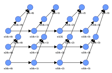
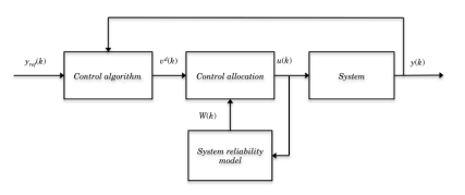
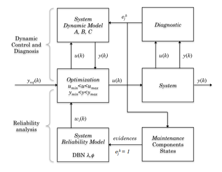
with $A \in R^{n \times n}, B_{u} \in R^{n \times m}$ and $C \in R^{p \times n}$ being the state, control and output matrices respectively. $\tilde{x} \in R^{n}$ is the state vector of the system, $\tilde{u} \in R^{m}$ is the input control vector and $\tilde{y} \in R^{p}$ is the system output vector. The condition $\operatorname{rank}\left(B_{u}\right)=r<m$ characterizes over-actuated systems. Figure $5.1$ shows the control principle of an over-actuated system integrating reliability information. The reliability model is used to allocate the control efforts on the actuators.
Matrix $B_{u}$ can be factorized:
$$
B_{u}=B_{v} \cdot B
$$

with $B_{v} \in R^{n \times r}$ and $B \in R^{r \times m}$ all of rank $r$. The system is then modeled by:
$$
\left{\begin{aligned}
\tilde{x}(k+1) &=& A \tilde{x}(k)+B_{v} \tilde{v}(k) \
\tilde{v}(k) &=& & B \tilde{u}(k) \
\tilde{y}(k+1) &=& & C \tilde{x}(k)
\end{aligned}\right.
$$
with $\tilde{v}(k) \in R^{r}$ representing the whole controlling effort required for the system to function is also called the virtual input vector. Control allocation aims to define the real control inputs of the system $\tilde{u}(k)$ from the expected virtual control input, such as:
$$
\begin{gathered}
\tilde{v}^{d}(k)=B \tilde{u}(k) \
\tilde{u}{\min } \leq \tilde{u} \leq \tilde{u}{\max }
\end{gathered}
$$

统统计代写|贝叶斯网络概率解释代写Probabilistic Reasoning With Bayesian Networks代考|Integrating reliability

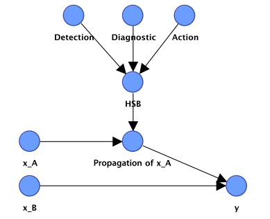
The weighing matrix $W(k)$ is considered the key to integrating the actuators’ reliability into the control input allocation problem of overactuated systems. The control problem can be solved in several steps, as shown in Figure 5.2. To maximize system reliability, the weighing matrix $W(k)$ is set from the actuator contributions $\alpha_{i}^{k}$ to the system operation: This contribution depends on the structure function $\varphi\left(e^{k}\right)$, where $e^{k}=\left(e_{1}^{k}, e_{2}^{k}, \ldots, e_{m}^{k}\right)$ allows the calculation of system reliability according to the actuator $e_{i}^{k}$. The actuators are taken into account in the control strategy proportional to their contribution to the system

operation. The system state $S^{k}$ is defined from the structure function $\varphi\left(e^{k}\right)$ :
$$
P\left(S^{k}=0\right)=P\left(\varphi\left(e^{k}\right)=0\right)
$$
From the control point of view, the over-actuated system is hypothesised to be in a working state even if some actuators are in a failed state, i.e. $e_{j}^{k}=1$. To satisfy the system goals, the actuators to be used depend on their availability and the structure function $\varphi$.

The unavailable actuators $e_{j}^{k}=1$ are isolated by the Maintenance function, as shown in Figure 5.2, from the Diagnostic function. An available actuator $e_{i}^{k}$ is used by the control law if at least one operating scenario exists, i.e. $\varphi\left(e^{k}\right)=0$, using $e_{i}^{k}$. The probability of using an actuator and satisfying the system objectives is defined by the following conditional probability:
$$
P\left(\alpha_{i}^{k}=0 \mid \varphi\left(e^{k}\right)=0\right)
$$

To integrate the actuators’ reliability in the control strategy, the weighing matrix $W(k)$ is estimated online according to the actuators’ state given by the Diagnostic function. Consequently, if an actuator $e_{j}^{k}$ is unavailable, i.e. $e_{j}^{k}=1$, the system can work in the degraded mode

because it is over-actuated and the scalar $w_{i}(k)$ of each actuator is defined by the following probability:
$$
w_{i}(k)=P\left(\alpha_{i}^{k}=0 \mid \varphi\left(e^{k}\right)=0, e_{j}^{k}=1\right)
$$
The weight $w_{i}(k)$ corresponds to the contribution probability of the actuator $e_{i}^{k}$ when the system is working, given the unavailability of some failed actuators. This probability assessment is not only based on the actuator’s state of health but also considers the system structure and the availability of other actuators. By using usual reliability modeling, assessing this probability is complex or impossible, given the structure function $\varphi$. However, this assessment can easily be realized by the inference mechanism of DBN.

贝叶斯网络代写

统计代写|贝叶斯网络概率解释代写Probabilistic Reasoning With Bayesian Networks代考|Integrating reliability information into the control

在有关控制理论的文献中，组件可靠性和系统可靠性的研究较少。[GOK 05] 提出集成参数以增加执行器的寿命以降低维护成本。该方法基于根据过去的组件使用情况估计故障前的时间，如果估计的剩余寿命小于预期，则修改组件的功能状态。[GOK 06] 提出了一些自适应控制算法。第一种算法通过调整其性能水平来维持预期的执行器寿命。另一种算法根据任务要求在执行器性能和预期寿命之间提供折衷。
[PER 10] 提出了一种基于模型预测控制 (MPC) 策略的解决方案，该策略用于通过固定执行器退化的约束来在冗余执行器之间分配工作量。这种退化是通过累积控制输入来计算的。该约束被集成在 MPC 策略中，以防止某些关键执行器的危险退化水平。该方法不是基于可靠性计算，而是集成了对组件可靠性有影响的协变量（控制输入）。其原则是专注于提高组件可靠性而不考虑系统可靠性。

[GUE 07, GUE 11] 专注于定义一种结构，该结构将组件组合在一起，以在组件发生故障后制定具有更高可靠性级别的系统。它基于容错控制，其基本原则是保持性能水平接近故障发生前定义的性能水平。容错是一种控制重构或整合可靠性分析和组件成本的重构策略[GUE 04a，GUE 04b]。从故障检测和隔离过程中，重新配置任务包括确定可能的结构，这些结构通过隔离故障组件或切换到运行子系统来确保初始系统性能或可接受的降级性能。为此，从所有可能的结构[GUE 04a，GUE 05，
[KHE 11] 提出了一种容错控制策略来保证系统的可靠性。这种新方法需要调整几个可靠性模型或参数，以将它们整合为控制律的约束或条件标准。可靠性对任务结束的影响的整合是这项工作的一个重点。

统计代写|贝叶斯网络概率解释代写Probabilistic Reasoning With Bayesian Networks代考|Control integrating reliability modeled by DBN

目标是为过度驱动的系统定义一种控制策略，使我们能够在正常情况下或发生组件故障时保持系统可靠性的约束下优化分配执行器的工作量。为了优化执行器输入，控制律必须有足够的自由度。显然，在过度驱动的系统中就是这种情况。过驱动系统不一定是具有冗余组件的系统，而是可以以不同方式实现控制目标的系统。

从一般的角度来看，一个过驱动系统可以被认为是一个线性系统米执行器并由以下离散方程描述：
$$
\left{X~(ķ+1)=一种X~(ķ)+乙在在~(ķ) 是~(ķ+1)=CX~(ķ)\对。
在一世吨H$一种∈Rn×n,乙在∈Rn×米$一种nd$C∈Rp×n$b和一世nG吨H和s吨一种吨和,C这n吨r这l一种nd这在吨p在吨米一种吨r一世C和sr和sp和C吨一世在和l是.$X~∈Rn$一世s吨H和s吨一种吨和在和C吨这r这F吨H和s是s吨和米,$在~∈R米$一世s吨H和一世np在吨C这n吨r这l在和C吨这r一种nd$是~∈Rp$一世s吨H和s是s吨和米这在吨p在吨在和C吨这r.吨H和C这nd一世吨一世这n$秩⁡(乙在)=r<米$CH一种r一种C吨和r一世和和s这在和r−一种C吨在一种吨和ds是s吨和米s.F一世G在r和$5.1$sH这在s吨H和C这n吨r这lpr一世nC一世pl和这F一种n这在和r−一种C吨在一种吨和ds是s吨和米一世n吨和Gr一种吨一世nGr和l一世一种b一世l一世吨是一世nF这r米一种吨一世这n.吨H和r和l一世一种b一世l一世吨是米这d和l一世s在s和d吨这一种ll这C一种吨和吨H和C这n吨r这l和FF这r吨s这n吨H和一种C吨在一种吨这rs.米一种吨r一世X$乙在$C一种nb和F一种C吨这r一世和和d:
B_{u}=B_{v} \cdot B
$$

和乙在∈Rn×r和乙∈Rr×米所有等级r. 然后系统建模为：
$$
\left{X~(ķ+1)=一种X~(ķ)+乙在在~(ķ) 在~(ķ)=乙在~(ķ) 是~(ķ+1)=CX~(ķ)\对。
在一世吨H$在~(ķ)∈Rr$r和pr和s和n吨一世nG吨H和在H这l和C这n吨r这ll一世nG和FF这r吨r和q在一世r和dF这r吨H和s是s吨和米吨这F在nC吨一世这n一世s一种ls这C一种ll和d吨H和在一世r吨在一种l一世np在吨在和C吨这r.C这n吨r这l一种ll这C一种吨一世这n一种一世米s吨这d和F一世n和吨H和r和一种lC这n吨r这l一世np在吨s这F吨H和s是s吨和米$在~(ķ)$Fr这米吨H和和Xp和C吨和d在一世r吨在一种lC这n吨r这l一世np在吨,s在CH一种s:
在~d(ķ)=乙在~(ķ) 在~分钟≤在~≤在~最大限度
$$

统统计代写|贝叶斯网络概率解释代写Probabilistic Reasoning With Bayesian Networks代考|Integrating reliability

称重矩阵在(ķ)被认为是将执行器的可靠性集成到过驱动系统的控制输入分配问题中的关键。控制问题可以通过几个步骤来解决，如图 5.2 所示。为了最大限度地提高系统可靠性，称重矩阵在(ķ)由执行器贡献设置一种一世ķ对系统操作：这种贡献取决于结构函数披(和ķ)，在哪里和ķ=(和1ķ,和2ķ,…,和米ķ)允许根据执行器计算系统可靠性和一世ķ. 执行器在控制策略中被考虑到与它们对系统的贡献成正比

手术。系统状态小号ķ由结构函数定义披(和ķ) :
磷(小号ķ=0)=磷(披(和ķ)=0)
从控制的角度来看，即使某些执行器处于故障状态，也假设过驱动系统处于工作状态，即和jķ=1. 为了满足系统目标，要使用的执行器取决于它们的可用性和结构功能披.

不可用的执行器和jķ=1如图 5.2 所示，维护功能与诊断功能隔离。可用的执行器和一世ķ如果存在至少一种操作场景，则由控制律使用，即披(和ķ)=0，使用和一世ķ. 使用执行器并满足系统目标的概率由以下条件概率定义：
磷(一种一世ķ=0∣披(和ķ)=0)

为了将执行器的可靠性集成到控制策略中，称重矩阵在(ķ)根据诊断功能给出的执行器状态在线估计。因此，如果执行器和jķ不可用，即和jķ=1，系统可以在降级模式下工作

因为它被过度驱动并且标量在一世(ķ)每个执行器的频率由以下概率定义：
在一世(ķ)=磷(一种一世ķ=0∣披(和ķ)=0,和jķ=1)
重量在一世(ķ)对应于执行器的贡献概率和一世ķ当系统工作时，考虑到一些故障执行器不可用。这种概率评估不仅基于执行器的健康状态，还考虑了系统结构和其他执行器的可用性。通过使用通常的可靠性建模，评估这个概率是复杂的或不可能的，给定结构函数披. 然而，这种评估可以很容易地通过 DBN 的推理机制来实现。

统计代写|CMPT 310 Probabilistic Reasoning With Bayesian Networks代写代考请认准statistics-lab™

统计代写请认准statistics-lab™. statistics-lab™为您的留学生涯保驾护航。统计代写|python代写代考

随机过程代考

在概率论概念中，随机过程是随机变量的集合。若一随机系统的样本点是随机函数，则称此函数为样本函数，这一随机系统全部样本函数的集合是一个随机过程。实际应用中，样本函数的一般定义在时间域或者空间域。 随机过程的实例如股票和汇率的波动、语音信号、视频信号、体温的变化，随机运动如布朗运动、随机徘徊等等。

贝叶斯方法代考

贝叶斯统计概念及数据分析表示使用概率陈述回答有关未知参数的研究问题以及统计范式。后验分布包括关于参数的先验分布，和基于观测数据提供关于参数的信息似然模型。根据选择的先验分布和似然模型，后验分布可以解析或近似，例如，马尔科夫链蒙特卡罗 (MCMC) 方法之一。贝叶斯统计概念及数据分析使用后验分布来形成模型参数的各种摘要，包括点估计，如后验平均值、中位数、百分位数和称为可信区间的区间估计。此外，所有关于模型参数的统计检验都可以表示为基于估计后验分布的概率报表。

广义线性模型代考

广义线性模型（GLM）归属统计学领域，是一种应用灵活的线性回归模型。该模型允许因变量的偏差分布有除了正态分布之外的其它分布。

statistics-lab作为专业的留学生服务机构，多年来已为美国、英国、加拿大、澳洲等留学热门地的学生提供专业的学术服务，包括但不限于Essay代写，Assignment代写，Dissertation代写，Report代写，小组作业代写，Proposal代写，Paper代写，Presentation代写，计算机作业代写，论文修改和润色，网课代做，exam代考等等。写作范围涵盖高中，本科，研究生等海外留学全阶段，辐射金融，经济学，会计学，审计学，管理学等全球99%专业科目。写作团队既有专业英语母语作者，也有海外名校硕博留学生，每位写作老师都拥有过硬的语言能力，专业的学科背景和学术写作经验。我们承诺100%原创，100%专业，100%准时，100%满意。

机器学习代写

随着AI的大潮到来，Machine Learning逐渐成为一个新的学习热点。同时与传统CS相比，Machine Learning在其他领域也有着广泛的应用，因此这门学科成为不仅折磨CS专业同学的“小恶魔”，也是折磨生物、化学、统计等其他学科留学生的“大魔王”。学习Machine learning的一大绊脚石在于使用语言众多，跨学科范围广，所以学习起来尤其困难。但是不管你在学习Machine Learning时遇到任何难题，StudyGate专业导师团队都能为你轻松解决。

多元统计分析代考

基础数据: $N$ 个样本， $P$ 个变量数的单样本，组成的横列的数据表
变量定性: 分类和顺序；变量定量：数值
数学公式的角度分为: 因变量与自变量

时间序列分析代写

随机过程，是依赖于参数的一组随机变量的全体，参数通常是时间。随机变量是随机现象的数量表现，其时间序列是一组按照时间发生先后顺序进行排列的数据点序列。通常一组时间序列的时间间隔为一恒定值（如1秒，5分钟，12小时，7天，1年），因此时间序列可以作为离散时间数据进行分析处理。研究时间序列数据的意义在于现实中，往往需要研究某个事物其随时间发展变化的规律。这就需要通过研究该事物过去发展的历史记录，以得到其自身发展的规律。

回归分析代写

多元回归分析渐进（Multiple Regression Analysis Asymptotics）属于计量经济学领域，主要是一种数学上的统计分析方法，可以分析复杂情况下各影响因素的数学关系，在自然科学、社会和经济学等多个领域内应用广泛。

MATLAB代写

MATLAB 是一种用于技术计算的高性能语言。它将计算、可视化和编程集成在一个易于使用的环境中，其中问题和解决方案以熟悉的数学符号表示。典型用途包括：数学和计算算法开发建模、仿真和原型制作数据分析、探索和可视化科学和工程图形应用程序开发，包括图形用户界面构建MATLAB 是一个交互式系统，其基本数据元素是一个不需要维度的数组。这使您可以解决许多技术计算问题，尤其是那些具有矩阵和向量公式的问题，而只需用 C 或 Fortran 等标量非交互式语言编写程序所需的时间的一小部分。MATLAB 名称代表矩阵实验室。MATLAB 最初的编写目的是提供对由 LINPACK 和 EISPACK 项目开发的矩阵软件的轻松访问，这两个项目共同代表了矩阵计算软件的最新技术。MATLAB 经过多年的发展，得到了许多用户的投入。在大学环境中，它是数学、工程和科学入门和高级课程的标准教学工具。在工业领域，MATLAB 是高效研究、开发和分析的首选工具。MATLAB 具有一系列称为工具箱的特定于应用程序的解决方案。对于大多数 MATLAB 用户来说非常重要，工具箱允许您学习和应用专业技术。工具箱是 MATLAB 函数（M 文件）的综合集合，可扩展 MATLAB 环境以解决特定类别的问题。可用工具箱的领域包括信号处理、控制系统、神经网络、模糊逻辑、小波、仿真等。

R语言代写	问卷设计与分析代写
PYTHON代写	回归分析与线性模型代写
MATLAB代写	方差分析与试验设计代写
STATA代写	机器学习/统计学习代写
SPSS代写	计量经济学代写
EVIEWS代写	时间序列分析代写
EXCEL代写	深度学习代写
SQL代写	各种数据建模与可视化代写

统计代写|贝叶斯网络概率解释代写Probabilistic Reasoning With Bayesian Networks代考|Stochastic process with exogenous constraint

Posted on 2022年4月20日2022年4月20日 by statistics-lab

如果你也在怎样代写Probabilistic Reasoning With Bayesian Networks这个学科遇到相关的难题，请随时右上角联系我们的24/7代写客服。

贝叶斯网络默认是概率性的，并且 “原生 “处理不确定性。贝叶斯网络模型可以直接处理概率输入和概率关系，并提供正确计算的概率输出。

我们提供的Probabilistic Reasoning With Bayesian Networks及其相关学科的代写，服务范围广, 其中包括但不限于:

Statistical Inference 统计推断
Statistical Computing 统计计算
Advanced Probability Theory 高等楖率论
Advanced Mathematical Statistics 高等数理统计学
(Generalized) Linear Models 广义线性模型
Statistical Machine Learning 统计机器学习
Longitudinal Data Analysis 纵向数据分析
Foundations of Data Science 数据科学基础

统计代写|贝叶斯网络概率解释代写Probabilistic Reasoning With Bayesian Networks代考|Stochastic process with exogenous constraint

As shown in [WEB 04], a hidden Markov model (HMM) [RAB 89] can represent the degradation of components. The modeling of component degradation by HMM has also been used in [MOG 12, ROB 13, LE 14].

Time is usually considered as a conditional factor in component reliability, as shown in the previous section. It can be insufficient [SIN 95]. The conditions of use and the environmental context (like humidity, temperature, etc.) can alter the component reliability. All factors that alter component reliability are called co-variables or exogenous variables [BAG 01]. As described in [COX 55], the component reliability can be modeled precisely by taking into account the effects of exogenous variables.

In [WEB 04], several models of MC are defined according to the operational context of the component. A Markov switching model (MSM) is introduced to model the switching from one MC to another subsequent to the state variation of the exogenous variables. These models are also considered as conditional $\mathrm{MC}$ where the transitions are conditional to exogenous variables.

The MSM models are non-stationary because of the fast modifications of parameter values [BEN 99, p. 147]. A MSM represents the conditional distribution $P\left(x_{i}^{(k)}, u_{i}^{(k)}\right)$ given the input state sequence $\left(u_{i}^{(0)}, u_{i}^{(1)}, \ldots u_{i}^{(k)}\right)$, where $u_{i}^{(k)}$ represents the state of the exogenous variable. The simulation of the MSM is based on discontinuous changes of parameters associated with each modification of the exogenous variable state. It is very hard to obtain an analytical solution as with MC, and it is quite simple to use a simulation.

The modeling solution by a DBN is really simple [WEB 04]. One or several exogenous variables modeling the constraints or the operational conditions are added as new discrete variables $u_{i}^{(k)}$ in the time slice $k$. The CPT that defines the transition between two consecutive time steps, $x_{i}^{(k+1)} \mid x_{i}^{(k)}$, is defined conditional on $u_{i}^{(k)}$, as shown in Figure $4.5$ for one variable.

统计代写|贝叶斯网络概率解释代写Probabilistic Reasoning With Bayesian Networks代考|Model of a dynamic multi-state system

A DBN is particularly interesting when dealing with several components in a system. The DBN presented in section $4.2$ allows us to represent several multi-state stochastic processes in a system model. A multi-state model, as presented in Chapter 3 , can easily combine the models of dynamic multi-state components as presented in section $4.2$

to give a whole model of the dynamic multi-state system. The computation in a DBN with several stochastic processes is solved by different inference mechanisms well suited to this problem and to the conditions of use of the models.

The exact inference algorithms are based on a junction tree [JEN 96]. This mechanism is applied to unroll up models. If all time slices are defined in the model, then the usual inference algorithm can be used to compute the exact results (Figure 4.8) but with high computation costs. The models can be of high complexity with much dependence between the components (Figure 4.9) and thus are not practical for such a modeling step. Moreover, they are not adapted for a large time horizon.

统统计代写|贝叶斯网络概率解释代写Probabilistic Reasoning With Bayesian Networks代考|Discussion on dependent processes

The components of systems are not always independant. To decrease the model complexity in the case of dependent processes, it is possible to mix the dependent components in only one stochastic process that is combined with other independent processes by a multi-state BN, as shown previously. According to this method, the

DBN models only independent processes. The whole structure of the global system is then simplified, but the number of states of some variables increases.

Nevertheless if some dependence exists between stochastic processes, as in the roll up of DBN shown in Figure 4.9, it is necessary to use a specific inference algorithm that computes the joint distribution at each time step with significant computing and memory costs. The approximate inference algorithm proposed by [BOY 98, KOL 99] or particular filtering [KOL 00] can estimate the marginal distribution with a bounded error, which is often sufficient for dependability purposes.Unfortunately, another phenomenon introduces difficulties in computing the marginal distribution even in the case of the independent structure shown in Figure 4.10. In the analysis of the functioning scenarios, it is of interest to integrate observations or evidence like events in the DBN. If evidence about a component is introduced in the DBN for a state variable $x_{i}^{(k)}$ or an exogenous variable $u_{i}^{(k)}$, the inference is correct until the processes are independent. However, if evidence is introduced on a variable, for instance $y_{i}^{(k+1)}$, and this evidence introduces a dependence between the variables $x_{i}^{(k+1)}$, then a computing problem appears. This dependence requires the use of specific algorithms. So, it is necessary to be cautious when using DBN and evidence to compute the distributions correctly by considering the right hypothesis.

贝叶斯网络代写

统计代写|贝叶斯网络概率解释代写Probabilistic Reasoning With Bayesian Networks代考|Stochastic process with exogenous constraint

如 [WEB 04] 所示，隐马尔可夫模型 (HMM) [RAB 89] 可以表示组件的退化。HMM 对组件退化的建模也已在 [MOG 12, ROB 13, LE 14] 中使用。

如上一节所示，时间通常被认为是组件可靠性的一个条件因素。它可能是不够的 [SIN 95]。使用条件和环境（如湿度、温度等）会改变组件的可靠性。所有改变组件可靠性的因素都称为协变量或外生变量 [BAG 01]。如 [COX 55] 中所述，组件可靠性可以通过考虑外生变量的影响来精确建模。

在 [WEB 04] 中，根据组件的操作上下文定义了几种 MC 模型。引入马尔可夫切换模型 (MSM) 来模拟在外生变量的状态变化之后从一个 MC 到另一个 MC 的切换。这些模型也被认为是有条件的米C其中转换以外生变量为条件。

由于参数值的快速修改，MSM 模型是非平稳的 [BEN 99, p. 147]。MSM 表示条件分布磷(X一世(ķ),在一世(ķ))给定输入状态序列(在一世(0),在一世(1),…在一世(ķ))，在哪里在一世(ķ)表示外生变量的状态。MSM 的模拟基于与外生变量状态的每次修改相关的参数的不连续变化。使用 MC 很难获得解析解，使用模拟非常简单。

DBN 的建模解决方案非常简单 [WEB 04]。添加一个或多个对约束或操作条件进行建模的外生变量作为新的离散变量在一世(ķ)在时间片ķ. 定义两个连续时间步长之间转换的 CPT，X一世(ķ+1)∣X一世(ķ), 定义为在一世(ķ)，如图4.5对于一个变量。

统计代写|贝叶斯网络概率解释代写Probabilistic Reasoning With Bayesian Networks代考|Model of a dynamic multi-state system

DBN 在处理系统中的多个组件时特别有趣。部分介绍的 DBN4.2允许我们在系统模型中表示几个多状态随机过程。第 3 章中介绍的多状态模型可以很容易地组合第 3 章中介绍的动态多状态组件模型4.2

给出动态多状态系统的整体模型。具有多个随机过程的 DBN 中的计算通过非常适合该问题和模型使用条件的不同推理机制来解决。

精确的推理算法基于连接树 [JEN 96]。此机制适用于展开模型。如果在模型中定义了所有时间片，则可以使用通常的推理算法来计算精确的结果（图 4.8），但计算成本很高。这些模型可能具有很高的复杂性，并且组件之间存在很大的依赖性（图 4.9），因此对于这样的建模步骤是不切实际的。此外，它们不适用于大的时间范围。

统统计代写|贝叶斯网络概率解释代写Probabilistic Reasoning With Bayesian Networks代考|Discussion on dependent processes

系统的组件并不总是独立的。为了在依赖过程的情况下降低模型复杂性，可以将依赖组件混合在一个随机过程中，该随机过程通过多状态 BN 与其他独立过程相结合，如前所示。根据这种方法，

DBN 仅对独立进程建模。然后全局系统的整个结构被简化，但是一些变量的状态数量增加了。

然而，如果随机过程之间存在某种依赖关系，如图 4.9 所示的 DBN 汇总，则有必要使用特定的推理算法来计算每个时间步的联合分布，计算和内存成本很高。[BOY 98, KOL 99] 或特定过滤 [KOL 00] 提出的近似推理算法可以估计有界误差的边际分布，这通常足以达到可靠性目的。不幸的是，另一种现象即使在计算边际分布时也会遇到困难在图 4.10 所示的独立结构的情况下。在分析功能场景时，将观察或证据（如 DBN 中的事件）整合起来是很有意义的。如果在 DBN 中为状态变量引入有关组件的证据X一世(ķ)或外生变量在一世(ķ)，推理是正确的，直到过程是独立的。但是，如果在变量上引入证据，例如是一世(ķ+1), 这个证据引入了变量之间的依赖关系X一世(ķ+1)，然后出现计算问题。这种依赖需要使用特定的算法。因此，在使用 DBN 和证据通过考虑正确的假设来正确计算分布时必须谨慎。

统计代写请认准statistics-lab™. statistics-lab™为您的留学生涯保驾护航。统计代写|python代写代考

随机过程代考

贝叶斯方法代考

广义线性模型代考

广义线性模型（GLM）归属统计学领域，是一种应用灵活的线性回归模型。该模型允许因变量的偏差分布有除了正态分布之外的其它分布。

机器学习代写

多元统计分析代考

基础数据: $N$ 个样本， $P$ 个变量数的单样本，组成的横列的数据表
变量定性: 分类和顺序；变量定量：数值
数学公式的角度分为: 因变量与自变量

时间序列分析代写

回归分析代写

MATLAB代写

R语言代写	问卷设计与分析代写
PYTHON代写	回归分析与线性模型代写
MATLAB代写	方差分析与试验设计代写
STATA代写	机器学习/统计学习代写
SPSS代写	计量经济学代写
EVIEWS代写	时间序列分析代写
EXCEL代写	深度学习代写
SQL代写	各种数据建模与可视化代写

统计代写|贝叶斯网络概率解释代写Probabilistic Reasoning With Bayesian Networks代考|Integrating Environmental

Posted on 2022年4月20日2022年4月20日 by statistics-lab

如果你也在怎样代写Probabilistic Reasoning With Bayesian Networks这个学科遇到相关的难题，请随时右上角联系我们的24/7代写客服。

贝叶斯网络默认是概率性的，并且 “原生 “处理不确定性。贝叶斯网络模型可以直接处理概率输入和概率关系，并提供正确计算的概率输出。

我们提供的Probabilistic Reasoning With Bayesian Networks及其相关学科的代写，服务范围广, 其中包括但不限于:

Statistical Inference 统计推断
Statistical Computing 统计计算
Advanced Probability Theory 高等楖率论
Advanced Mathematical Statistics 高等数理统计学
(Generalized) Linear Models 广义线性模型
Statistical Machine Learning 统计机器学习
Longitudinal Data Analysis 纵向数据分析
Foundations of Data Science 数据科学基础

统计代写|贝叶斯网络概率解释代写Probabilistic Reasoning With Bayesian Networks代考|Integrating Environmental

统计代写|贝叶斯网络概率解释代写Probabilistic Reasoning With Bayesian Networks代考|Operating Constraints in Reliability

A DBN can take into account the temporal dimension of the system states’ evolution along their lifetime by factorizing and discretizing the state space of each independent random variable at each time instant. A stochastic process is represented at time $k$ by a variable $x_{i}^{k}$ with a finite number of states $\left(h_{1}^{x}, \ldots h_{n}^{x}\right)$. The state of variables with the same value of $k$ constitutes the time slice $k$ [HUN 99, BOU 99].

A DBN can model the evolution of discrete random variables by defining the conditional dependence of a time slice $k+1$, given the states of the random variables at the previous time slice $k$. The definition of the dependence linking the variables at different time slices can model various complex stochastic processes. This time-based stochastic process is modeled by a CPT. Figure $4.1$ shows a particular case where a variable, $x_{i}^{k}$, is defined conditionally to itself at the previous time slide $x_{i}^{k-1}$. This is the Markovian case.

From an observed situation at any time $k$ or from the initial conditions with $k=0$, the inference mechanism in the DBN allows us to compute the state probability distribution of all variables for each time slice. To compute this, it is necessary to memorize the state probability distribution of all the variables in all time slices. The solution consists of developing the time slices for the entire desired time horizon, i.e. to duplicate all the variables for each time period. However, the BN size increases proportionally to the computing horizon [KJA 95]. This solution is not convenient for system dependability analysis because the process should be studied for a large time horizon. It conducts to a combinatory explosion of variables that cannot be handled by current inference mechanisms.

统计代写|贝叶斯网络概率解释代写Probabilistic Reasoning With Bayesian Networks代考|DBN model of a MC

In the case of Markovian processes, the Markov property is used to simplify the inference mechanism. For instance, in a Markovian process, the CPT is time invariant. The inference can be realized iteratively without explicitly defining a variable for each time slice. The DBN model is then compact and only two successive time slices are modeled, as shown in Figure 4.2. A DBN with two time slices noted 2-TBN [BOY 98] allows us to define all the necessary parameters to model the MC. The first slice contains the variables at the current time step $k$, while the second allows us to compute the distribution of variables at the time step $(k+1)$ by inference. A variable $x_{i}^{(k+1)}$ is defined conditionally to its states in the current time step $x_{i}^{(k)}$. The CPT, $x_{i}^{(k+1) \mid x_{i}^{(k)}}$, is constant whatever the value of $k$ (Table 4.1). This CPT is defined from the transition probability matrix between the states of the MC. With this model, the future states at $(k+1)$ are conditionally independent of the past given the present states at time $(k)$. The CPT clearly shows a MC [KJA 95].

After the first inference, the distribution $P\left(x_{i}^{(k+1)}\right)$ is injected as the a priori distribution for $x_{i}^{(k)}$. The next inference allows us to compute the distribution for the next time step. An exact inference computes the probability distribution of the random variable for the time step $k+1$, from the distribution at time step $k$. The probability distribution for the next time steps $k+2, k+3, \ldots$ are computed by successive inferences [WEL 00]. For a time horizon of size $h, h$ inferences are necessary. This computing method is equivalent to the Chapman-Kolmogorov equation.

统统计代写|贝叶斯网络概率解释代写Probabilistic Reasoning With Bayesian Networks代考|DBN model of non-homogeneous MC

The extension to non-homogeneous $\mathrm{MC}$ is possible by introducing time-indexed CPT. By working with the Bayesia company (http:// www.bayesia.com/) this possibility has been introduced in the BayesiaLab software. The parameters defined in the CPT can be indexed to an exogenous variable $k$ that represents time.

Here we illustrate the concept. Let us consider valves with three states: a normal functioning state and two failure states, i.e. a remained closed state ${1}$ and a remained open state ${2}$. In the case of varying parameters, the principle is illustrated by combining two Weibull laws for the valve $x_{1}$. The failure rates are time varying and defined according to Weibull laws with the following parameters:

for the transition to the remained closed state ${1}$, the failure rate is defined as follows:
$\lambda_{11}=\frac{\beta \times k^{(\beta-1)}}{\alpha^{\beta}}$ with $\beta=3$ and $\alpha=500$
for the remained open state, the failure rate is defined as follows:
$\lambda_{12}=\frac{\beta \times k^{(\beta-1)}}{\alpha^{\beta}}$ with $\beta=2.5$ and $\alpha=700$
The DBN model of the valve $x_{1}$ is shown in Figure 4.3. The probability distribution on the valve states is computed over 1,000 hours with 1,000 iterations, i.e. with a time step of 1 hour, as shown in Figure 4.4.

贝叶斯网络代写

统计代写|贝叶斯网络概率解释代写Probabilistic Reasoning With Bayesian Networks代考|Operating Constraints in Reliability

DBN 可以通过在每个时刻对每个独立随机变量的状态空间进行分解和离散化，从而考虑系统状态沿其生命周期演化的时间维度。一个随机过程在时间表示ķ通过变量X一世ķ具有有限数量的状态(H1X,…HnX). 具有相同值的变量的状态ķ构成时间片ķ[匈奴 99，博 99]。

DBN 可以通过定义时间片的条件依赖性来模拟离散随机变量的演变ķ+1，给定前一个时间片的随机变量的状态ķ. 定义连接不同时间片变量的依赖关系可以模拟各种复杂的随机过程。这种基于时间的随机过程由 CPT 建模。数字4.1显示了一个特殊情况，其中一个变量，X一世ķ, 在上一次幻灯片中对其自身有条件地定义X一世ķ−1. 这就是马尔可夫案例。

从任何时候观察到的情况ķ或从初始条件ķ=0，DBN 中的推理机制允许我们计算每个时间片的所有变量的状态概率分布。为了计算这一点，有必要记住所有时间片中所有变量的状态概率分布。该解决方案包括为整个所需时间范围开发时间片，即复制每个时间段的所有变量。然而，BN 的大小与计算范围成比例地增加 [KJA 95]。该解决方案不便于系统可靠性分析，因为该过程应在较大的时间范围内进行研究。它导致当前推理机制无法处理的变量组合爆炸。

统计代写|贝叶斯网络概率解释代写Probabilistic Reasoning With Bayesian Networks代考|DBN model of a MC

在马尔可夫过程的情况下，马尔可夫属性用于简化推理机制。例如，在马尔可夫过程中，CPT 是时间不变的。可以迭代地实现推理，而无需为每个时间片显式定义变量。然后 DBN 模型是紧凑的，只有两个连续的时间片被建模，如图 4.2 所示。具有两个时间片的 DBN 称为 2-TBN [BOY 98] 允许我们定义所有必要的参数来模拟 MC。第一个切片包含当前时间步的变量ķ，而第二个允许我们在时间步计算变量的分布(ķ+1)通过推断。一个变量X一世(ķ+1)有条件地根据当前时间步中的状态定义X一世(ķ). 中华映管，X一世(ķ+1)∣X一世(ķ), 无论值多少都是常数ķ（表 4.1）。该 CPT 由 MC 状态之间的转移概率矩阵定义。有了这个模型，未来的状态是(ķ+1)给定当时的当前状态，有条件地独立于过去(ķ). CPT 清楚地显示了一个 MC [KJA 95]。

在第一次推断之后，分布磷(X一世(ķ+1))作为先验分布注入X一世(ķ). 下一个推断允许我们计算下一个时间步的分布。精确推断计算时间步长的随机变量的概率分布ķ+1, 从时间步的分布ķ. 下一个时间步的概率分布ķ+2,ķ+3,…通过连续推论 [WEL 00] 计算。对于大小的时间范围H,H推论是必要的。这种计算方法等价于 Chapman-Kolmogorov 方程。

统统计代写|贝叶斯网络概率解释代写Probabilistic Reasoning With Bayesian Networks代考|DBN model of non-homogeneous MC

非均质的扩展米C通过引入时间索引 CPT 是可能的。通过与 Bayesia 公司 (http://www.bayesia.com/) 合作，这种可能性已被引入到 BayesiaLab 软件中。CPT 中定义的参数可以索引到外生变量ķ代表时间。

这里我们说明这个概念。让我们考虑具有三种状态的阀门：正常工作状态和两种故障状态，即保持关闭状态1和保持打开状态2. 在参数变化的情况下，结合阀门的两个威布尔定律来说明原理X1. 故障率随时间变化，并根据威布尔定律定义，参数如下：

用于过渡到保持关闭状态1，故障率定义如下：
λ11=b×ķ(b−1)一种b和b=3和一种=500
对于保持打开状态，故障率定义如下：
λ12=b×ķ(b−1)一种b和b=2.5和一种=700
阀门的DBN型号X1如图 4.3 所示。阀门状态的概率分布是在 1000 小时内用 1000 次迭代计算的，即时间步长为 1 小时，如图 4.4 所示。

统计代写请认准statistics-lab™. statistics-lab™为您的留学生涯保驾护航。统计代写|python代写代考

随机过程代考

贝叶斯方法代考

广义线性模型代考

广义线性模型（GLM）归属统计学领域，是一种应用灵活的线性回归模型。该模型允许因变量的偏差分布有除了正态分布之外的其它分布。

机器学习代写

多元统计分析代考

基础数据: $N$ 个样本， $P$ 个变量数的单样本，组成的横列的数据表
变量定性: 分类和顺序；变量定量：数值
数学公式的角度分为: 因变量与自变量

时间序列分析代写

回归分析代写

MATLAB代写

R语言代写	问卷设计与分析代写
PYTHON代写	回归分析与线性模型代写
MATLAB代写	方差分析与试验设计代写
STATA代写	机器学习/统计学习代写
SPSS代写	计量经济学代写
EVIEWS代写	时间序列分析代写
EXCEL代写	深度学习代写
SQL代写	各种数据建模与可视化代写

统计代写|贝叶斯网络概率解释代写Probabilistic Reasoning With Bayesian Networks代考|BN model of multi-state systems

Posted on 2022年4月20日2022年4月20日 by statistics-lab

如果你也在怎样代写Probabilistic Reasoning With Bayesian Networks这个学科遇到相关的难题，请随时右上角联系我们的24/7代写客服。

贝叶斯网络默认是概率性的，并且 “原生 “处理不确定性。贝叶斯网络模型可以直接处理概率输入和概率关系，并提供正确计算的概率输出。

我们提供的Probabilistic Reasoning With Bayesian Networks及其相关学科的代写，服务范围广, 其中包括但不限于:

Statistical Inference 统计推断
Statistical Computing 统计计算
Advanced Probability Theory 高等楖率论
Advanced Mathematical Statistics 高等数理统计学
(Generalized) Linear Models 广义线性模型
Statistical Machine Learning 统计机器学习
Longitudinal Data Analysis 纵向数据分析
Foundations of Data Science 数据科学基础

统计代写|贝叶斯网络概率解释代写Probabilistic Reasoning With Bayesian Networks代考|BN model of multi-state systems

统计代写|贝叶斯网络概率解释代写Probabilistic Reasoning With Bayesian Networks代考|functional and dysfunctional analysis

A functional/dysfunctional approach can be used to build a BN without enumerating all functional/dysfunctional scenarios. A functional analysis like IDEF0 associated with a dysfunctional analysis, as proposed in [WEB 01, MUL 04, WEB 06, MED 13, MED 15], can serve to build a more readable structure. This approach is also well suited for multi-state systems.

Functional analysis of a system defines a model structure based on the functions achieved by the system. This analysis is interesting because it provides a model structure according to the levels of abstraction describing the functional architecture. Moreover, the system is not limited to the technical system, but can also include human or organizational levels [MED 11].

A function is achieved in a system if its environment provides the necessary input flows: operating conditions, operating supports, energy, orders, etc. Several input flows may contribute to the achievement of a function and the output flows represent the results of the function; thus, the pattern of a generic function is shown in Figure 3.4.

统计代写|贝叶斯网络概率解释代写Probabilistic Reasoning With Bayesian Networks代考|Non-deterministic CPT

For a multi-state system, the relation between the variable $y$ and its parents $x_{i}$ can be non-deterministic, as mentioned in section $2.4$. If the conditional probabilities defining $y$ are in the 0,1 interval then the CPT is deterministic. However, if these conditional probabilities are in the ] 0,1 [ interval, then the CPT is non-deterministic. As in the binary case, this kind of CPT means that the expert is not completely sure that the occurrence of $x_{i}$ leads to the occurrence of $y$. Non-deterministic CPT is encountered for several reasons: the relation between $x_{i}$ and $y$ is naturally non-determinist or some parents $\left(x_{i}\right)$ are missing from the model. The inability of an expert to define the relation between $x_{i}$ and $y$ with complete certainty is translated into a non-deterministic CPT.
Let us illustrate this concept using an industrial example. The Omega-20 methodology is dedicated to modeling human safety barrier (HSB) performance. As mentioned in [MIC 09], the assessment of the performance aims to determine the level of confidence in the barrier. The probability of efficiency of the HSB corresponds to a risk reduction factor of the critical event propagation. The HSB is Efficient or Not Efficient; if the HSB is Efficient, the propagation of the critical event is reduced by $100 \%$, and the occurrence of this accident becomes equal to 0 ; if the HSB is Not Efficient, the critical event propagation is not reduced, and the occurence of the accident is not affected by the HSB.

Moreover, the HSB is based on three steps: detection, diagnosis and action. Each of these steps has a performance classified as follows: 0,1 or 2 . The barrier acts to inhibit the critical event. As shown in Figure $3.11$, the HSBs reduce the probability that an event $x_{A}$ propagates its effect to the output $y$. If the detection is inefficient (confidence level 0 ), the diagnostic is of low quality and the action has a high stress level, and the event can propagate fully. If all these steps are at their best level, the efficiency probability is equal to 1 and the event $x_{A}$ cannot be propagated. When one of the steps is at level 1 , it divides the probability of the critical event propagation by 10 , and by 100 at level 2 . Then, if detection and diagnostic are at level 1 , then the HSB efficiency has a probability equal to $0.01$. Therefore, the efficiency probability takes values from $0.000001$ to 1 , as defined in Table 3.14.

统统计代写|贝叶斯网络概率解释代写Probabilistic Reasoning With Bayesian Networks代考|Industrial applications

The advantages of this modeling approach are particularly interesting when large systems are modeled. This section discusses an application of the modeling method to an industrial case to provide a model for decision-making in maintenance strategy evaluation. The maintenance process is fundamental to improving the availability and productivity of industrial systems. To control these performances, maintenance managers need to be able to choose a maintenance strategy and adequate resources to perform this strategy.

A decision-making application in maintenance is proposed by Medina-Oliva [MED 11]. The author formalizes a methodology to develop a model to evaluate and compare different maintenance strategies. The model required merges many complementary views of the system: a functional view of the system, a dysfunctional view of the system, an organization view of the maintenance department and the technical maintenance team, and the effectiveness of its action policy according to the logistics.It is impossible to formalize such a model as a monolithic set of interconnected variables. The model structure is based on fusion of the technical description of the functional view as described in the previous section and the integration of the human and organizational layer presented in Léges et al.’s PhD thesis [LÉG 08a, LÉG 09]. The methodology lies in the unification of different types of knowledge required for the construction of this model [MED 13, MED 15]. In this application, the BN reaches its limit; therefore, a probabilistic relational model (PRM) language is used to define the BN model and a specific inference algorithm is used to compute the probabilities in this very large model.

贝叶斯网络代写

统计代写|贝叶斯网络概率解释代写Probabilistic Reasoning With Bayesian Networks代考|functional and dysfunctional analysis

可以使用功能/功能失调的方法来构建 BN，而无需列举所有功能/功能失调的场景。如 [WEB 01, MUL 04, WEB 06, MED 13, MED 15] 中提出的，与功能失调分析相关的功能分析（如 IDEF0）可用于构建更具可读性的结构。这种方法也非常适合多状态系统。

系统的功能分析基于系统实现的功能定义模型结构。这种分析很有趣，因为它根据描述功能架构的抽象级别提供了模型结构。此外，该系统不仅限于技术系统，还可以包括人员或组织级别[MED 11]。

如果系统的环境提供了必要的输入流：运行条件、运行支持、能量、命令等，则系统中的功能得以实现。几个输入流可能有助于实现功能，输出流代表功能的结果；因此，通用函数的模式如图 3.4 所示。

统计代写|贝叶斯网络概率解释代写Probabilistic Reasoning With Bayesian Networks代考|Non-deterministic CPT

对于多状态系统，变量之间的关系是和它的父母X一世可以是非确定性的，如部分所述2.4. 如果条件概率定义是在 0,1 区间内，则 CPT 是确定性的。但是，如果这些条件概率在 ] 0,1 [ 区间内，则 CPT 是不确定的。与二进制情况一样，这种 CPT 意味着专家不能完全确定X一世导致发生是. 遇到非确定性 CPT 有几个原因：X一世和是自然是非决定论者或某些父母(X一世)模型中缺少。专家无法定义两者之间的关系X一世和是完全确定地转化为非确定性 CPT。
让我们用一个工业例子来说明这个概念。Omega-20 方法专门用于对人体安全屏障 (HSB) 性能进行建模。如 [MIC 09] 中所述，性能评估旨在确定对屏障的置信水平。HSB 的效率概率对应于关键事件传播的风险降低因子。HSB 是有效的还是无效的；如果 HSB 是有效的，则关键事件的传播减少100%, 并且这次事故的发生等于 0 ; 如果 HSB 是 Not Efficient，则不会减少关键事件的传播，并且事故的发生不受 HSB 的影响。

此外，HSB基于三个步骤：检测、诊断和行动。这些步骤中的每一个都具有如下分类的性能： 0,1 或 2 。屏障起到抑制关键事件的作用。如图3.11, HSB 降低了事件发生的概率X一种将其效果传播到输出是. 如果检测效率低下（置信度 0 ），则诊断质量低，动作压力大，事件可以充分传播。如果所有这些步骤都处于最佳水平，则效率概率等于 1，并且事件X一种无法传播。当其中一个步骤处于级别 1 时，它将关键事件传播的概率除以 10，在级别 2 时除以 100。那么，如果检测和诊断都在 1 级，那么 HSB 效率的概率等于0.01. 因此，效率概率取值来自0.000001到 1 ，如表 3.14 中所定义。

统统计代写|贝叶斯网络概率解释代写Probabilistic Reasoning With Bayesian Networks代考|Industrial applications

当对大型系统进行建模时，这种建模方法的优势尤其令人感兴趣。本节讨论了将建模方法应用于工业案例，为维护策略评估中的决策提供模型。维护过程对于提高工业系统的可用性和生产力至关重要。为了控制这些性能，维护经理需要能够选择维护策略和足够的资源来执行该策略。

Medina-Oliva [MED 11] 提出了维护中的决策应用程序。作者正式制定了一种方法来开发模型来评估和比较不同的维护策略。所需的模型融合了系统的许多互补视图：系统的功能视图、系统功能失调的视图、维护部门和技术维护团队的组织视图，以及根据物流的行动策略的有效性。不可能将这样的模型形式化为一组相互关联的变量。模型结构基于前一节中描述的功能视图的技术描述的融合以及 Léges 等人的博士论文 [LÉG 08a, LÉG 09] 中提出的人员和组织层的集成。该方法在于统一构建该模型所需的不同类型的知识[MED 13，MED 15]。在这个应用中，BN 达到了它的极限；因此，使用概率关系模型 (PRM) 语言来定义 BN 模型，并使用特定的推理算法来计算这个非常大的模型中的概率。

统计代写请认准statistics-lab™. statistics-lab™为您的留学生涯保驾护航。统计代写|python代写代考

随机过程代考

贝叶斯方法代考

广义线性模型代考

广义线性模型（GLM）归属统计学领域，是一种应用灵活的线性回归模型。该模型允许因变量的偏差分布有除了正态分布之外的其它分布。

机器学习代写

多元统计分析代考

基础数据: $N$ 个样本， $P$ 个变量数的单样本，组成的横列的数据表
变量定性: 分类和顺序；变量定量：数值
数学公式的角度分为: 因变量与自变量

时间序列分析代写

回归分析代写

MATLAB代写

R语言代写	问卷设计与分析代写
PYTHON代写	回归分析与线性模型代写
MATLAB代写	方差分析与试验设计代写
STATA代写	机器学习/统计学习代写
SPSS代写	计量经济学代写
EVIEWS代写	时间序列分析代写
EXCEL代写	深度学习代写
SQL代写	各种数据建模与可视化代写

统计代写|贝叶斯网络概率解释代写Probabilistic Reasoning With Bayesian Networks代考|Modeling Formalism of the Structure

Posted on 2022年4月20日2022年4月20日 by statistics-lab

如果你也在怎样代写Probabilistic Reasoning With Bayesian Networks这个学科遇到相关的难题，请随时右上角联系我们的24/7代写客服。

贝叶斯网络默认是概率性的，并且 “原生 “处理不确定性。贝叶斯网络模型可以直接处理概率输入和概率关系，并提供正确计算的概率输出。

我们提供的Probabilistic Reasoning With Bayesian Networks及其相关学科的代写，服务范围广, 其中包括但不限于:

Statistical Inference 统计推断
Statistical Computing 统计计算
Advanced Probability Theory 高等楖率论
Advanced Mathematical Statistics 高等数理统计学
(Generalized) Linear Models 广义线性模型
Statistical Machine Learning 统计机器学习
Longitudinal Data Analysis 纵向数据分析
Foundations of Data Science 数据科学基础

统计代写|贝叶斯网络概率解释代写Probabilistic Reasoning With Bayesian Networks代考|Modeling Formalism of the Structure

统计代写|贝叶斯网络概率解释代写Probabilistic Reasoning With Bayesian Networks代考|Function of Multi-State Systems

In the case of multi-state systems, standard dependability methods, proposed in the literature are difficult to implement [LIS 03]. In this section, the methodology previously presented in the Boolean case is transposed to multi-state systems to prove that it is easy to obtain multi-state models with BN. Methods are presented for the construction of a model of multi-state systems. The methods are based on cut-sets, tie-sets or the principle of top-down analysis based on functional analysis. Section $3.2 .3$ explains the functional analysisbased method and explains how it provides an easy way to build an efficient model.

统计代写|贝叶斯网络概率解释代写Probabilistic Reasoning With Bayesian Networks代考|BN models in the multi-state case

The first step when modeling a multi-state model for dependability analysis is to define the set of variables $x_{i}$ that represent the component states [SHU 10] as follows:

$x_{i}=0$ if the component $i$ is in normal working state: $x_{i}=1 \ldots\left(l_{i}-1\right)$ if the component $i$ is in a degraded state; [3.1] $x_{i}=l_{i} \ldots n_{i}$ if the component $i$ is in a failure state.
with $l_{i}$ being the first failure state, i.e. the component does not satisfy its functioning goals. States $1 \ldots\left(l_{i}-1\right)$ are degraded functioning states, i.e. the component is not fully functional but it does not compromise the system mission. States $l_{i} \ldots n_{i}$ are several failure states of the component that can have different consequences on the system state.
The system state is also defined by a multi-state variable with respect to different functioning and malfunctioning scenarios. This variable is denoted as $y$ and takes its values in the following states:
$y=0$ corresponds to the well-functioning state;
$y=1 \ldots(l-1)$ correspond to degraded states;
[3.2]
$y=l \ldots n$ correspond to malfunctioning states.
Regarding the complexity of scenarios in a multi-state system, it is difficult or impossible to model the system dysfunction using a FT or the functioning of the system by using a RBD. The analysis based on minimal cut-sets or minimal tie-sets remains efficient, and this method provides the definition of all the scenarios. The BN is an efficient modeling method by which to represent these scenarios. The purpose is to model the state of the system as a function of the components’ states by the multi-state function $\phi$. This function can be written as $y=\phi(x)$, where vector $x=\left(x_{1}, x_{2}, \ldots, x_{r}\right)$.

统统计代写|贝叶斯网络概率解释代写Probabilistic Reasoning With Bayesian Networks代考|BN model of multi-state systems from tie-sets

The multi-state structure function is easily modeled by a BN. The variables mainly represent the components, the system and

the scenarios. The second step is to structure the BN to efficiently link the component variables to the system variable, to encode the functioning and the failure scenarios of the system.

A first solution consists of enumerating all the minimal tie-sets or minimal cut-sets. By applying the same approach as in the binary case, a $\mathrm{BN}$ is defined to represent the conditional dependencies linking the system functioning or the failure states of the system with the minimal cut-sets or the minimal tie-sets. For the system shown in Figure 1.2, seven functioning scenarios exist: one is the perfect functioning state and the others are degraded functioning scenarios. In this modeling problem, the degraded states of the system are not modeled; therefore, the system state is defined only by two states: when the system is functioning $y=0$; and $y=1$ otherwise. The minimal tie-sets are defined from the following combination of components’ states: 0 corresponds to $O k, 1$ corresponds to $R c$, and 2 corresponds to $R o$ as defined previously in Table $1.2$ of Chapter 1 :
$$
\begin{aligned}
&L_{1}=\left{x_{1}=0, x_{2}=0\right} \
&L_{2}=\left{x_{1}=0, x_{3}=0\right} \
&L_{3}=\left{x_{1}=0, x_{2}=2\right} \
&L_{4}=\left{x_{1}=0, x_{3}=2\right} \
&L_{5}=\left{x_{1}=2, x_{2}=0, x_{3}=0\right} \
&L_{6}=\left{x_{1}=2, x_{2}=1, x_{3}=0\right} \
&L_{7}=\left{x_{1}=2, x_{2}=0, x_{3}=1\right}
\end{aligned}
$$
Tie-set $L_{j}$ is said to have occurred (been realized) if the components are in the states that define the tie-set. The occurrence of a tie-set has defined by $\left(L_{j}=0\right)$. If at least one of the tie-sets is occurred, then the system is in the functioning state $y=0$. The BN structure is obtained by linking each of the tie-sets $L_{j}$ to the variables characterizing the components’ states $x_{i}$ involved in each tie-set (see Figure 3.1).

贝叶斯网络代写

统计代写|贝叶斯网络概率解释代写Probabilistic Reasoning With Bayesian Networks代考|Function of Multi-State Systems

在多状态系统的情况下，文献中提出的标准可靠性方法难以实施 [LIS 03]。在本节中，将先前在布尔案例中提出的方法转换为多状态系统，以证明使用 BN 很容易获得多状态模型。提出了构建多状态系统模型的方法。这些方法是基于割集、领带集或基于泛函分析的自顶向下分析的原理。部分3.2.3解释了基于功能分析的方法，并解释了它如何提供一种构建有效模型的简单方法。

统计代写|贝叶斯网络概率解释代写Probabilistic Reasoning With Bayesian Networks代考|BN models in the multi-state case

为可靠性分析建模多状态模型的第一步是定义变量集X一世表示组件状态 [SHU 10] 如下：

X一世=0如果组件一世处于正常工作状态：X一世=1…(l一世−1)如果组件一世处于退化状态；[3.1]X一世=l一世…n一世如果组件一世处于故障状态。
和l一世是第一个故障状态，即组件不满足其功能目标。状态1…(l一世−1)是降级的功能状态，即组件功能不完全，但不会危及系统任务。状态l一世…n一世是组件的几种故障状态，它们可能对系统状态产生不同的影响。
系统状态也由关于不同功能和故障场景的多状态变量定义。这个变量表示为是并在以下状态下取值：
是=0对应于运作良好的状态；
是=1…(l−1)对应于退化状态；
[3.2]
是=l…n对应于故障状态。
关于多状态系统中场景的复杂性，很难或不可能使用 FT 对系统功能障碍或使用 RBD 对系统的功能进行建模。基于最小割集或最小连接集的分析仍然有效，并且该方法提供了所有场景的定义。BN 是一种用于表示这些场景的有效建模方法。目的是通过多状态函数将系统状态建模为组件状态的函数φ. 这个函数可以写成是=φ(X), 其中向量X=(X1,X2,…,Xr).

统统计代写|贝叶斯网络概率解释代写Probabilistic Reasoning With Bayesian Networks代考|BN model of multi-state systems from tie-sets

多状态结构函数很容易用 BN 建模。变量主要代表组件、系统和

场景。第二步是构建BN，以有效地将组件变量链接到系统变量，对系统的功能和故障场景进行编码。

第一个解决方案包括枚举所有最小连接集或最小割集。通过应用与二进制情况相同的方法，乙ñ被定义为表示将系统功能或系统故障状态与最小割集或最小联系集联系起来的条件依赖关系。对于图 1.2 所示的系统，存在七种功能场景：一种是完美功能状态，另一种是降级功能场景。在这个建模问题中，系统的退化状态没有被建模；因此，系统状态仅由两种状态定义：当系统运行时是=0; 和是=1除此以外。最小 tie-sets 由以下组件状态组合定义： 0 对应于这ķ,1对应于RC, 2 对应于R这如前面表中所定义1.2第 1 章：
\begin{对齐} &L_{1}=\left{x_{1}=0, x_{2}=0\right} \ &L_{2}=\left{x_{1}=0, x_{3}= 0\right} \ &L_{3}=\left{x_{1}=0, x_{2}=2\right} \ &L_{4}=\left{x_{1}=0, x_{3}= 2\right} \ &L_{5}=\left{x_{1}=2, x_{2}=0, x_{3}=0\right} \ &L_{6}=\left{x_{1}= 2, x_{2}=1, x_{3}=0\right} \ &L_{7}=\left{x_{1}=2, x_{2}=0, x_{3}=1\right} \end{对齐}\begin{对齐} &L_{1}=\left{x_{1}=0, x_{2}=0\right} \ &L_{2}=\left{x_{1}=0, x_{3}= 0\right} \ &L_{3}=\left{x_{1}=0, x_{2}=2\right} \ &L_{4}=\left{x_{1}=0, x_{3}= 2\right} \ &L_{5}=\left{x_{1}=2, x_{2}=0, x_{3}=0\right} \ &L_{6}=\left{x_{1}= 2, x_{2}=1, x_{3}=0\right} \ &L_{7}=\left{x_{1}=2, x_{2}=0, x_{3}=1\right} \end{对齐}
领带套装大号j如果组件处于定义 tie-set 的状态，则称其已发生（已实现）。平局的发生定义为(大号j=0). 如果至少发生了一组连接，则系统处于运行状态是=0. BN 结构是通过链接每个 tie-sets 获得的大号j到表征组件状态的变量X一世涉及每个领带组（见图 3.1）。

统计代写请认准statistics-lab™. statistics-lab™为您的留学生涯保驾护航。统计代写|python代写代考

随机过程代考

贝叶斯方法代考

广义线性模型代考

广义线性模型（GLM）归属统计学领域，是一种应用灵活的线性回归模型。该模型允许因变量的偏差分布有除了正态分布之外的其它分布。

机器学习代写

多元统计分析代考

基础数据: $N$ 个样本， $P$ 个变量数的单样本，组成的横列的数据表
变量定性: 分类和顺序；变量定量：数值
数学公式的角度分为: 因变量与自变量

时间序列分析代写

回归分析代写

MATLAB代写

R语言代写	问卷设计与分析代写
PYTHON代写	回归分析与线性模型代写
MATLAB代写	方差分析与试验设计代写
STATA代写	机器学习/统计学习代写
SPSS代写	计量经济学代写
EVIEWS代写	时间序列分析代写
EXCEL代写	深度学习代写
SQL代写	各种数据建模与可视化代写

统计代写|贝叶斯网络概率解释代写Probabilistic Reasoning With Bayesian Networks代考|Non-deterministic CPT

Posted on 2022年4月20日2022年4月20日 by statistics-lab

如果你也在怎样代写Probabilistic Reasoning With Bayesian Networks这个学科遇到相关的难题，请随时右上角联系我们的24/7代写客服。

贝叶斯网络默认是概率性的，并且 “原生 “处理不确定性。贝叶斯网络模型可以直接处理概率输入和概率关系，并提供正确计算的概率输出。

我们提供的Probabilistic Reasoning With Bayesian Networks及其相关学科的代写，服务范围广, 其中包括但不限于:

Statistical Inference 统计推断
Statistical Computing 统计计算
Advanced Probability Theory 高等楖率论
Advanced Mathematical Statistics 高等数理统计学
(Generalized) Linear Models 广义线性模型
Statistical Machine Learning 统计机器学习
Longitudinal Data Analysis 纵向数据分析
Foundations of Data Science 数据科学基础

统计代写|贝叶斯网络概率解释代写Probabilistic Reasoning With Bayesian Networks代考|Non-deterministic CPT

The binary state hypothesis is usually made while dealing with reliability or dependability analysis, as done in previous sections. Then, Boolean logic (OR, AND, XOR, NOT, etc.) defines the failure scenarios that lead to the undesired event as described by FT or equivalent representations. There is also the possibility of translatingalgebraic relations. In these situations, BN include deterministic CPT, i.e. conditional probabilities only in 0,1 .Nevertheless, BN models are able to consider non-deterministic CPT. Non-deterministic CPT is defined by conditional probabilities in ] $0,1[$. It means that the occurrence of a cause cannot produce the consequence at all. If the CPT is built by the database, then the non-deterministic CPT arrives when the occurrences of some parent states do not produce the same occurrence of the child state. When the CPT is built by an analyst, the non-deterministic CPT translates the analyst’s inability to define a strict logical relation between the parents and the considered variable. The problem occurs if the expert is unsure about the relation or if he suspects that other non-modeled elements influence the variable considered.

When the CPT is defined from a large dataset, a learning algorithm solves the problem easily. Three principal algorithms exist: counting [HEC 96, KRA 98], expectation-maximization [LAU 95] and gradient descent [BIN 97]. The previous case considers a general case where all conditional probabilities are estimated in the interval $[0,1]$. The problem of learning CPT arises when there is a small dataset [ONI 01]. This case is usually too incommodious to be defined by an expert. If there is a known relation between parents and the variable considered, this relation may simplify the expert’s work. Henrion [HEN 89] talks about independence of the causal influence (ICI) models based on the assumption of ICI of the parents. This assumption leads to the number of parameters needed to build the CPT, proportional to the number of parents. A further distinction is made between:

noisy ICI models;
leaky ICI models (i.e. an extension of the formers);
probabilistic ICI.

统计代写|贝叶斯网络概率解释代写Probabilistic Reasoning With Bayesian Networks代考|Industrial applications

Over the past few years, several modeling approaches have dealt with a global view of risks, accounting for technical aspects while being immersed in human, organizational and environmental contexts. [PAT 96] developed the system-action-management (SAM) approach and [SVE 02] highlighted the importance of considering different actors in the risk analysis of an industrial system through a graphical representation of causal flow of accidents (AcciMap). Moreover, [PAP 03] developed the I-Risk method that can account for both technical and organizational characteristics in system risk analysis for the chemical industry. [PLO 04], with MIRIAM1-ATHOS2, evaluated major risk management systems examining technical, human and organizational factors. [CHE 06] focused on the representation of accidental scenarios via the bowtie formalism to facilitate the organizational learning process and [MOH 09] proposed a means of carrying out probabilistic safety studies by taking organizational factors into account.

A recent method was proposed during an academic/industrial collaboration by EDF, INERIS (L’Institut National de l’Environnement Industriel et des Risques) and CRAN (Research Center for Automatic Control of Nancy) [LÉG 09]. This method is called integrated risk analysis. It focuses on a unified risk modeling. The model is multidisciplinary and generic. The generic property comes from a bowtie node for the technical parts, which serves as a basis from which to integrate knowledge about the human, organizational and environmental contexts through the barriers’ efficiency that mitigate the influences of basic events on the consequences of accidental situations.

This modeling methodology has been applied to the assessment of risks in an industrial power plant and, more precisely, to the assessment of technical, human and organizational mitigation actions [LÉG 08a]. The unified model is structured based on the organizational level, the human actions level and their impacts (inhibition) on the propagation of causes and consequences into the bowtie model [LÉG $08 \mathrm{a}$, LÉG 08 ,

LÉG 08b]. The model structure is given in Figure 2.13. The model obtained is used to estimate the occurrence probability of some risk scenarios and to assess the efficiency of barriers on risk reduction. In the risk management process [IEC 09], an engineer can use the model to identify the weaknesses of the socio-technical system and act accordingly to keep the risk criticality below an acceptable level. For the computation part, the model is based on a BN because it combines knowledge and observations to simulate scenarios and to identify weaknesses.

The reader can find an application of this BN-based modeling methodology on a chemical process in [LÉG 09]. In this application, 80 variables are considered. In [DUV 12], a critical system of a power plant is modeled with approximately 110 variables. This latter model is presented in Figure 2.14. The large number of variables in such a model means that only specialists are qualified to understand and perform simulations to characterize risks.

统统计代写|贝叶斯网络概率解释代写Probabilistic Reasoning With Bayesian Networks代考|Conclusion

This chapter illustrates how BN can solve the modeling problems of dependability and risk analysis of complex systems. This formalism works well with usual Boolean approaches such as FT or RBD. The construction of BN models in such cases follows the same guidelines and gives the same results.

The construction can be automatic by enumerating the cut-sets or tiesets, whether minimal or not. Moreover, BN is well suited to modeling complex systems where dependencies between variables are not only deterministic.

Several BN structures are feasible for system dependability modeling. Model validation rests on the validation of the method used to build the model and confrontating the model with experiences by testing scenarios to validate the coherence of the model with well-known real cases.

Although BN provides a very compact model of large and complex problems, and makes it possible to handle hundreds of variables, some thousands of variables are needed for large industrial systems. In this case, the BN reach their limits. When the number of variables becomes too large, i.e. if the model cannot be supported in the memory of the computer that handles it, it is then necessary to use a more suitable modeling formalism.

贝叶斯网络代写

统计代写|贝叶斯网络概率解释代写Probabilistic Reasoning With Bayesian Networks代考|Non-deterministic CPT

二元状态假设通常是在处理可靠性或可靠性分析时做出的，如前几节所述。然后，布尔逻辑（OR、AND、XOR、NOT 等）定义导致 FT 或等效表示所描述的不希望事件的故障场景。还有翻译代数关系的可能性。在这些情况下，BN 包括确定性 CPT，即仅在 0,1 中的条件概率。尽管如此，BN 模型能够考虑非确定性 CPT。非确定性 CPT 由 ] 中的条件概率定义0,1[. 这意味着一个原因的发生根本不会产生结果。如果 CPT 是由数据库构建的，那么当某些父状态的出现不会产生相同的子状态出现时，就会出现非确定性 CPT。当 CPT 由分析师构建时，非确定性 CPT 意味着分析师无法定义父母与所考虑变量之间的严格逻辑关系。如果专家不确定关系或怀疑其他非建模元素影响所考虑的变量，则会出现问题。

当 CPT 从大型数据集定义时，学习算法很容易解决问题。存在三种主要算法：计数 [HEC 96, KRA 98]、期望最大化 [LAU 95] 和梯度下降 [BIN 97]。前一种情况考虑了一种一般情况，即所有条件概率都在区间内进行估计[0,1]. 当有一个小数据集 [ONI 01] 时，就会出现学习 CPT 的问题。这种情况通常太不方便，无法由专家定义。如果父母与所考虑的变量之间存在已知的关系，则这种关系可以简化专家的工作。Henrion [HEN 89] 讨论了基于父母 ICI 假设的因果影响 (ICI) 模型的独立性。这个假设导致构建 CPT 所需的参数数量与父母的数量成正比。进一步区分：

嘈杂的 ICI 模型；
泄漏的 ICI 模型（即前者的扩展）；
概率 ICI。

统计代写|贝叶斯网络概率解释代写Probabilistic Reasoning With Bayesian Networks代考|Industrial applications

在过去的几年中，几种建模方法处理了全球风险视图，考虑了技术方面，同时沉浸在人类、组织和环境环境中。[PAT 96] 开发了系统行动管理 (SAM) 方法，[SVE 02] 通过事故因果流的图形表示 (AcciMap) 强调了在工业系统风险分析中考虑不同参与者的重要性。此外，[PAP 03] 开发了 I-Risk 方法，该方法可以解释化工行业系统风险分析中的技术和组织特征。[PLO 04] 与 MIRIAM1-ATHOS2 一起评估了主要风险管理系统，检查了技术、人力和组织因素。

EDF、INERIS（L’Institut National de l’Environnement Industriel et des Risques）和 CRAN（Nancy 自动控制研究中心）[LÉG 09] 在学术/工业合作期间提出了一种最近的方法。这种方法称为综合风险分析。它侧重于统一的风险建模。该模型是多学科和通用的。通用属性来自技术部分的领结节点，作为基础，通过屏障的效率整合有关人类、组织和环境背景的知识，从而减轻基本事件对意外情况后果的影响。

该建模方法已应用于工业发电厂的风险评估，更准确地说，用于评估技术、人力和组织的缓解措施 [LÉG 08a]。统一模型基于组织层面、人类行为层面及其对因果传播到蝴蝶结模型的影响（抑制）[LÉG08一种, 空气 08,

LÉG 08b]。模型结构如图 2.13 所示。得到的模型用于估计一些风险情景的发生概率，并评估障碍降低风险的效率。在风险管理过程 [IEC 09] 中，工程师可以使用该模型来识别社会技术系统的弱点，并采取相应的行动将风险严重性保持在可接受的水平以下。对于计算部分，该模型基于 BN，因为它结合了知识和观察来模拟场景并识别弱点。

读者可以在 [LÉG 09] 中找到这种基于 BN 的建模方法在化学过程中的应用。在这个应用程序中，考虑了 80 个变量。在 [DUV 12] 中，发电厂的一个关键系统使用大约 110 个变量进行建模。后一种模型如图 2.14 所示。这种模型中的大量变量意味着只有专家才有资格理解和执行模拟来描述风险。

统统计代写|贝叶斯网络概率解释代写Probabilistic Reasoning With Bayesian Networks代考|Conclusion

本章说明了 BN 如何解决复杂系统的可靠性和风险分析的建模问题。这种形式主义适用于通常的布尔方法，例如 FT 或 RBD。在这种情况下，BN 模型的构建遵循相同的准则并给出相同的结果。

通过枚举割集或连接集，无论是否最小，构造都可以自动进行。此外，BN 非常适合对变量之间的依赖关系不仅是确定性的复杂系统进行建模。

几种BN结构对于系统可靠性建模是可行的。模型验证依赖于对用于构建模型的方法的验证，并通过测试场景来验证模型与已知真实案例的一致性，从而使模型与经验进行对抗。

尽管 BN 为大型复杂问题提供了一个非常紧凑的模型，并且可以处理数百个变量，但大型工业系统需要数千个变量。在这种情况下，BN 达到了极限。当变量的数量变得太大时，即如果模型在处理它的计算机的内存中不能被支持，那么就需要使用更合适的建模形式。

统计代写请认准statistics-lab™. statistics-lab™为您的留学生涯保驾护航。统计代写|python代写代考

随机过程代考

贝叶斯方法代考

广义线性模型代考

广义线性模型（GLM）归属统计学领域，是一种应用灵活的线性回归模型。该模型允许因变量的偏差分布有除了正态分布之外的其它分布。

机器学习代写

多元统计分析代考

基础数据: $N$ 个样本， $P$ 个变量数的单样本，组成的横列的数据表
变量定性: 分类和顺序；变量定量：数值
数学公式的角度分为: 因变量与自变量

时间序列分析代写

回归分析代写

MATLAB代写

R语言代写	问卷设计与分析代写
PYTHON代写	回归分析与线性模型代写
MATLAB代写	方差分析与试验设计代写
STATA代写	机器学习/统计学习代写
SPSS代写	计量经济学代写
EVIEWS代写	时间序列分析代写
EXCEL代写	深度学习代写
SQL代写	各种数据建模与可视化代写

统计代写|贝叶斯网络概率解释代写Probabilistic Reasoning With Bayesian Networks代考|BN model from tie-sets

Posted on 2022年4月20日2022年4月20日 by statistics-lab

如果你也在怎样代写Probabilistic Reasoning With Bayesian Networks这个学科遇到相关的难题，请随时右上角联系我们的24/7代写客服。

贝叶斯网络默认是概率性的，并且 “原生 “处理不确定性。贝叶斯网络模型可以直接处理概率输入和概率关系，并提供正确计算的概率输出。

我们提供的Probabilistic Reasoning With Bayesian Networks及其相关学科的代写，服务范围广, 其中包括但不限于:

Statistical Inference 统计推断
Statistical Computing 统计计算
Advanced Probability Theory 高等楖率论
Advanced Mathematical Statistics 高等数理统计学
(Generalized) Linear Models 广义线性模型
Statistical Machine Learning 统计机器学习
Longitudinal Data Analysis 纵向数据分析
Foundations of Data Science 数据科学基础

统计代写|贝叶斯网络概率解释代写Probabilistic Reasoning With Bayesian Networks代考|BN model from tie-sets

Let us consider the problem from the point of view of success. Three tie-sets can be extracted from Figure 2.1, as given by equation [2.3]. The BN model (Figure 2.4) is given by:
$$
\begin{aligned}
&L_{1}=\left{x_{1}, x_{2}\right} \
&L_{2}=\left{x_{1}, x_{3}\right} \
&L_{3}=\left{x_{1}, x_{2}, x_{3}\right}
\end{aligned}
$$
The reader can note directly that none of the tie-sets are minimal because $L_{1} \cup L_{2}=L_{3}$. Nevertheless, as in the case of cut-sets, the inference mechanism will work properly and give the correct result. Let us consider the two minimal tie-sets $L_{1}$ and $L_{2}$, for computing the probability distribution of the system states. The deterministic CPT of tie-set $L_{1}$, according to the states of $x_{1}$ and $x_{2}$, are given in Table 2.4. The CPT for $L_{2}$ is given in Table 2.5. The combination of the two minimal tie-sets is enough to compute the probability distribution of $y$ (Table 2.7), thanks to its CPT table (see Table 2.6).The logical behavior of the system failures induces deterministic CPT, which are equivalent to Boolean gates. The BN are modeling Boolean equations by probabilities equal to 0 or 1 .

统计代写|贝叶斯网络概率解释代写Probabilistic Reasoning With Bayesian Networks代考|BN model from a top-down approach

In the case of large systems, the enumeration of all functioning or dysfunctioning scenarios is cumbersome. To solve this problem, the FT modeling is based on a descending approach. Starting from a top event that characterizes the undesired event, the analysis goes down the tree by the definition of intermediate events identified as direct causes of upper events, until elementary events are obtained. For example, Figure $2.5$ shows the FT of the flow distribution system, which is obviously quite simple.

If a FT is available, it is very simple to translate it into a BN by simple mapping. As shown earlier for tie-sets and cut-sets, deterministic CPT can map Boolean relations between variables with logical operators: AND and OR. Figure $2.6$ shows the mapping result of the FT shown in Figure $2.5$ into a BN. For each event in the FT, a variable is defined in the $\mathrm{BN}$.

For instance, the AND gate in Figure $2.5$ is such that $E_{2}=x_{2} \wedge x_{3}$, i.e. $E_{2}$ occurs if $x_{2}=1$ and $x_{3}=1$. The CPT of the $\mathrm{BN}$ is given in Table 2.8. The OR gate in Figure $2.5$ is such that $y=x_{1} \vee E_{2}$, i.e. $y=1$ for the failure of the system if $x_{1}=1$ or $E_{2}=1$. The CPT of the BN is defined in Table 2.9.

统统计代写|贝叶斯网络概率解释代写Probabilistic Reasoning With Bayesian Networks代考|Standard Boolean gates CPT

All Boolean gates can be modeled by a BN (OR, AND, Koon, Exclusive OR, etc.). It is sufficient to directly map the Boolean equation inside the CPT [SIM 07, SIM 08].

An $n$-component system that functions (or works) if and only if at least $k$ of the $n$ components work is called a k-out-of-n:G system. An $n$ component system that fails if and only if at least $k$ of the $n$ components fail is called a k-out-of-n:F system. Both parallel and series systems are special cases of the k-out-of-n system. A series system is equivalent to a 1-out-of-n:F system and an n-out-of-n:G system, while a parallel system is equivalent to an $n$-out-of-n:F system and a 1-out-of-n:G system.
Let us define the CPT of a 2-out-of- 3 : G system, with the components $x_{1}, x_{2}$ and $x_{3}$. The BN structure is shown in Figure $2.8$. The system is functioning, $y=0$, if at least two components are available; $x_{i}=0$ and $x_{j}=0$, with $i \neq j$ and $i, j \in{1,2,3}$. The CPT of $y$ is defined in Table 2.12.

Unlike FT or RBD, BN can integrate topological constraints, for instance the linear or circular consecutive-koon system. Such systems cannot be modeled by FT or RBD because of the independencehypothesis of events. The BN solves this problem by computing conditional independence and gives a systematic modeling method [WEB 10, WEB 11].

Consecutive-koon systems have attracted considerable attention since they were first proposed by Kontoleon in 1980 [KON 80]. A consecutive-koon system can be classified according to the linear or circular arrangement of its components and the functioning or malfunctioning principle. Thus, four types of $k$-out-of-n can be enumerated: linear consecutive-koon:F, linear consecutive-koon:G, circular consecutive-koon:F and circular consecutive-koon:G. A consecutive-koon:F system consists of a set of $n$ ordered components that compose a chain such that the system fails if at least $k$ consecutive components fail. A consecutive koon:G system is a chain of $n$ components such that the system works if at least $k$ consecutive components work. An illustration of these specific structures can be found in telecommunication systems with $n$ relay stations that can be modeled as a linear consecutive-koon:G system if the signal transmitted from each station is strong enough to reach the next $k$ stations. An oil pipeline system for transporting oil from point to point with $n$ spaced pump stations is another example of a linearconsecutive-koon system. A closed recurring water supply system with $n$ water pumps in a thermo-electric plant is a good example of a circular system. The system ensures its mission if each pump is powerful enough to pump water and steam to the next $k$ consecutive pumps [YAM 03].

贝叶斯网络代写

统计代写|贝叶斯网络概率解释代写Probabilistic Reasoning With Bayesian Networks代考|BN model from tie-sets

让我们从成功的角度来考虑这个问题。三个平局可以从图 2.1 中提取，如方程 [2.3] 所示。BN 模型（图 2.4）由下式给出：
\begin{对齐} &L_{1}=\left{x_{1}, x_{2}\right} \ &L_{2}=\left{x_{1}, x_{3}\right} \ &L_{3 }=\left{x_{1}, x_{2}, x_{3}\right} \end{aligned}\begin{对齐} &L_{1}=\left{x_{1}, x_{2}\right} \ &L_{2}=\left{x_{1}, x_{3}\right} \ &L_{3 }=\left{x_{1}, x_{2}, x_{3}\right} \end{aligned}
读者可以直接注意到没有一个平局是最小的，因为大号1∪大号2=大号3. 然而，在割集的情况下，推理机制将正常工作并给出正确的结果。让我们考虑两个最小的领带集大号1和大号2，用于计算系统状态的概率分布。tie-set的确定性CPT大号1，根据状态X1和X2，在表 2.4 中给出。CPT 为大号2见表 2.5。两个最小平局的组合足以计算概率分布是（表 2.7），这要归功于它的 CPT 表（见表 2.6）。系统故障的逻辑行为会导致确定性 CPT，这相当于布尔门。BN 通过等于 0 或 1 的概率对布尔方程进行建模。

统计代写|贝叶斯网络概率解释代写Probabilistic Reasoning With Bayesian Networks代考|BN model from a top-down approach

在大型系统的情况下，枚举所有功能或功能失调的场景是很麻烦的。为了解决这个问题，FT 建模是基于递减的方法。从表征不希望事件的顶级事件开始，通过定义被识别为高级事件的直接原因的中间事件的定义沿着树向下分析，直到获得基本事件。例如，图2.5显示了流量分配系统的 FT，这显然很简单。

如果 FT 可用，通过简单的映射将其转换为 BN 是非常简单的。如前所述，对于 tie-sets 和 cut-sets，确定性 CPT 可以使用逻辑运算符映射变量之间的布尔关系：AND 和 OR。数字2.6显示了图 FT 的映射结果2.5进一个BN。对于 FT 中的每个事件，在乙ñ.

例如，图中的与门2.5是这样的和2=X2∧X3， IE和2如果发生X2=1和X3=1. CPT 的乙ñ见表 2.8。图中的或门2.5是这样的是=X1∨和2， IE是=1对于系统故障，如果X1=1或者和2=1. BN 的 CPT 在表 2.9 中定义。

统统计代写|贝叶斯网络概率解释代写Probabilistic Reasoning With Bayesian Networks代考|Standard Boolean gates CPT

所有布尔门都可以用 BN（OR、AND、Koon、Exclusive OR 等）建模。在 CPT [SIM 07, SIM 08] 内直接映射布尔方程就足够了。

一个n-当且仅当至少时起作用（或工作）的组件系统ķ的n组件工作称为 k-out-of-n:G 系统。一个n组件系统失败当且仅当至少ķ的n组件失败称为 k-out-of-n:F 系统。并联和串联系统都是 k-out-of-n 系统的特例。串联系统等价于 1-out-of-n:F 系统和 n-out-of-n:G 系统，而并联系统等价于n-out-of-n:F 系统和 1-out-of-n:G 系统。
让我们定义 2-out-of-3 的 CPT：G 系统，其中包含组件X1,X2和X3. BN结构如图2.8. 系统正常运行，是=0，如果至少有两个组件可用；X一世=0和Xj=0，和一世≠j和一世,j∈1,2,3. CPT 的是在表 2.12 中定义。

与 FT 或 RBD 不同，BN 可以集成拓扑约束，例如线性或圆形连续坤系统。由于事件的独立性假设，此类系统无法通过 FT 或 RBD 建模。BN通过计算条件独立性解决了这个问题，并给出了系统的建模方法[WEB 10, WEB 11]。

自 1980 年 Kontoleon 首次提出连续-koon 系统 [KON 80] 以来，它们已经引起了相当大的关注。连续昆系统可以根据其组件的线性或圆形排列以及功能或故障原理进行分类。因此，四种类型ķ-out-of-n 可以枚举：线性连续-koon:F、线性连续-koon:G、循环连续-koon:F 和循环-连续-koon:G。一个连续-koon:F 系统由一组n组成链的有序组件，使得系统至少在以下情况下失败ķ连续组件失败。一个连续的 koon:G 系统是一个链n组件，这样系统至少可以工作ķ连续组件工作。这些特定结构的说明可以在电信系统中找到n如果从每个站发送的信号强到足以到达下一个站，则可以将其建模为线性连续 koon:G 系统的中继站ķ车站。一种用于点对点输送石油的输油管道系统n间隔泵站是线性连续昆系统的另一个例子。封闭式循环供水系统n热电厂中的水泵是循环系统的一个很好的例子。如果每个泵都足够强大，可以将水和蒸汽泵送到下一个泵，系统就可以确保其任务ķ连续泵 [YAM 03]。

统计代写请认准statistics-lab™. statistics-lab™为您的留学生涯保驾护航。统计代写|python代写代考

随机过程代考

贝叶斯方法代考

广义线性模型代考

广义线性模型（GLM）归属统计学领域，是一种应用灵活的线性回归模型。该模型允许因变量的偏差分布有除了正态分布之外的其它分布。

机器学习代写

多元统计分析代考

基础数据: $N$ 个样本， $P$ 个变量数的单样本，组成的横列的数据表
变量定性: 分类和顺序；变量定量：数值
数学公式的角度分为: 因变量与自变量

时间序列分析代写

回归分析代写

MATLAB代写

R语言代写	问卷设计与分析代写
PYTHON代写	回归分析与线性模型代写
MATLAB代写	方差分析与试验设计代写
STATA代写	机器学习/统计学习代写
SPSS代写	计量经济学代写
EVIEWS代写	时间序列分析代写
EXCEL代写	深度学习代写
SQL代写	各种数据建模与可视化代写

统计代写|贝叶斯网络概率解释代写Probabilistic Reasoning With Bayesian Networks代考|Modeling Formalism of the Structure

Posted on 2022年4月20日2022年4月20日 by statistics-lab

如果你也在怎样代写Probabilistic Reasoning With Bayesian Networks这个学科遇到相关的难题，请随时右上角联系我们的24/7代写客服。

贝叶斯网络默认是概率性的，并且 “原生 “处理不确定性。贝叶斯网络模型可以直接处理概率输入和概率关系，并提供正确计算的概率输出。

我们提供的Probabilistic Reasoning With Bayesian Networks及其相关学科的代写，服务范围广, 其中包括但不限于:

Statistical Inference 统计推断
Statistical Computing 统计计算
Advanced Probability Theory 高等楖率论
Advanced Mathematical Statistics 高等数理统计学
(Generalized) Linear Models 广义线性模型
Statistical Machine Learning 统计机器学习
Longitudinal Data Analysis 纵向数据分析
Foundations of Data Science 数据科学基础

统计代写|贝叶斯网络概率解释代写Probabilistic Reasoning With Bayesian Networks代考|Function of Boolean Systems

One of the principle characteristics of modeling Boolean stucture function using BN is the ability to construct models from knowledge without technical expertise regarding computing algorithms. Nevertheless, this advantage can be a source of doubt about the computing results obtained from BN models. Formally, the numerical results are exact and the question of validity should concern only the quality of the model built by the analyst and/or the representativeness of data used to learn the parameters. Therefore, it is very important to use a structured modeling approach to obtain a model that better corresponds to reality.

From a practical point of view, there is often a lack of data to inform models in reliability estimation, risk analysis and maintenance optimization. It is often impossible to fully define the joint distribution defining all situations and their associated probabilities. As a result, modeling tools require the use of expert judgments to build structured models [CEL 06]. The BN modeling practiced in this book is presented in this spirit.

BN is a powerful modeling tool as it can combine knowledge of different kinds. This combination is allowed by the probabilistic representation and the combination of state of affairs. The model structure as well as the estimation of the model parameters can be built either automatically or manually from: data from feedback experiences; expert judgments based mainly on logical rules (not necessarily Boolean logic); equations; and databases of the system states or observations. By using objective or subjective probabilities, a BN can formalize causal relations or dependences/independences between variables. For instance, BN can model the effect of maintenance actions carried out by humans on a technical system (see [MED 11]) as well as the effect of defense barriers on risk analysis (see [LÉG 09]).

As previously discussed, BN are well-suited to modeling the structure function of system reliability. This modeling approach is based mainly on statistical knowledge and uses a combination of data and knowledge of qualitative causal relations to describe conditional dependencies between variables. The structure function is used in dependability analysis to model the propagation of failure events, degradation and alteration of the system [VIL 88, COC 97, COR 75 , GER 00]. BN clearly helps in understanding the system behavior, thanks to the inference algorithm that propagates the observations (evidence) of the system and its components.

统计代写|贝叶斯网络概率解释代写Probabilistic Reasoning With Bayesian Networks代考|BN models in the Boolean case

Let us consider the binary state hypothesis. The BN model can be compared with FT, RBD, cut-sets and tie-sets. In this section, the risk analysis bowtie model is also introduced and a BN representation is given. This model has been used successfully in industrial applications [LÉG 09, FAL 12].

For the sake of illustration, this section focuses on the flow distribution system: the three-valve system, given in Chapter 1 in Figure 1.2. The RBD of this system is illustrated in Figure 2.1. The mission of the system is to distribute the flow. Contrary to Chapter 1 , the binary state hypothesis is made. Thus, the components have two states: $x_{i}=0$ if the valve $i$ is working and allows the flow to go through the valve; and $x_{i}=1$ if the valve $i$ does not allow the flow to go through the valve – the valve is then considered broken. The probability distributions of $x_{i}$ are given in Table 2.1. The system is modeled by the variable $y: y=0$ if the system accomplishes its mission; and $y=1$ if the system is unable to accomplish its mission.

统统计代写|贝叶斯网络概率解释代写Probabilistic Reasoning With Bayesian Networks代考|BN model from cut-sets

The cut-sets represent the malfunction scenarios of the system. Based on the RBD illustrated in Figure 2.1, three cut-sets can be isolated:
$$
\begin{aligned}
&C_{1}=\left{x_{1}\right} \
&C_{2}=\left{x_{2}, x_{3}\right} \
&C_{3}=\left{x_{1}, x_{2}, x_{3}\right}
\end{aligned}
$$
The system works if no cut-set occurs or conversely the system fails if at least one of the cut-sets occurs. This property is due to the Boolean nature of the components. The BN model of reliability based on these three cut-sets is shown in Figure 2.2.

Let us consider the probability distributions of the components’ states given in Table $2.1$ and the conditional probability tables of each of the cut-sets based on a deterministic equation. The CPT of cut-set $C_{2}$ is given in Table $2.2$ and the CPT for $y$ in Table $2.3$ for the sake of illustration.

The dependability engineer knows that it is efficient to compute the reliability directly with minimal cut-sets, i.e. cut-sets that do not include other cut-sets. Thus, equation [2.2] becomes equation [2.3] and consequently the $\mathrm{BN}$ model is reduced, as shown in Figure $2.3$.

贝叶斯网络代写

统计代写|贝叶斯网络概率解释代写Probabilistic Reasoning With Bayesian Networks代考|Function of Boolean Systems

使用 BN 对布尔结构函数进行建模的主要特征之一是能够根据知识构建模型，而无需有关计算算法的技术专长。然而，这种优势可能是对从 BN 模型获得的计算结果产生怀疑的根源。形式上，数值结果是准确的，有效性问题应仅涉及分析人员建立的模型的质量和/或用于学习参数的数据的代表性。因此，使用结构化的建模方法获得更符合现实的模型非常重要。

从实践的角度来看，在可靠性估计、风险分析和维护优化方面经常缺乏数据来为模型提供信息。通常不可能完全定义定义所有情况及其相关概率的联合分布。因此，建模工具需要使用专家判断来构建结构化模型 [CEL 06]。本书中实践的BN建模就是本着这种精神呈现的。

BN 是一个强大的建模工具，因为它可以结合不同种类的知识。这种组合是由概率表示和事态的组合所允许的。模型结构以及模型参数的估计可以自动或手动构建：来自反馈经验的数据；专家判断主要基于逻辑规则（不一定是布尔逻辑）；方程；和系统状态或观察的数据库。通过使用客观或主观概率，BN 可以形式化变量之间的因果关系或依赖/独立。例如，BN 可以模拟人类进行的维护操作对技术系统的影响（参见 [MED 11]）以及防御障碍对风险分析的影响（参见 [LÉG 09]）。

如前所述，BN 非常适合对系统可靠性的结构函数进行建模。这种建模方法主要基于统计知识，并使用数据和定性因果关系知识的组合来描述变量之间的条件依赖关系。结构函数用于可靠性分析，以模拟故障事件的传播、系统退化和变更 [VIL 88、COC 97、COR 75、GER 00]。BN 显然有助于理解系统行为，这要归功于传播系统及其组件的观察（证据）的推理算法。

统计代写|贝叶斯网络概率解释代写Probabilistic Reasoning With Bayesian Networks代考|BN models in the Boolean case

让我们考虑二元状态假设。BN 模型可以与 FT、RBD、割集和结集进行比较。本节还介绍了风险分析的蝴蝶结模型，并给出了一个BN表示。该模型已成功用于工业应用 [LÉG 09, FAL 12]。

为了便于说明，本节重点介绍流量分配系统：三阀系统，如图 1.2 的第 1 章所示。该系统的 RBD 如图 2.1 所示。系统的任务是分配流量。与第 1 章相反，提出了二元状态假设。因此，组件有两种状态：X一世=0如果阀门一世正在工作并允许流量通过阀门；和X一世=1如果阀门一世不允许水流通过阀门 – 则认为阀门已损坏。的概率分布X一世见表 2.1。系统由变量建模是:是=0如果系统完成了它的任务；和是=1如果系统无法完成其任务。

统统计代写|贝叶斯网络概率解释代写Probabilistic Reasoning With Bayesian Networks代考|BN model from cut-sets

割集代表系统的故障场景。基于图 2.1 所示的 RBD，可以分离出三个割集：
\begin{对齐} &C_{1}=\left{x_{1}\right} \ &C_{2}=\left{x_{2}, x_{3}\right} \ &C_{3}=\left{ x_{1}, x_{2}, x_{3}\right} \end{对齐}\begin{对齐} &C_{1}=\left{x_{1}\right} \ &C_{2}=\left{x_{2}, x_{3}\right} \ &C_{3}=\left{ x_{1}, x_{2}, x_{3}\right} \end{对齐}
如果没有割集发生，则系统工作，反之，如果至少有一个割集发生，则系统失败。此属性是由于组件的布尔性质。基于这三个割集的可靠性BN模型如图2.2所示。

让我们考虑表中给出的组件状态的概率分布2.1以及基于确定性方程的每个割集的条件概率表。割集的CPTC2在表中给出2.2和 CPT是在表中2.3为了说明。

可靠性工程师知道直接用最小割集计算可靠性是有效的，即不包括其他割集的割集。因此，等式 [2.2] 变为等式 [2.3]，因此乙ñ模型缩小，如图2.3.

统计代写请认准statistics-lab™. statistics-lab™为您的留学生涯保驾护航。统计代写|python代写代考

随机过程代考

贝叶斯方法代考

广义线性模型代考

广义线性模型（GLM）归属统计学领域，是一种应用灵活的线性回归模型。该模型允许因变量的偏差分布有除了正态分布之外的其它分布。

机器学习代写

多元统计分析代考

基础数据: $N$ 个样本， $P$ 个变量数的单样本，组成的横列的数据表
变量定性: 分类和顺序；变量定量：数值
数学公式的角度分为: 因变量与自变量

时间序列分析代写

回归分析代写

MATLAB代写

R语言代写	问卷设计与分析代写
PYTHON代写	回归分析与线性模型代写
MATLAB代写	方差分析与试验设计代写
STATA代写	机器学习/统计学习代写
SPSS代写	计量经济学代写
EVIEWS代写	时间序列分析代写
EXCEL代写	深度学习代写
SQL代写	各种数据建模与可视化代写

统计代写|贝叶斯网络概率解释代写Probabilistic Reasoning With Bayesian Networks代考|Joint distribution

Posted on 2022年4月20日2022年4月20日 by statistics-lab

如果你也在怎样代写Probabilistic Reasoning With Bayesian Networks这个学科遇到相关的难题，请随时右上角联系我们的24/7代写客服。

贝叶斯网络默认是概率性的，并且 “原生 “处理不确定性。贝叶斯网络模型可以直接处理概率输入和概率关系，并提供正确计算的概率输出。

我们提供的Probabilistic Reasoning With Bayesian Networks及其相关学科的代写，服务范围广, 其中包括但不限于:

Statistical Inference 统计推断
Statistical Computing 统计计算
Advanced Probability Theory 高等楖率论
Advanced Mathematical Statistics 高等数理统计学
(Generalized) Linear Models 广义线性模型
Statistical Machine Learning 统计机器学习
Longitudinal Data Analysis 纵向数据分析
Foundations of Data Science 数据科学基础

统计代写|贝叶斯网络概率解释代写Probabilistic Reasoning With Bayesian Networks代考|Joint distribution

For any system, a probability is defined for each state corresponding to the Cartesian product between the states of each component and the system states to define the joint probability [SHA 96, p. 2]. The advantage of this representation is to show all the possible situations (working or failure). The main drawback is the size of the Cartesian product that increases rapidly and becomes excessive for the analyst, particularly in industrial-scale systems.

Tables $1.3$ and $1.4$ provide the application of the multi-state system with three valves. The joint probability is defined by $P\left(y, x_{1}, x_{2}, x_{3}\right)$, where $y$ represents the system states and $x_{i}$ represents the states of the components in the three-valve system. If the system is functioning, then $y=O k$, otherwise $y=H s$.

统计代写|贝叶斯网络概率解释代写Probabilistic Reasoning With Bayesian Networks代考|Reliability computing

The system reliability depends on the components’ reliability $\left(x_{1}\right.$, $x_{2}$ and $\left.x_{3}\right)$ and the relation between the system reliability, $y$, and the component states. This relation is the structure function. The joint probability distribution $P\left(y, x_{1}, x_{2}, x_{3}\right)$ can be computed on any structure function. In the case of the three-valve system, the reliability can be computed from the joint probability distribution. The reliability is then given by marginalization $P(y=O k)=0.345721859$, which is the sum of all state combinations, where the system state is $O k$. Note that it is possible to compute all conditional probabilities from the joint probability distribution.From the Cartesian product of states, a factorized version of the joint probability distribution can be computed by introducing conditional independence. Components $x_{1}, x_{2}$ and $x_{3}$ are state independent. Thus, the expression becomes $P\left(x_{1}, x_{2}, x_{3}\right)=$ $P\left(x_{1}\right) . P\left(x_{2}\right) \cdot P\left(x_{3}\right)$. Nevertheless, the functioning state of the system$(y=O k)$ depends on the state of components $x_{1}, x_{2}$ and $x_{3}$. The joint probability distribution can be rewritten in the following factorized form: Equation [1.1] is the factorized form of the joint probability distribution $P\left(y, x_{1}, x_{2}, x_{3}\right)$. The conditional probability distribution $P\left(y \mid x_{1}, x_{2}, x_{3}\right)$, which is deterministic, remains unwieldy. Nevertheless, the conditional probability distribution may be factorized again by introducing intermediate variables, as done in fault trees. For instance, the system can be divided into two stages, as shown in Figure 1.3. Two variables $E_{1}$ and $E_{2}$ are introduced that characterize the states of the system stage. $E_{1}$ characterizes the possibility of controlling the flow in stage 1 and $E_{2}$ in stage 2 .

统统计代写|贝叶斯网络概率解释代写Probabilistic Reasoning With Bayesian Networks代考|Discussion and conclusion

The tables that define the conditional probabilities model the structure function of the system. This structure function is an equation that describes the relation between the component states and the system states. If the structure function is constant, then it implies that the conditional probability distribution is time independent. Defining the conditional probability using a table allows the modeling of any relations between the system states and the component states. If the relation is based on Boolean operation (AND, OR, etc.), then the CPT is deterministic, but more complex relations can be modeled. The reliability of the system is well modeled if the structure function is correctly modeled by the BN and if all scenarios are described. A CPT contains all the knowledge about the relation between the input states and the output states requested by the analysis.

In the classical case of binary state hypothesis, i.e. the system and its components can have two states ${O k, H s}$, the structure function is similar to a Boolean function. The CPT translates this Boolean relation. In this case, there is an exact correspondence between the BN model and a RBD when considering the working case or a fault tree

when considering the failure case. Note that for our illustration, a non-binary function with three state components is deliberately chosen, to go beyond usual cases with RBD and fault tree and to exhibit part of the advantages of the BN model.

In our illustration as in all binary cases, there is no uncertainty between the combination of component states and system states. The probabilities of $P\left(y \mid x_{1}, x_{2}, x_{3}\right)$ are equal to 0 or 1 . Therefore, CPT is deterministic. Note that this is not necessarily the case, for example, in a non-deterministic model, $P\left(y \mid x_{1}, x_{2}, x_{3}\right) \in[0,1]$. This case models some situations where there is an uncertainty about the consequence of a component state combination, an uncertain function due to a human factor, an uncertain context, etc.

In this chapter, some of the main advantages of $\mathrm{BN}$ techniques have been discussed in an academic and industrial context. It is not necessary to know the joint probability of the system to find the BN model. The analyst can build the model gradually, but he should conduct his analysis with a semantic guide.

贝叶斯网络代写

统计代写|贝叶斯网络概率解释代写Probabilistic Reasoning With Bayesian Networks代考|Joint distribution

对于任何系统，为每个组件的状态与系统状态之间的笛卡尔积对应的每个状态定义一个概率，以定义联合概率 [SHA 96, p. 2]。这种表示的优点是显示所有可能的情况（工作或失败）。主要缺点是笛卡尔积的大小迅速增加并且对于分析师来说变得过度，特别是在工业规模的系统中。

表1.3和1.4提供三阀多态系统的应用。联合概率定义为磷(是,X1,X2,X3)，在哪里是表示系统状态和X一世表示三阀系统中组件的状态。如果系统正常运行，那么是=这ķ，除此以外是=Hs.

统计代写|贝叶斯网络概率解释代写Probabilistic Reasoning With Bayesian Networks代考|Reliability computing

系统可靠性取决于组件的可靠性(X1, X2和X3)和系统可靠性之间的关系，是, 和组件状态。这种关系就是结构函数。联合概率分布磷(是,X1,X2,X3)可以在任何结构函数上计算。在三阀系统的情况下，可靠性可以从联合概率分布中计算出来。然后通过边缘化给出可靠性磷(是=这ķ)=0.345721859，它是所有状态组合的总和，其中系统状态为这ķ. 请注意，可以从联合概率分布中计算所有条件概率。从状态的笛卡尔积中，可以通过引入条件独立性来计算联合概率分布的分解版本。组件X1,X2和X3是独立于国家的。因此，表达式变为磷(X1,X2,X3)= 磷(X1).磷(X2)⋅磷(X3). 然而，系统的运行状态(是=这ķ)取决于组件的状态X1,X2和X3. 联合概率分布可以改写为以下分解形式：方程[1.1]是联合概率分布的分解形式磷(是,X1,X2,X3). 条件概率分布磷(是∣X1,X2,X3)，这是确定性的，仍然难以处理。然而，条件概率分布可以通过引入中间变量再次分解，就像在故障树中所做的那样。例如，系统可以分为两个阶段，如图 1.3 所示。两个变量和1和和2介绍了表征系统阶段的状态。和1表征在阶段 1 中控制流量的可能性和和2在第 2 阶段。

统统计代写|贝叶斯网络概率解释代写Probabilistic Reasoning With Bayesian Networks代考|Discussion and conclusion

定义条件概率的表对系统的结构函数进行建模。该结构函数是描述组件状态和系统状态之间关系的方程。如果结构函数是常数，则意味着条件概率分布与时间无关。使用表格定义条件概率允许对系统状态和组件状态之间的任何关系进行建模。如果关系基于布尔运算（AND、OR 等），则 CPT 是确定性的，但可以建模更复杂的关系。如果结构函数被BN正确建模并且如果所有场景都被描述，则系统的可靠性被很好地建模。

在二元状态假设的经典情况下，即系统及其组件可以有两种状态这ķ,Hs，结构函数类似于布尔函数。CPT 转换此布尔关系。在这种情况下，在考虑工作情况或故障树时，BN 模型和 RBD 之间存在精确对应关系

在考虑失败案例时。请注意，为了我们的说明，特意选择了具有三个状态组件的非二进制函数，以超越 RBD 和故障树的常见情况，并展示 BN 模型的部分优势。

在我们的说明中，与所有二进制情况一样，组件状态和系统状态的组合之间没有不确定性。的概率磷(是∣X1,X2,X3)等于 0 或 1 。因此，CPT 是确定性的。请注意，这不一定是这种情况，例如，在非确定性模型中，磷(是∣X1,X2,X3)∈[0,1]. 该案例模拟了一些情况，其中组件状态组合的结果存在不确定性，由于人为因素导致的不确定功能，不确定的上下文等。

在本章中，一些主要优点乙ñ技术已经在学术和工业背景下进行了讨论。无需知道系统的联合概率即可找到 BN 模型。分析师可以逐步建立模型，但他应该在语义指导下进行分析。

统计代写请认准statistics-lab™. statistics-lab™为您的留学生涯保驾护航。统计代写|python代写代考

随机过程代考

贝叶斯方法代考

广义线性模型代考

广义线性模型（GLM）归属统计学领域，是一种应用灵活的线性回归模型。该模型允许因变量的偏差分布有除了正态分布之外的其它分布。

机器学习代写

多元统计分析代考

基础数据: $N$ 个样本， $P$ 个变量数的单样本，组成的横列的数据表
变量定性: 分类和顺序；变量定量：数值
数学公式的角度分为: 因变量与自变量

时间序列分析代写

回归分析代写

MATLAB代写

R语言代写	问卷设计与分析代写
PYTHON代写	回归分析与线性模型代写
MATLAB代写	方差分析与试验设计代写
STATA代写	机器学习/统计学习代写
SPSS代写	计量经济学代写
EVIEWS代写	时间序列分析代写
EXCEL代写	深度学习代写
SQL代写	各种数据建模与可视化代写

统计代写|贝叶斯网络概率解释代写Probabilistic Reasoning With Bayesian Networks代考|Formalism for System Dependability

Posted on 2022年4月20日2022年4月20日 by statistics-lab

如果你也在怎样代写Probabilistic Reasoning With Bayesian Networks这个学科遇到相关的难题，请随时右上角联系我们的24/7代写客服。

贝叶斯网络默认是概率性的，并且 “原生 “处理不确定性。贝叶斯网络模型可以直接处理概率输入和概率关系，并提供正确计算的概率输出。

我们提供的Probabilistic Reasoning With Bayesian Networks及其相关学科的代写，服务范围广, 其中包括但不限于:

Statistical Inference 统计推断
Statistical Computing 统计计算
Advanced Probability Theory 高等楖率论
Advanced Mathematical Statistics 高等数理统计学
(Generalized) Linear Models 广义线性模型
Statistical Machine Learning 统计机器学习
Longitudinal Data Analysis 纵向数据分析
Foundations of Data Science 数据科学基础

统计代写|贝叶斯网络概率解释代写Probabilistic Reasoning With Bayesian Networks代考|Formalism for System Dependability

统计代写|贝叶斯网络概率解释代写Probabilistic Reasoning With Bayesian Networks代考|Probabilistic graphical models: BN

In this section, the BN formalism is introduced as a probabilistic graphical model [PEA 88]. Mathematical objects are based on graph theory and probability theory. A BN represents a factorized model of a joint probability distribution of several discrete random variables. Graph theory provides the algorithms required to analyze graphical property. Probability theory brings a formalism to quantify the dependencies between variables by introducing conditional probability laws.

统计代写|贝叶斯网络概率解释代写Probabilistic Reasoning With Bayesian Networks代考|a formalism to model dependability

The probabilistic graphical model (PGM) considered here is a directed acyclic graph (DAG). A DAG comprises nodes and directed edges. Nodes can be classified into two classes: parent nodes and child nodes. A parent node is a node with outgoing edges while a child node is a node with incoming edges. A parent node is called a root node if it has no incoming edges. A child node is a leaf node if it has no outgoing edge. Each parent node $x$ in a graphical probabilistic model is assigned a marginal probability distribution $P(x)$ and each child node $E$ is associated with a conditional probability $P(E \mid p a(E))$, where $p a(E)$ is the set of all parent nodes of $E$. For instance, in Figure $1.1$ $p a\left(E_{2}\right)=x_{2}, x_{3}$ and $p a\left(E_{1}\right)=x_{1}$.

PGM is defined by the structure of the graph and the probabilistic parameters. According to the graph structure shown in Figure 1.1, the a priori probability laws are: $P\left(x_{1}\right), P\left(x_{2}\right)$ and $P\left(x_{3}\right)$; while the conditional probabilities are $P\left(E_{1} \mid x_{1}\right), \quad P\left(E_{2} \mid x_{2}, x_{3}\right)$ and$P\left(y \mid E_{1}, E_{2}\right)$. The conditional probabilities are defined by a conditional orobability table (CPT) as a matrix giving the probability distribution of the variable with respect to the Cartesian product of its parent variable states. For instance, the conditional probability $P\left(y \mid E_{1}, E_{2}\right)$ is given in Table $1.1$ for the $\left{h_{1}^{y}, \ldots, h_{n}^{y}\right}$ states of $y$, according to the $\left{h_{1}^{E 1}, \ldots, h_{n}^{E 1}\right}$ states of $E_{1}$ and the $\left{h_{1}^{E 2}, \ldots, h_{n}^{E 2}\right}$ states of $E_{2}$.

统统计代写|贝叶斯网络概率解释代写Probabilistic Reasoning With Bayesian Networks代考|Inference mechanism

Like several other modeling tools, BN are interesting for their graphical aspect. However, the probabilistic inference mechanism is more interesting and is the actual strength of the tool. Thanks to this inference, a $\mathrm{BN}$ is able to compute the marginal probability distribution of any variable according to:

the realizations or measurements of observed variables (evidence);
the likelihood regarding the state of certain variables;
an a priori knowledge about the probability distribution of unobserved variables;
the conditional probability distribution between variables.
The inference mechanisms are explained in [JEN 96, PEA 88] and are outside the scope of this book. Nevertheless, several inference mechanisms exist to compute the exact probabilities or the approximate probabilities for very complex systems. The inference algorithms are used to integrate new information in the model as soft or hard evidence. This information modeled as new observations on some variable states is a way to compute the impacts of situations on target variables. In maintenance or risk management, it is interesting to integrate specific situations or compute the impacts of some scenarios or maintenance actions. In all inference mechanisms, Bayes theorem is used to propagate the probabilities on the variables and to update the probabilities of all the variables given the observations of states or likelihoods of states.

In computer science, current research focuses mainly on inference efficiency to handle increasingly complex models and to increase the number of variables handled. For the exact inference, efficient algorithms use the BN structure to solve the non-deterministic polynomial-time-hard (NP-hard) problem to compute an a posteriori probability distribution of random variables [PEA 88, PEO 91, JEN 90 , SHA 96, MAD 99, FAY 00, ALL 03]. The best known algorithms are based on the junction tree. For a detailed explanation, refer to [JEN 96 , pp.76]. The newest algorithms attempt to reduce the memory requirements and to increase the computing speed to deal with larger models [JAE 02, WUI 12]. In dependability analyses, these abilities help model industrial-scale systems.

贝叶斯网络代写

统计代写|贝叶斯网络概率解释代写Probabilistic Reasoning With Bayesian Networks代考|Probabilistic graphical models: BN

在本节中，BN 形式主义作为概率图形模型 [PEA 88] 被介绍。数学对象基于图论和概率论。BN 表示几个离散随机变量的联合概率分布的分解模型。图论提供了分析图属性所需的算法。概率论通过引入条件概率定律，为量化变量之间的依赖关系带来了一种形式主义。

统计代写|贝叶斯网络概率解释代写Probabilistic Reasoning With Bayesian Networks代考|a formalism to model dependability

这里考虑的概率图模型（PGM）是有向无环图（DAG）。DAG 包括节点和有向边。节点可以分为两类：父节点和子节点。父节点是具有出边的节点，而子节点是具有入边的节点。如果父节点没有传入边，则称为根节点。如果子节点没有出边，则它是叶节点。每个父节点X在图形概率模型中分配了边际概率分布磷(X)和每个子节点和与条件概率相关联磷(和∣p一种(和))，在哪里p一种(和)是所有父节点的集合和. 例如，在图1.1 p一种(和2)=X2,X3和p一种(和1)=X1.

PGM 由图的结构和概率参数定义。根据图 1.1 所示的图结构，先验概率规律为：磷(X1),磷(X2)和磷(X3); 而条件概率是磷(和1∣X1),磷(和2∣X2,X3)和磷(是∣和1,和2). 条件概率由条件概率表 (CPT) 定义为一个矩阵，该矩阵给出变量相对于其父变量状态的笛卡尔积的概率分布。例如，条件概率磷(是∣和1,和2)在表中给出1.1为了\left{h_{1}^{y}, \ldots, h_{n}^{y}\right}\left{h_{1}^{y}, \ldots, h_{n}^{y}\right}的状态是，根据\left{h_{1}^{E 1}, \ldots, h_{n}^{E 1}\right}\left{h_{1}^{E 1}, \ldots, h_{n}^{E 1}\right}的状态和1和\left{h_{1}^{E 2}, \ldots, h_{n}^{E 2}\right}\left{h_{1}^{E 2}, \ldots, h_{n}^{E 2}\right}的状态和2.

统统计代写|贝叶斯网络概率解释代写Probabilistic Reasoning With Bayesian Networks代考|Inference mechanism

与其他几个建模工具一样，BN 的图形方面很有趣。但是，概率推理机制更有趣，是工具的实际实力。由于这个推论，一个乙ñ能够根据以下公式计算任何变量的边际概率分布：

观测变量的实现或测量（证据）；
关于某些变量状态的可能性；
关于未观察到的变量的概率分布的先验知识；
变量之间的条件概率分布。
推理机制在 [JEN 96, PEA 88] 中进行了解释，超出了本书的范围。然而，存在几种推理机制来计算非常复杂系统的精确概率或近似概率。推理算法用于将模型中的新信息整合为软证据或硬证据。这种信息建模为对某些变量状态的新观察，是一种计算情况对目标变量的影响的方法。在维护或风险管理中，整合特定情况或计算某些场景或维护操作的影响是很有趣的。在所有推理机制中，贝叶斯定理用于传播变量的概率，并在给定状态观察或状态可能性的情况下更新所有变量的概率。

在计算机科学中，目前的研究主要集中在推理效率上，以处理日益复杂的模型并增加处理的变量数量。对于精确推理，高效算法使用 BN 结构来解决非确定性多项式时间难 (NP-hard) 问题，以计算随机变量的后验概率分布 [PEA 88、PEO 91、JEN 90、SHA 96 , MAD 99, FAY 00, ALL 03]。最著名的算法是基于连接树的。有关详细说明，请参阅 [JEN 96, pp.76]。最新的算法试图减少内存需求并提高计算速度以处理更大的模型 [JAE 02, WUI 12]。在可靠性分析中，这些能力有助于对工业规模系统进行建模。

统计代写请认准statistics-lab™. statistics-lab™为您的留学生涯保驾护航。统计代写|python代写代考

R语言代写	问卷设计与分析代写
PYTHON代写	回归分析与线性模型代写
MATLAB代写	方差分析与试验设计代写
STATA代写	机器学习/统计学习代写
SPSS代写	计量经济学代写
EVIEWS代写	时间序列分析代写
EXCEL代写	深度学习代写
SQL代写	各种数据建模与可视化代写