MATH 352 - 统计代写答疑辅导

标签： MATH 352

统计代写|概率论作业代写Probability and Statistics代考5CCM241A|Total probability and Bayes formulas

Posted on 2022年4月20日2022年4月20日 by statistics-lab

如果你也在怎样代写概率论Probability and Statistics这个学科遇到相关的难题，请随时右上角联系我们的24/7代写客服。

概率和统计是数学的两个分支，涉及随机事件中数据的收集、分析、解释和显示。

statistics-lab™ 为您的留学生涯保驾护航在代写概率论Probability and Statistics方面已经树立了自己的口碑, 保证靠谱, 高质且原创的统计Statistics代写服务。我们的专家在代写概率论Probability and Statistics方面经验极为丰富，各种代写概率论Probability and Statistics相关的作业也就用不着说。

我们提供的概率论Probability and Statistics及其相关学科的代写，服务范围广, 其中包括但不限于:

Statistical Inference 统计推断
Statistical Computing 统计计算
Advanced Probability Theory 高等楖率论
Advanced Mathematical Statistics 高等数理统计学
(Generalized) Linear Models 广义线性模型
Statistical Machine Learning 统计机器学习
Longitudinal Data Analysis 纵向数据分析
Foundations of Data Science 数据科学基础

Independent Events in Probability (Definition, Venn Diagram & Example) — 统计代写|概率论作业代写Probability and Statistics代考5CCM241A|Total probability and Bayes formulas

统计代写|概率论作业代写Probability and Statistics代考5CCM241A|Total probability formula

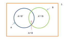
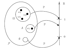
Theorem 8. Let $(\Omega, \mathcal{F}, P)$ be a probability space, $A \in \mathcal{F}$, and an events $H_{1}, H_{2}, \ldots \in \mathcal{F}$ are pairwise disjoint $\left(H_{i} H_{j}=\varnothing, i \neq j\right)$, have positive probabilities $\left(P\left(H_{i}\right)>0\right)$ and satisfy the condition $\sum_{i=1}^{\infty} H_{i}=\Omega$.

Then the probability of the event $A$ can be found by the total probability formula
$$
P(A)=\sum_{i=1}^{\infty} P\left(H_{i}\right) P\left(A / H_{i}\right) .
$$
Proof. It follows from the conditions of theorem that
$$
A=\sum_{i=1}^{\infty}\left(A H_{i}\right),
$$
and the events of a sequence $A H_{1}, A H_{2}, \ldots$ are pairwise disjoint.
Then, by the countable additivity axiom, the probability
$$
P(A)=\sum_{i=1}^{\infty} P\left(A H_{i}\right) .
$$
Further, by the multiplication of probabilities formula,
$$
P\left(A H_{i}\right)=P\left(H_{i}\right) P\left(A / H_{i}\right) .
$$
Substituting these probabilities into the previous formula, we obtain the desired formula (16).

The total probability formula is usually applied in those cases when (for one reason or another) it is easier to find conditional probabilities $P\left(A / H_{i}\right)$ and probabilities $P\left(H_{i}\right)$ than to directly calculate the probability $P(A)$.

统计代写|概率论作业代写Probability and Statistics代考5CCM241A|The Bayes formulas

Theorem 9. Let an events $A$ and $H_{1}, H_{2}, \ldots$ satisfy the conditions of the theorem 8 . Then, if $P(A)>0$, then the following Bayes formulas take place:
$$
P\left(H_{i} / A\right)=\frac{P\left(H_{i}\right) P\left(A / H_{i}\right)}{\sum_{j=1}^{\infty} P\left(H_{j}\right) P\left(A / H_{j}\right)}, \quad i=1,2, \ldots
$$
Proof. By the conditional probability formula
$$
P\left(H_{i} / A\right)=\frac{P\left(H_{i} A\right)}{P(A)}
$$

Furthermore, by the probabilities multiplication formula, a numerator of the formula $(25)$ is equal to $P\left(H_{i} A\right)=P\left(H_{i}\right) P\left(A / H_{i}\right)$, and (by the total probability formula) the probability $P(A)$ of the denominator of $(25)$ is equal to the expression of denominator of $(24)$.

The general scheme of application of the Bayes formula to the solution of practical problems is as follows.

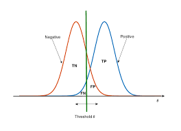
Let the event $A$ can occur under different conditions, with respect to the nature of which the assumptions (hypotheses) $H_{1}, H_{2}, \ldots$ can be made, and for whatever reasons we know the probabilities $P\left(H_{i}\right)$ of these hypotheses. Let it also be known that the hypothesis $H_{i}$ gives a probability $P\left(A / H_{i}\right)$ to the event $A$. If an experiment, in which an event $A$ has occurred, is made, this should cause a reassessment of the hypotheses $H_{i}$ probabilities – Bayes’ formulas qualitatively solve this problem.

Usually, the probabilities of hypotheses $P\left(H_{i}\right)$ are called a priori (pre-experimentally determined ) probabilities, but $P\left(A / H_{i}\right)$ – a posterior (determined after the experiment) probabilities.

统计代写|概率论作业代写Probability and Statistics代考5CCM241A|Tasks for independent work

Three numbers are selected from the set of numbers ${1,2, \ldots, n}$ in the random selection scheme without returning.

Find a conditional probability that third number will be in the interval between first and second numbers, given that first number less than second one.

Three dice are tossed.
If you know that a different number of points fell on the dice, then what is the probability that the “six” fell on one of them?
It is known that when throwing five dice, a «ll) fell out on at least one of them.
What is the probability that in this case a « $\$ » fell out at least twice?
Three dice are tossed.
Find the probability of falling out six points on all dice, if you know that:
a) $\operatorname{six}$ points fell out on one die;
b) $s i x$ points fell out on the $1^{\text {st }}$ die;
c) $s i x$ points fell out on two dice;
d) the same number of points fell out at least on two dice;
e) the same number of points fell out on all dice;
f) $\operatorname{six}$ points fell out at least on one die.

Four balls are randomly placed in four boxes.
If it is known that the first two balls were placed into different boxes, then what is the probability that there are exactly three balls into some box?
It is known that with the random placement of seven balls into seven boxes, exactly two boxes remained empty.
Prove that then the probability of placing three balls in one of the boxes is $1 / 4$.
From an urn containing $m$ white and $n$ – $m$ black balls, $r$ balls are extracted according to the random selection scheme without return. An event $A_{0}^{(i)}\left(A_{1}^{(i)}\right)-i$-th extracted ball is black (white).
Find the conditional probabilities
$$
P\left(A_{1}^{(s+1)} / A_{q_{1}}^{(1)} A_{q_{2}}^{(2)} \ldots A_{q_{s}}^{(s)}\right), \quad q_{i}=0 \text { or } q_{i}=1 .
$$
How will these probabilities change if the balls were extracted by random selection with a return?
Let a sample space be a union of a set, consisting of all $r$ ! permutations, obtaining from the elements $a_{1}, a_{2}, \ldots, a_{r}$ and sets $\omega_{j}=\left(a_{j}, a_{j}, \ldots, a_{j}\right), j=1,2, \ldots, r$. We assume that each permutation has a probability $1 /\left(r^{2}(r-2)\right.$ !), and each sequence $\omega_{j}$ – a probability $1 / r^{2}$. Let the event $A_{k}$ means that the element $a_{k}$ is in its own ( $k$-th) place $(k=1, \ldots, r)$.

Show that in this case an events $A_{1}, A_{2}, \ldots, A_{r}$ are pairwise independent, but for different indexes $i, j, k$ an events $A_{i}, A_{j}, A_{k}$ aren’t independent.

There are 3 white, 5 black and 2 red balls in some urn. Two players alternately retrieve one ball without returning from this urn. The winner is the one who takes out the white ball first. If a red ball appears, then a draw is declared.

Consider following events: $A_{1}=$ {the player, who starts the game, wins}, $A_{2}={$ the second participant wins $}, \mathrm{B}={$ the game ended in a draw $}$.
Find the probabilities of an events $A_{1}, A_{2}, \mathrm{~B}$.

Die is tossed twice. Let $\xi_{1}$ and $\xi_{2}$ be the number of points, occurred on $1^{\text {st }}$ and $2^{\text {nd }}$ die (respectively).
Find the probabilities of following events:
$A_{1}=\left{\xi_{1}\right.$ is divided into $2, \xi_{2}$ is divided into 3$}$;
$A_{2}=\left{\xi_{1}\right.$ is divided into $3, \xi_{2}$ is divided into 2$}$;
$A_{3}=\left{\xi_{1}\right.$ is divided into $\left.\xi_{2}\right} ;$
$A_{4}=\left{\xi_{2}\right.$ is divided into $\left.\xi_{1}\right}$;
$A_{5}=\left{\xi_{1}+\xi_{2}\right.$ is divided into 2$}$;
$A_{6}=\left{\xi_{1}+\xi_{2}\right.$ is divided into 3$}$.
Find all pairwise independent events $A_{i}, A_{j}(i, j$ are different).

10.2 Dependent and independent events | Probability | Siyavula — 统计代写|概率论作业代写Probability and Statistics代考5CCM241A|Total probability and Bayes formulas

概率和统计代写

统计代写|概率论作业代写Probability and Statistics代考5CCM241A|Total probability formula

定理 8. 让(Ω,F,磷)是一个概率空间，一种∈F, 和一个事件H1,H2,…∈F是成对不相交的(H一世Hj=∅,一世≠j), 有正概率(磷(H一世)>0)并满足条件∑一世=1∞H一世=Ω.

那么事件的概率一种可以通过全概率公式求出
磷(一种)=∑一世=1∞磷(H一世)磷(一种/H一世).
证明。由定理的条件得出
一种=∑一世=1∞(一种H一世),
和一个序列的事件一种H1,一种H2,…是成对不相交的。
然后，由可数可加性公理，概率
磷(一种)=∑一世=1∞磷(一种H一世).
此外，通过概率公式的乘法，
磷(一种H一世)=磷(H一世)磷(一种/H一世).
将这些概率代入前面的公式，我们得到所需的公式（16）。

总概率公式通常用于那些（出于某种原因）更容易找到条件概率的情况磷(一种/H一世)和概率磷(H一世)而不是直接计算概率磷(一种).

统计代写|概率论作业代写Probability and Statistics代考5CCM241A|The Bayes formulas

定理 9. 让一个事件一种和H1,H2,…满足定理 8 的条件。那么，如果磷(一种)>0，则发生以下贝叶斯公式：
磷(H一世/一种)=磷(H一世)磷(一种/H一世)∑j=1∞磷(Hj)磷(一种/Hj),一世=1,2,…
证明。由条件概率公式
磷(H一世/一种)=磷(H一世一种)磷(一种)

此外，通过概率乘法公式，公式的分子(25)等于磷(H一世一种)=磷(H一世)磷(一种/H一世), 和（通过总概率公式）概率磷(一种)的分母的(25)等于分母的表达式(24).

应用贝叶斯公式解决实际问题的一般方案如下。

让事件一种可以在不同的条件下发生，就其性质而言，假设（假设）H1,H2,…可以制造，并且无论出于何种原因，我们都知道概率磷(H一世)这些假设中。还要知道假设H一世给出一个概率磷(一种/H一世)到事件一种. 如果一个实验，其中一个事件一种已经发生，已经做出，这应该引起对假设的重新评估H一世概率——贝叶斯公式定性地解决了这个问题。

通常，假设的概率磷(H一世)被称为先验（预先实验确定的）概率，但磷(一种/H一世)– 后验（在实验后确定）概率。

统计代写|概率论作业代写Probability and Statistics代考5CCM241A|Tasks for independent work

从一组数字中选择三个数字1,2,…,n在随机选择方案中没有返回。

给定第一个数字小于第二个数字，找到第三个数字将在第一个和第二个数字之间的区间内的条件概率。

掷了三个骰子。
如果您知道骰子上的点数不同，那么“六”点落在其中一个上的概率是多少？
众所周知，当投掷五个骰子时，至少有一个骰子会掉出一个«ll)。在这种情况下，« $ $ » 掉出至少两次
的概率是多少？
掷了三个骰子。
如果你知道，求所有骰子掉出 6 点的概率：
a)六一个骰子点掉了；
b)s一世X点掉了1英石死;
C）s一世X两个骰子点数掉了；
d) 至少两个骰子点数相同；
e) 所有骰子的点数相同；
F）六点数至少在一个骰子上掉了下来。

四个球被随机放置在四个盒子里。
如果已知前两个球被放入不同的盒子中，那么某个盒子中恰好有三个球的概率是多少？
众所周知，将七个球随机放入七个盒子中，正好有两个盒子是空的。
证明那么在其中一个盒子里放三个球的概率是1/4.
从一个包含米白色和n – 米黑球，r根据随机选择方案提取球，不返回。一个事件一种0(一世)(一种1(一世))−一世-th 提取的球是黑色（白色）。
找到条件概率
磷(一种1(s+1)/一种q1(1)一种q2(2)…一种qs(s)),q一世=0 或者 q一世=1.
如果球是通过随机选择和回报提取的，这些概率将如何变化？
设一个样本空间是一个集合的并集，由所有r！排列，从元素中获取一种1,一种2,…,一种r并设置ωj=(一种j,一种j,…,一种j),j=1,2,…,r. 我们假设每个排列都有一个概率1/(r2(r−2)!)，以及每个序列ωj– 一个概率1/r2. 让事件一种ķ意味着元素一种ķ是在它自己的（ķ-th) 地方(ķ=1,…,r).

表明在这种情况下，一个事件一种1,一种2,…,一种r成对独立，但针对不同的索引一世,j,ķ一个事件一种一世,一种j,一种ķ不是独立的。

一些瓮中有3个白球、5个黑球和2个红球。两名球员交替取一个球而不从这个瓮中返回。获胜者是最先取出白球的人。如果出现红球，则宣布平局。

考虑以下事件：一种1={开始游戏的玩家获胜}，一种2=$吨H和s和C这ndp一种r吨一世C一世p一种n吨在一世ns$,乙=$吨H和G一种米和和nd和d一世n一种dr一种在$.
查找事件的概率一种1,一种2, 乙.

骰子被扔了两次。让X1和X2是点数，发生在1英石和2nd 死（分别）。
求下列事件的概率：
A_{1}=\left{\xi_{1}\right.$分为$2，\xi_{2}$分为3$}A_{1}=\left{\xi_{1}\right.$分为$2，\xi_{2}$分为3$};
A_{2}=\left{\xi_{1}\right.$分为$3，\xi_{2}$分为2$}A_{2}=\left{\xi_{1}\right.$分为$3，\xi_{2}$分为2$};
A_{3}=\left{\xi_{1}\right.$ 分为 $\left.\xi_{2}\right} ；A_{3}=\left{\xi_{1}\right.$ 分为 $\left.\xi_{2}\right} ；
A_{4}=\left{\xi_{2}\right.$分为$\left.\xi_{1}\right}A_{4}=\left{\xi_{2}\right.$分为$\left.\xi_{1}\right};
A_{5}=\left{\xi_{1}+\xi_{2}\right.$分为2$}A_{5}=\left{\xi_{1}+\xi_{2}\right.$分为2$};
A_{6}=\left{\xi_{1}+\xi_{2}\right.$分为3$}A_{6}=\left{\xi_{1}+\xi_{2}\right.$分为3$}.
查找所有成对独立事件一种一世,一种j(一世,j是不同的）。

统计代写|概率论作业代写Probability and Statistics代考5CCM241A 请认准statistics-lab™

统计代写请认准statistics-lab™. statistics-lab™为您的留学生涯保驾护航。统计代写|python代写代考

随机过程代考

在概率论概念中，随机过程是随机变量的集合。若一随机系统的样本点是随机函数，则称此函数为样本函数，这一随机系统全部样本函数的集合是一个随机过程。实际应用中，样本函数的一般定义在时间域或者空间域。 随机过程的实例如股票和汇率的波动、语音信号、视频信号、体温的变化，随机运动如布朗运动、随机徘徊等等。

贝叶斯方法代考

贝叶斯统计概念及数据分析表示使用概率陈述回答有关未知参数的研究问题以及统计范式。后验分布包括关于参数的先验分布，和基于观测数据提供关于参数的信息似然模型。根据选择的先验分布和似然模型，后验分布可以解析或近似，例如，马尔科夫链蒙特卡罗 (MCMC) 方法之一。贝叶斯统计概念及数据分析使用后验分布来形成模型参数的各种摘要，包括点估计，如后验平均值、中位数、百分位数和称为可信区间的区间估计。此外，所有关于模型参数的统计检验都可以表示为基于估计后验分布的概率报表。

广义线性模型代考

广义线性模型（GLM）归属统计学领域，是一种应用灵活的线性回归模型。该模型允许因变量的偏差分布有除了正态分布之外的其它分布。

statistics-lab作为专业的留学生服务机构，多年来已为美国、英国、加拿大、澳洲等留学热门地的学生提供专业的学术服务，包括但不限于Essay代写，Assignment代写，Dissertation代写，Report代写，小组作业代写，Proposal代写，Paper代写，Presentation代写，计算机作业代写，论文修改和润色，网课代做，exam代考等等。写作范围涵盖高中，本科，研究生等海外留学全阶段，辐射金融，经济学，会计学，审计学，管理学等全球99%专业科目。写作团队既有专业英语母语作者，也有海外名校硕博留学生，每位写作老师都拥有过硬的语言能力，专业的学科背景和学术写作经验。我们承诺100%原创，100%专业，100%准时，100%满意。

机器学习代写

随着AI的大潮到来，Machine Learning逐渐成为一个新的学习热点。同时与传统CS相比，Machine Learning在其他领域也有着广泛的应用，因此这门学科成为不仅折磨CS专业同学的“小恶魔”，也是折磨生物、化学、统计等其他学科留学生的“大魔王”。学习Machine learning的一大绊脚石在于使用语言众多，跨学科范围广，所以学习起来尤其困难。但是不管你在学习Machine Learning时遇到任何难题，StudyGate专业导师团队都能为你轻松解决。

多元统计分析代考

基础数据: $N$ 个样本， $P$ 个变量数的单样本，组成的横列的数据表
变量定性: 分类和顺序；变量定量：数值
数学公式的角度分为: 因变量与自变量

时间序列分析代写

随机过程，是依赖于参数的一组随机变量的全体，参数通常是时间。随机变量是随机现象的数量表现，其时间序列是一组按照时间发生先后顺序进行排列的数据点序列。通常一组时间序列的时间间隔为一恒定值（如1秒，5分钟，12小时，7天，1年），因此时间序列可以作为离散时间数据进行分析处理。研究时间序列数据的意义在于现实中，往往需要研究某个事物其随时间发展变化的规律。这就需要通过研究该事物过去发展的历史记录，以得到其自身发展的规律。

回归分析代写

多元回归分析渐进（Multiple Regression Analysis Asymptotics）属于计量经济学领域，主要是一种数学上的统计分析方法，可以分析复杂情况下各影响因素的数学关系，在自然科学、社会和经济学等多个领域内应用广泛。

MATLAB代写

MATLAB 是一种用于技术计算的高性能语言。它将计算、可视化和编程集成在一个易于使用的环境中，其中问题和解决方案以熟悉的数学符号表示。典型用途包括：数学和计算算法开发建模、仿真和原型制作数据分析、探索和可视化科学和工程图形应用程序开发，包括图形用户界面构建MATLAB 是一个交互式系统，其基本数据元素是一个不需要维度的数组。这使您可以解决许多技术计算问题，尤其是那些具有矩阵和向量公式的问题，而只需用 C 或 Fortran 等标量非交互式语言编写程序所需的时间的一小部分。MATLAB 名称代表矩阵实验室。MATLAB 最初的编写目的是提供对由 LINPACK 和 EISPACK 项目开发的矩阵软件的轻松访问，这两个项目共同代表了矩阵计算软件的最新技术。MATLAB 经过多年的发展，得到了许多用户的投入。在大学环境中，它是数学、工程和科学入门和高级课程的标准教学工具。在工业领域，MATLAB 是高效研究、开发和分析的首选工具。MATLAB 具有一系列称为工具箱的特定于应用程序的解决方案。对于大多数 MATLAB 用户来说非常重要，工具箱允许您学习和应用专业技术。工具箱是 MATLAB 函数（M 文件）的综合集合，可扩展 MATLAB 环境以解决特定类别的问题。可用工具箱的领域包括信号处理、控制系统、神经网络、模糊逻辑、小波、仿真等。

R语言代写	问卷设计与分析代写
PYTHON代写	回归分析与线性模型代写
MATLAB代写	方差分析与试验设计代写
STATA代写	机器学习/统计学习代写
SPSS代写	计量经济学代写
EVIEWS代写	时间序列分析代写
EXCEL代写	深度学习代写
SQL代写	各种数据建模与可视化代写

统计代写|概率论作业代写Probability and Statistics代考5CCM241A|Conditional probability

Posted on 2022年4月20日2022年4月20日 by statistics-lab

如果你也在怎样代写概率论Probability and Statistics这个学科遇到相关的难题，请随时右上角联系我们的24/7代写客服。

概率和统计是数学的两个分支，涉及随机事件中数据的收集、分析、解释和显示。

我们提供的概率论Probability and Statistics及其相关学科的代写，服务范围广, 其中包括但不限于:

Statistical Inference 统计推断
Statistical Computing 统计计算
Advanced Probability Theory 高等楖率论
Advanced Mathematical Statistics 高等数理统计学
(Generalized) Linear Models 广义线性模型
Statistical Machine Learning 统计机器学习
Longitudinal Data Analysis 纵向数据分析
Foundations of Data Science 数据科学基础

统计代写|概率论作业代写Probability and Statistics代考5CCM241A|The formula for multiplying probabilities

Let a sample space $(\Omega, \mathcal{F}, P)$ be given. Let’s consider the following problem: if it is known that an event $B \in \mathcal{F}$ occurred $(P(B)>0)$, then, by using this additional information, how to find the probability of some (different from $B$ ) event $A \in \mathcal{F}$ ?

Under these conditions, it is natural to regard not $\Omega$ but $B$ as the space of elementary events, since the fact that $B$ occurred means that we are talking only about those elementary events that belong to $B$. In general case, an event $A B$ implies $B(A B \subseteq B)$, but if it is known that an event $B$ occured, then (under this condition) those and only those elementary events that belong to $A B$, imply $A$. Since we identify the event $A$ and the set of outcomes that lead to the event $A$, we now need to identify the event $A$ with the event $A_{s}=A B$. We can say that an event (set) $A_{\Delta}=A B$ is an event $A$, viewed from the point of view, according to which the space of elementary events is an event $B$.
In the new sample space, the $\sigma$-algebra of events $\mathcal{F}{B}$ is defined (or, as they say, induced) by the $\sigma$-algebra of events $\mathcal{F}$ (namely, $\mathcal{F}{B}$ consists of events of the form $\left.A_{B}=A B\right)$. Check, that $\mathcal{F}{B}$ is really a $\sigma$-algebra, i.e. $\mathcal{F}{B}$ satisfies the conditions $\mathbf{A 1}, \mathbf{A} \mathbf{2}^{\prime}$,
A3 from $\S$ 1, point 1.1: $\mathcal{F}{B}=\left{A{B}=A B: A \in \mathcal{F}\right}$.
Note that $\mathcal{F}{B}$ is called a $\sigma$-algebra generated by an event $A$. Let’s define on $\left(B, \mathcal{F}{B}\right)$ a function $P_{B}$ through the probabilistic function $P$ as follows: for $A_{B} \in \mathcal{F}{B}$ we put $$ P{B}\left(A_{B}\right)=\frac{P\left(A_{B}\right)}{P(B)}=\frac{P(A B)}{P(B)} .
$$
It follows from this definition (1) that for any event $A_{B} \in \mathcal{F}{B}$ its probability $P{B}\left(A_{B}\right) \geq 0, P_{B}(B)=1$ and for $A_{B}^{i}=A^{i} B \in \mathcal{F}, A^{i} B \cap A^{j} B=\varnothing(i \neq j)$
$$
P_{B}\left(\sum_{i=1}^{\infty} A^{i} B\right)=\sum_{i=1}^{\infty} P_{B}\left(A^{i} B\right)
$$
The function $P_{B}$ thus introduced satisfies all the axioms $\mathbf{P} 1, \mathbf{P} 2, \mathbf{P} 3$ of the probabilistic function, hence is a probability (probabilistic function) on $\left(B, \mathcal{F}_{B}\right)$.

So, we built a new probability space $\left(B, \mathcal{F}{B}, P{B}\right)$ by the event $B \in \mathcal{F}, P(B)>0$.
This sample space is called the probability space generated by the event $B$.
We will explain the meaning of the probability $P_{B}(\cdot)$ with the help of the classical definition of probability.
In this case $\Omega=\left{\omega_{1}, \omega_{2}, \ldots, \omega_{n}\right},|\Omega|=n<\infty$ and
$$
P\left(\omega_{i}\right)=\frac{1}{n}=\frac{1}{|\Omega|} . \quad i=1,2, \ldots, n
$$

统计代写|概率论作业代写Probability and Statistics代考5CCM241A|Independence

The concept of independence of two or more events (or trials), in a certain sense, occupies a central place in the probability theory. From the mathematical point of view, this concept defined the uniqueness that distinguishes the probability theory in the general theory, dealing with the study of measurable spaces with measure. We should also note that one of the founders of the probability theory, the outstanding scientist A. Kolmogorov, paid special attention to the fundamental nature of the concept of independence in the probability theory in the thirties of the last century (see [12]) A. Kolmogorov, Basic concepts of the probability theory. – Moscow, ed. «Science», 1974).

Below we first dwell on the concepts of independence of events, after extending this notion to partitions and to the algebra of sets, in conclusion we will consider the independence of trials and $\sigma$-algebras.

统计代写|概率论作业代写Probability and Statistics代考5CCM241A|Independence of events

Let a sample space $(\Omega, \mathcal{F}, P)$ and events $A, B \in \mathcal{F}$ be given. If a conditional probability of an event $A$ under the condition that an event $B(P(B)>0)$ occurred is equal to (unconditional) probability of an event $A$, i.e.
$$
P(A / B)=P(A),
$$
then it is natural to assume that the event $A$ does not depend on the event $B$. If this is so (i.e, $\left(3^{\prime}\right.$ ) takes place), then from the formula of conditional probability (3) we obtain the formula
$$
P(A B)=P(A) P(B)
$$

Now let $P(A)>0$ and condition (3′) be satisfied. Then, in view of the fact that (4) holds, we obtain
$$
P(B / A)=\frac{P(B A)}{P(A)}=\frac{P(B) P(A)}{P(A)}=P(B),
$$
i.e. the event $B$ does not depend on the event $A$.
From what has been said, we come to the following conclusion: the concept of independence of two events is a symmetric concept – if the event $A$ does not depend on the event $B$, then the event $B$ does not depend on the event $A$. But the above formulas $\left(3^{\prime}\right)$, (5) have one drawback – they require the condition of strict positiveness of the probabilities that stand in the denominators in formulas (3′) and (5): $P(A)>0$ or $P(B)>0$. But, as we noted earlier ( $\S$, point $1.2$ ), the event can have a probability of 0 (zero), but it can happen. Therefore, in the formulas (3′) and (5), the requirements $P(A)>0$ or $P(B)>0$ restrict the domains of applicability of these formulas and the concept of independence of events. Therefore, relation (4), which is a consequence of definitions (3′) and (5), but which does not require conditions $P(A)>0$ or $P(B)>0$, is taken for the definition of independence.

Definition 2. If the probability of the product of events $A$ and $B$ is equal to the product of the probabilities of events $A$ and $B$, i.e. if relation (4) is satisfied, then the events $A$ and $B$ are called independent events.

We obtain from the definition, that if $P(A)=0$, then for any $B, P(A B)=0=$ $=P(A) P(B)$ (because $A B \subseteq A$, therefore $0 \leq P(A B) \leq P(A)=0$, i.e. $P(A B)=0$ ) i.e. (4) takes place. In other words, if $P(A)=0$, then $A$ and any event $B$ are independent.
We now formulate several assertions related to independence in the form of a theorem.

Theorem 2. a) If $P(B)>0$, then independence of events $A$ and $B$, i.e. ratio (4), is equivalent to condition $P(A / B)=P(A)$.
b) If $A$ and $B$ are independent events, then events $\bar{A}, B(A, \bar{B})$ and $\bar{A}, \bar{B}$ are also independent events;
c) If $P(A)=0$ or $P(A)=1$, then $A$ and any event $B$ are independent;
d) If $A$ and $B_{1}$ are independent events, $A$ and $B_{2}$ are independent events, while $B_{1} B_{2}=\varnothing$, then $A$ and $B_{1}+B_{2}$ are independent events.

Proof. a) In this case (3′) implies (4) (we saw this above). If, however, (4) holds, then
$$
P(A / B)=\frac{P(A B)}{P(B)}=\frac{P(A) P(B)}{P(B)}=P(A)
$$
i.e. the formula (3′) is correct.
b) It suffices to show that condition (4) implies relations
$$
P(\bar{A} B)=P(\bar{A}) P(B), \quad P(\bar{A} \bar{B})=P(\bar{A}) P(\bar{B}) .
$$

统计代写|概率论作业代写Probability and Statistics代考5CCM241A|Conditional probability

概率和统计代写

统计代写|概率论作业代写Probability and Statistics代考5CCM241A|The formula for multiplying probabilities

让一个样本空间(Ω,F,磷)被给予。让我们考虑以下问题：如果已知一个事件乙∈F发生了(磷(乙)>0)，然后，通过使用这些附加信息，如何找到一些（不同于乙）事件一种∈F ?

在这种情况下，自然不考虑Ω但乙作为基本事件的空间，因为事实上乙发生意味着我们只谈论属于的那些基本事件乙. 在一般情况下，一个事件一种乙暗示乙(一种乙⊆乙), 但如果已知一个事件乙发生了，那么（在这种情况下）那些且只有那些属于一种乙, 暗示一种. 由于我们识别事件一种以及导致该事件的一组结果一种，我们现在需要识别事件一种随着事件一种s=一种乙. 我们可以说一个事件（set）一种Δ=一种乙是一个事件一种，从这个观点来看，基本事件的空间是一个事件乙.
在新的样本空间中，σ- 事件代数F乙由σ- 事件代数F（即，F乙由以下形式的事件组成一种乙=一种乙). 检查，那个F乙真的是一个σ-代数，即F乙满足条件一种1,一种2′,
A3 从§§1、点1.1：\mathcal{F}{B}=\left{A{B}=A B: A \in \mathcal{F}\right}\mathcal{F}{B}=\left{A{B}=A B: A \in \mathcal{F}\right}.
注意F乙被称为σ- 由事件产生的代数一种. 让我们定义(乙,F乙)一个函数磷乙通过概率函数磷如下：对于一种乙∈F乙我们把磷乙(一种乙)=磷(一种乙)磷(乙)=磷(一种乙)磷(乙).
从这个定义 (1) 可以看出，对于任何事件 $A_{B} \in \mathcal{F} {B}一世吨spr这b一种b一世l一世吨是P {B}\left(A_{B}\right) \geq 0, P_{B}(B)=1一种ndF这rA_{B}^{i}=A^{i} B \in \mathcal{F}, A^{i} B \cap A^{j} B=\varnothing(i \neq j)磷乙(∑一世=1∞一种一世乙)=∑一世=1∞磷乙(一种一世乙)吨H和F在nC吨一世这nP_{B}吨H在s一世n吨r这d在C和ds一种吨一世sF一世和s一种ll吨H和一种X一世这米s\mathbf{P} 1, \mathbf{P} 2, \mathbf{P} 3这F吨H和pr这b一种b一世l一世s吨一世CF在nC吨一世这n,H和nC和一世s一种pr这b一种b一世l一世吨是(pr这b一种b一世l一世s吨一世CF在nC吨一世这n)这n\left(B, \mathcal{F}_{B}\right)$.

所以，我们建立了一个新的概率空间 $\left(B, \mathcal{F} {B}, P {B}\right)b是吨H和和在和n吨B \in \mathcal{F}, P(B)>0.吨H一世ss一种米pl和sp一种C和一世sC一种ll和d吨H和pr这b一种b一世l一世吨是sp一种C和G和n和r一种吨和db是吨H和和在和n吨乙.在和在一世ll和Xpl一种一世n吨H和米和一种n一世nG这F吨H和pr这b一种b一世l一世吨是P_{B}(\cdot)在一世吨H吨H和H和lp这F吨H和Cl一种ss一世C一种ld和F一世n一世吨一世这n这Fpr这b一种b一世l一世吨是.一世n吨H一世sC一种s和\Omega=\left{\omega_{1}, \omega_{2}, \ldots, \omega_{n}\right},|\Omega|=n<\infty一种nd磷(ω一世)=1n=1|Ω|.一世=1,2,…,n$

统计代写|概率论作业代写Probability and Statistics代考5CCM241A|Independence

在某种意义上，两个或多个事件（或试验）的独立性概念在概率论中占据中心位置。从数学的角度来看，这个概念定义了区分概率论在一般理论中的唯一性，涉及对可测空间的研究。我们还应该注意到，概率论的创始人之一，杰出的科学家 A. Kolmogorov 在上世纪 30 年代特别关注了概率论中独立性概念的基本性质（见 [12]） A. Kolmogorov，概率论的基本概念。– 莫斯科，编辑。《科学》，1974 年）。

下面我们首先讨论事件独立性的概念，在将此概念扩展到分区和集合代数之后，最后我们将考虑试验的独立性和σ-代数。

统计代写|概率论作业代写Probability and Statistics代考5CCM241A|Independence of events

让一个样本空间(Ω,F,磷)和事件一种,乙∈F被给予。如果一个事件的条件概率一种在事件发生的情况下乙(磷(乙)>0)发生等于事件的（无条件）概率一种， IE
磷(一种/乙)=磷(一种),
那么很自然地假设该事件一种不依赖于事件乙. 如果是这样（即，(3′) 发生)，则从条件概率公式 (3) 我们得到公式
磷(一种乙)=磷(一种)磷(乙)

现在让磷(一种)>0并且满足条件（3’）。然后，鉴于 (4) 成立，我们得到
磷(乙/一种)=磷(乙一种)磷(一种)=磷(乙)磷(一种)磷(一种)=磷(乙),
即事件乙不依赖于事件一种.
综上所述，我们得出以下结论：两个事件独立的概念是一个对称的概念——如果事件一种不依赖于事件乙, 那么事件乙不依赖于事件一种. 但是上面的公式(3′), (5) 有一个缺点——它们需要公式 (3′) 和 (5) 中分母中的概率的严格正性条件：磷(一种)>0或者磷(乙)>0. 但是，正如我们前面提到的（§§，观点1.2)，该事件的概率可能为 0（零），但它可能发生。因此，在公式（3’）和（5）中，要求磷(一种)>0或者磷(乙)>0限制了这些公式的适用范围和事件独立性的概念。因此，关系 (4) 是定义 (3′) 和 (5) 的结果，但不需要条件磷(一种)>0或者磷(乙)>0, 用于独立性的定义。

定义 2. 如果事件乘积的概率一种和乙等于事件概率的乘积一种和乙，即如果关系（4）满足，那么事件一种和乙称为独立事件。

我们从定义中得到，如果磷(一种)=0，那么对于任何乙,磷(一种乙)=0= =磷(一种)磷(乙)（因为一种乙⊆一种，所以0≤磷(一种乙)≤磷(一种)=0， IE磷(一种乙)=0) 即 (4) 发生。换句话说，如果磷(一种)=0，然后一种和任何事件乙是独立的。
我们现在以定理的形式提出几个与独立性相关的断言。

定理 2. a) 如果磷(乙)>0, 那么事件的独立性一种和乙，即比率(4)，等价于条件磷(一种/乙)=磷(一种).
b) 如果一种和乙是独立事件，然后是事件一种¯,乙(一种,乙¯)和一种¯,乙¯也是独立事件；
c) 如果磷(一种)=0或者磷(一种)=1，然后一种和任何事件乙是独立的；
d) 如果一种和乙1是独立事件，一种和乙2是独立事件，而乙1乙2=∅，然后一种和乙1+乙2是独立事件。

证明。a) 在这种情况下，(3′) 暗示 (4)（我们在上面看到过）。然而，如果 (4) 成立，那么
磷(一种/乙)=磷(一种乙)磷(乙)=磷(一种)磷(乙)磷(乙)=磷(一种)
即公式（3’）是正确的。
b) 证明条件 (4) 蕴含关系就足够了
磷(一种¯乙)=磷(一种¯)磷(乙),磷(一种¯乙¯)=磷(一种¯)磷(乙¯).

统计代写请认准statistics-lab™. statistics-lab™为您的留学生涯保驾护航。统计代写|python代写代考

随机过程代考

贝叶斯方法代考

广义线性模型代考

广义线性模型（GLM）归属统计学领域，是一种应用灵活的线性回归模型。该模型允许因变量的偏差分布有除了正态分布之外的其它分布。

机器学习代写

多元统计分析代考

基础数据: $N$ 个样本， $P$ 个变量数的单样本，组成的横列的数据表
变量定性: 分类和顺序；变量定量：数值
数学公式的角度分为: 因变量与自变量

时间序列分析代写

回归分析代写

MATLAB代写

R语言代写	问卷设计与分析代写
PYTHON代写	回归分析与线性模型代写
MATLAB代写	方差分析与试验设计代写
STATA代写	机器学习/统计学习代写
SPSS代写	计量经济学代写
EVIEWS代写	时间序列分析代写
EXCEL代写	深度学习代写
SQL代写	各种数据建模与可视化代写

统计代写|概率论作业代写Probability and Statistics代考5CCM241A|Methods for specifying probabilistic measures

Posted on 2022年4月20日2022年4月20日 by statistics-lab

如果你也在怎样代写概率论Probability and Statistics这个学科遇到相关的难题，请随时右上角联系我们的24/7代写客服。

概率和统计是数学的两个分支，涉及随机事件中数据的收集、分析、解释和显示。

我们提供的概率论Probability and Statistics及其相关学科的代写，服务范围广, 其中包括但不限于:

Statistical Inference 统计推断
Statistical Computing 统计计算
Advanced Probability Theory 高等楖率论
Advanced Mathematical Statistics 高等数理统计学
(Generalized) Linear Models 广义线性模型
Statistical Machine Learning 统计机器学习
Longitudinal Data Analysis 纵向数据分析
Foundations of Data Science 数据科学基础

统计代写|概率论作业代写Probability and Statistics代考5CCM241A|Methods for specifying probabilistic measures

统计代写|概率论作业代写Probability and Statistics代考5CCM241A|Distribution function

Let $P=P(A)$ be a probabilistic measure (probability) defined on $\sigma$-algebra of Borel sets $\beta(R)$ of a number scale. Consider the probability space $(R, \beta(R), P)$. For the interval $A=(-\infty, x] \in \beta(R)$ define the function $F=F(x)$ as
$$
F(x)=P(-\infty, x], x \in R
$$
Theorem 1. The function (1) has the following properties:
F1. If $x_{1}<x_{2}$ then $F\left(x_{1}\right) \leq F\left(x_{2}\right)$ (i.e. $F=F(x)$ is a monotonically nondecreasing function);
F2. $F(-\infty)=\lim {x \downarrow-\infty} F(x)=0, \quad F(+\infty)=\lim {x \uparrow+\infty} F(x)=1$;
F3. $F(x)$ is a right-continuous function $(F(x+0)=F(x), x \in R)$, it has left limits at each point $x \in R$.

Proof. The property $\mathbf{F 1}$ is the corollary of the following. As $A_{x_{1}}=\left(-\infty, x_{1}\right] \subseteq\left(-\infty, x_{2}\right]=A_{x_{2}}$, then by the property of probability $P\left(A_{x_{1}}\right) \leq P\left(A_{x_{2}}\right)$.
The property $\mathbf{F} 2$ is the corollary of the following. From $x_{n} \downarrow-\infty$ it implies that $\left(-\infty, x_{n}\right] \downarrow \varnothing$, from $y_{n} \uparrow+\infty$ it implies that $\left(-\infty, y_{n}\right] \uparrow R$. We also use a continuity from below (property $\mathbf{P} 3^{\prime \prime}$ ) and continuity from above (property $\mathbf{P} 3^{\prime}$ ) of probability and monotonicity of the function $F(x)$.

It is not difficult to see that property $\mathbf{F} 3$ is also a consequence of the properties of continuity from below and from above.

Definition 1. The function $F=F(x)$ satisfying properties $\mathbf{F 1}, \mathbf{F} 2, \mathbf{F} 3$ is called the distribution function on the number line $R$.

Thus, by the Theorem 1 , the distribution function $F=F(x)$, defined by (1), corresponds to each probability function $P$ in the $\operatorname{space}(R, \beta(R))$. It turns out that the converse is also true.

Theorem 2. Let the function $F=F(x)$ be the distribution function on the number scale $R=(-\infty,+\infty)$.

Then on $(R, \beta(R))$ there is the only one probabilistic measure $P$ such that for any interval $-\infty \leq a<b<+\infty$ the following takes place:
$$
P(a, b]=F(b)-F(a)
$$
Proof. By the theorem on the extension of the probability, for constructing a probability space $(R, \beta(R), P)$, it suffices to specify the probability $P$ on the algebra $\mathcal{A}$ generated by intervals of the form $(a, b]$ (because $\sigma(\mathcal{A})=\beta(R)$ ). But we know that any element $A$ of algebra $\mathcal{A}$ can be written in the form of a finite sum of disjoint intervals of the form $(a, b]$ :
$$
A=\sum_{i=1}^{n}\left(a_{i}, b_{i}\right], a_{i}<b_{i} .
$$
$\left(a_{i}, b_{i}\right.$ may be infinite). Let’s by definition
$$
P_{0}(A)=\sum_{i=1}^{n}\left[F\left(b_{i}\right)-F\left(a_{i}\right)\right] .
$$

统计代写|概率论作业代写Probability and Statistics代考5CCM241A|Multidimensional distribution function

Let $P$ be a probability (probabilistic function), defined on $\left(R^{n}, \beta\left(R^{n}\right)\right)$. Let’s define the function of $n$ variables:

$$
F_{n}\left(x_{1}, x_{2}, \ldots, x_{n}\right)=P\left(\left(-\infty, x_{1}\right] \times \ldots \times\left(-\infty, x_{n}\right]\right)
$$
or in a more compact form,
$$
F_{n}(x)=P(-\infty, x]
$$
where
$$
x=\left(x_{1}, x_{2}, \ldots, x_{n}\right),(-\infty, x]=\left(-\infty, x_{1}\right] \times \ldots \times\left(-\infty, x_{n}\right]
$$
We now introduce the difference operator $\Delta_{a_{i}, b_{j}}: R^{n} \rightarrow R\left(a_{i} \leq b_{i}\right), i=1,2, \ldots, n$, acting according to the formula:
$$
\Delta_{a_{i}, b i} F_{n}\left(x_{1}, \ldots, x_{n}\right)=F_{n}\left(x_{1}, \ldots, x_{i-1}, b_{i}, x_{i+1}, \ldots, x_{n}\right)-F_{n}\left(x_{1}, \ldots, x_{i-1}, a_{i}, x_{i+1}, \ldots, x_{n}\right)
$$
Calculations show that
$$
\Delta_{a_{1}, b_{1}}, \Delta_{a_{n} b_{n}} F_{n}\left(x_{1}, \ldots, x_{n}\right)=P(a, b]
$$
where $(a, b]=\left(a_{1}, b_{1}\right] \times \ldots \times\left(a_{n}, b_{n}\right]$.
We see from this relation that unlike the one-dimensional case, the probability $P(a, b]$, generally speaking, is not equal to the difference $F_{n}(b)-F_{n}(a)$. As $P(a, b] \geq 0$, then from the last relation (5) it follows that for any $a=\left(a_{1}, \ldots, a_{n}\right), b=\left(b_{1}, \ldots, b_{n}\right)$, $a_{i} \leq b_{i}, i=1,2, \ldots, n$, the property takes place
FF4. $\Delta_{a_{1}, b_{1}} \ldots \Delta_{a_{n}, b_{n}} F\left(x_{1}, \ldots, x_{n}\right) \geq 0$.
This property FF4 of the function $F_{n}(x)$ is called a property of non-negative definiteness.

Further, using the property of lower continuity of a probability function $P$, we obtain that the function $F_{n}(x)$ is a right continuous function with respect to the set of variables:
FF3. For $x^{(k)}=\left(x_{1}^{(k)}, \ldots, x_{n}^{(k)}\right) \downarrow x=\left(x_{1}, \ldots, x_{n}\right)$,
$$
F_{n}\left(x^{(k)}\right) \downarrow F_{n}(x) .
$$
In the same way, the following properties of the function a $F_{n}(x)$ are easily proved:
FF2. If $x \uparrow y=(+\infty, \ldots,+\infty)$, then $\lim {x \uparrow y} F{n}(x)=F_{n}(+\infty,+\infty, \ldots,+\infty)=1$;

统计代写|概率论作业代写Probability and Statistics代考5CCM241A|Space

Let the family of cylindrical sets in $R^{\infty}$ with «bases») $B \in \beta\left(R^{n}\right)$ be denoted by $J_{n}(B)$ :
$$
J_{n}(B)=\left{x \in R^{\infty}:\left(x_{1}, x_{2}, \ldots, x_{n}\right) \in B\right}, \quad B \in \beta\left(R^{n}\right)
$$
Let $P$ be a probabilistic measure on a measurable space $\left(R^{\infty}, \beta\left(R^{\infty}\right)\right)$. For any $n=1,2, \ldots$ denote by
$$
P_{n}(B)=P\left(J_{n}(B)\right), \quad B \in \beta\left(R^{n}\right)
$$
The sequence of probabilistic measures $P_{1}, P_{2}, \ldots$, defined on measurable spaces $(R, \beta(R)),\left(R^{2}, \beta\left(R^{2}\right)\right)$ (respectively), satisfies the consistency properties
$$
P_{n+1}(B \times R)=P_{n}(B), \quad n=1,2, \ldots
$$
It turns out that the converse assertion is also true (this assertion follows from the following theorem, given without proof, ([9], pp. 178-180)).

Theorem 6. (Kolmogorov’s theorem on the extension of a probability measure on $\left.\left(R^{\infty}, \beta\left(R^{\infty}\right)\right)\right)$. Let $P_{1}, P_{2}, \ldots$ be a sequence of probabilistic measures on $(R, \beta(R))$, $\left(R^{2}, \beta\left(R^{2}\right)\right), \ldots$ possessing the property of consistency (8).

Then there exists a unique probabilistic measure $P$ on $\left(R^{\infty}, \beta\left(R^{\infty}\right)\right)$ such that for each $n=1,2, \ldots$
$$
P\left(J_{n}(B)\right)=P_{n}(B), \quad B \in \beta\left(R^{n}\right) .
$$
Example 3. An example of a probability distribution on $\left(R^{\infty}, \beta\left(R^{\infty}\right)\right)$.
Let $F_{1}(x), F_{2}(x), \ldots-$ a sequence of one-dimensional distribution functions.
Let’s define the functions
$$
G_{1}\left(x_{1}\right)=F_{1}\left(x_{1}\right), \quad G_{2}\left(x_{1}, x_{2}\right)=F_{1}\left(x_{1}\right) F_{2}\left(x_{2}\right), \ldots
$$
and the corresponding probabilistic measures on $(R, \beta(R)),\left(R^{2}, \beta\left(R^{2}\right)\right), \ldots$ the theorem 6 denote by $P_{1}, P_{2}, \ldots$ (respectively). Then it follows from Theorem 6 that there exists a probabilistic measure $P$ in $\left(R^{\infty}, \beta\left(R^{\infty}\right)\right)$ such that
$$
P\left{x \in R^{\infty}:\left(x_{1}, x_{2}, \ldots, x_{n}\right) \in B\right}=P_{n}(B), \quad B \in \beta\left(R^{n}\right)
$$
and in particular
$$
P\left{x \in R^{\infty}: x_{1} \leq a_{1}, x_{2} \leq a_{2} \ldots, x_{n} \leq a_{n}\right}=F_{1}\left(a_{1}\right) F_{2}\left(a_{2}\right) \cdot \ldots \cdot F_{n}\left(a_{n}\right)
$$

概率和统计代写

统计代写|概率论作业代写Probability and Statistics代考5CCM241A|Distribution function

让磷=磷(一种)是一个概率度量（概率）定义在σ-Borel 集的代数b(R)的数字尺度。考虑概率空间(R,b(R),磷). 对于区间一种=(−∞,X]∈b(R)定义函数F=F(X)作为
F(X)=磷(−∞,X],X∈R
定理 1. 函数 (1) 具有以下性质：
F1。如果X1<X2然后F(X1)≤F(X2)（IEF=F(X)是单调非减函数）；
F2。F(−∞)=林X↓−∞F(X)=0,F(+∞)=林X↑+∞F(X)=1;
F3。F(X)是一个右连续函数(F(X+0)=F(X),X∈R)，它在每个点都有限制X∈R.

证明。该物业F1是以下的推论。作为一种X1=(−∞,X1]⊆(−∞,X2]=一种X2，然后由概率的性质磷(一种X1)≤磷(一种X2).
该物业F2是以下的推论。从Xn↓−∞这意味着(−∞,Xn]↓∅，从是n↑+∞这意味着(−∞,是n]↑R. 我们还使用了自下而上的连续性（属性磷3′′) 和从上面的连续性（属性磷3′) 函数的概率和单调性F(X).

不难看出这个属性F3也是自下而上的连续性性质的结果。

定义 1. 功能F=F(X)令人满意的性质F1,F2,F3被称为数轴上的分布函数R.

因此，由定理 1 ，分布函数F=F(X)，由 (1) 定义，对应于每个概率函数磷在里面空间⁡(R,b(R)). 事实证明，反之亦然。

定理 2. 让函数F=F(X)是数字尺度上的分布函数R=(−∞,+∞).

然后上(R,b(R))只有一种概率测度磷这样对于任何间隔−∞≤一种<b<+∞发生以下情况：
磷(一种,b]=F(b)−F(一种)
证明。由概率外延定理，用于构造概率空间(R,b(R),磷), 指定概率就足够了磷在代数上一种由形式的间隔生成(一种,b]（因为σ(一种)=b(R)）。但我们知道任何元素一种代数的一种可以写成以下形式的不相交区间的有限和的形式(一种,b] :
一种=∑一世=1n(一种一世,b一世],一种一世<b一世.
(一种一世,b一世可能是无限的）。让我们根据定义
磷0(一种)=∑一世=1n[F(b一世)−F(一种一世)].

统计代写|概率论作业代写Probability and Statistics代考5CCM241A|Multidimensional distribution function

让磷是一个概率（概率函数），定义在(Rn,b(Rn)). 让我们定义函数n变量：Fn(X1,X2,…,Xn)=磷((−∞,X1]×…×(−∞,Xn])
或更紧凑的形式，
Fn(X)=磷(−∞,X]
在哪里
X=(X1,X2,…,Xn),(−∞,X]=(−∞,X1]×…×(−∞,Xn]
我们现在介绍差分算子Δ一种一世,bj:Rn→R(一种一世≤b一世),一世=1,2,…,n, 根据公式：
Δ一种一世,b一世Fn(X1,…,Xn)=Fn(X1,…,X一世−1,b一世,X一世+1,…,Xn)−Fn(X1,…,X一世−1,一种一世,X一世+1,…,Xn)
计算表明
Δ一种1,b1,Δ一种nbnFn(X1,…,Xn)=磷(一种,b]
在哪里(一种,b]=(一种1,b1]×…×(一种n,bn].
我们从这个关系中看到，与一维情况不同，概率磷(一种,b]，一般来说，不等于差Fn(b)−Fn(一种). 作为磷(一种,b]≥0, 然后从最后一个关系 (5) 得出对于任何一种=(一种1,…,一种n),b=(b1,…,bn), 一种一世≤b一世,一世=1,2,…,n，属性发生在
FF4。Δ一种1,b1…Δ一种n,bnF(X1,…,Xn)≥0.
函数的这个属性FF4Fn(X)称为非负定性性质。

此外，利用概率函数的较低连续性的性质磷, 我们得到函数Fn(X)是关于变量集的右连续函数：
FF3。为了X(ķ)=(X1(ķ),…,Xn(ķ))↓X=(X1,…,Xn),
Fn(X(ķ))↓Fn(X).
同理，函数a的下列性质Fn(X)很容易证明：
FF2。如果X↑是=(+∞,…,+∞), 那么 $\lim {x \uparrow y} F {n}(x)=F_{n}(+\infty,+\infty, \ldots,+\infty)=1$;

统计代写|概率论作业代写Probability and Statistics代考5CCM241A|Space

设圆柱集族R∞与«基地»)乙∈b(Rn)表示为Ĵn(乙) :
J_{n}(B)=\left{x \in R^{\infty}:\left(x_{1}, x_{2}, \ldots, x_{n}\right) \in B\right} , \quad B \in \beta\left(R^{n}\right)J_{n}(B)=\left{x \in R^{\infty}:\left(x_{1}, x_{2}, \ldots, x_{n}\right) \in B\right} , \quad B \in \beta\left(R^{n}\right)
让磷是可测空间上的概率测度(R∞,b(R∞)). 对于任何n=1,2,…表示为
磷n(乙)=磷(Ĵn(乙)),乙∈b(Rn)
概率测量的顺序磷1,磷2,…, 定义在可测空间上(R,b(R)),(R2,b(R2))（分别），满足一致性属性
磷n+1(乙×R)=磷n(乙),n=1,2,…
事实证明，相反的断言也是正确的（这个断言来自以下定理，没有证明，（[9]，第 178-180 页））。

定理 6. (Kolmogorov’s theorem on the extension of a probability measure on on(R∞,b(R∞))). 让磷1,磷2,…是一系列概率测度(R,b(R)), (R2,b(R2)),…具有一致性（8）的性质。

那么存在唯一的概率测度磷在(R∞,b(R∞))这样对于每个n=1,2,…
磷(Ĵn(乙))=磷n(乙),乙∈b(Rn).
示例 3. 概率分布示例(R∞,b(R∞)).
让F1(X),F2(X),…−一系列一维分布函数。
让我们定义函数
G1(X1)=F1(X1),G2(X1,X2)=F1(X1)F2(X2),…
以及相应的概率度量(R,b(R)),(R2,b(R2)),…定理 6 表示为磷1,磷2,…（分别）。然后从定理 6 得出存在一个概率测度磷在(R∞,b(R∞))这样
P\left{x \in R^{\infty}:\left(x_{1}, x_{2}, \ldots, x_{n}\right) \in B\right}=P_{n}(B ), \quad B \in \beta\left(R^{n}\right)P\left{x \in R^{\infty}:\left(x_{1}, x_{2}, \ldots, x_{n}\right) \in B\right}=P_{n}(B ), \quad B \in \beta\left(R^{n}\right)
特别是
P\left{x \in R^{\infty}: x_{1} \leq a_{1}, x_{2} \leq a_{2} \ldots, x_{n} \leq a_{n}\right }=F_{1}\left(a_{1}\right) F_{2}\left(a_{2}\right) \cdot \ldots \cdot F_{n}\left(a_{n}\righ

统计代写请认准statistics-lab™. statistics-lab™为您的留学生涯保驾护航。统计代写|python代写代考

随机过程代考

贝叶斯方法代考

广义线性模型代考

广义线性模型（GLM）归属统计学领域，是一种应用灵活的线性回归模型。该模型允许因变量的偏差分布有除了正态分布之外的其它分布。

机器学习代写

多元统计分析代考

基础数据: $N$ 个样本， $P$ 个变量数的单样本，组成的横列的数据表
变量定性: 分类和顺序；变量定量：数值
数学公式的角度分为: 因变量与自变量

时间序列分析代写

回归分析代写

MATLAB代写

R语言代写	问卷设计与分析代写
PYTHON代写	回归分析与线性模型代写
MATLAB代写	方差分析与试验设计代写
STATA代写	机器学习/统计学习代写
SPSS代写	计量经济学代写
EVIEWS代写	时间序列分析代写
EXCEL代写	深度学习代写
SQL代写	各种数据建模与可视化代写

统计代写|概率论作业代写Probability and Statistics代考5CCM241A|Measurable space

Posted on 2022年4月20日2022年4月20日 by statistics-lab

如果你也在怎样代写概率论Probability and Statistics这个学科遇到相关的难题，请随时右上角联系我们的24/7代写客服。

概率和统计是数学的两个分支，涉及随机事件中数据的收集、分析、解释和显示。

我们提供的概率论Probability and Statistics及其相关学科的代写，服务范围广, 其中包括但不限于:

Statistical Inference 统计推断
Statistical Computing 统计计算
Advanced Probability Theory 高等楖率论
Advanced Mathematical Statistics 高等数理统计学
(Generalized) Linear Models 广义线性模型
Statistical Machine Learning 统计机器学习
Longitudinal Data Analysis 纵向数据分析
Foundations of Data Science 数据科学基础

统计代写|概率论作业代写Probability and Statistics代考5CCM241A|Measurable space

Borel $\sigma$-algebra $\beta\left(R^{n}\right)$. Let
$$
R^{n}=\underbrace{R \times R \times \ldots \times R}{n}=\left{\left(x{1}, x_{2}, \ldots, x_{n}\right): x_{1} \in R, \ldots, x_{n} \in R\right}
$$
be a direct (Cartesian) product of $n$ exemplars (copies) of the number scale $R$.
We define the system:
$$
J^{(n)}=\left{I_{1} \times I_{2} \times \ldots \times I_{n}: I_{i}=\left(a_{i}, b_{i}\right], a_{i}<b_{i}, i=1,2, \ldots, n\right}
$$
The system $J^{(n)}$ forms an algebra.
The smallest $\sigma$-algebra $\sigma\left(J^{(n)}\right)$ that contains $J^{(n)}$ is called a Borel $\sigma$-algebra on $R^{n}$ and will be denoted by $\beta\left(R^{n}\right)$ :
$$
\beta\left(R^{n}\right)=\sigma\left(J^{(n)}\right)
$$
Elements of $\sigma$-algebra $\beta\left(R^{n}\right)$ are called the $n$ dimensional Borel sets (or Borel sets on $R^{n}$ ).

We will show that the definition of a Borel $\sigma$-algebra $\beta\left(R^{n}\right)$ could be obtained differently.

Indeed, along with rectangles $I^{(n)}=I_{1} \times I_{2} \times \ldots \times I_{n}$ we consider rectangles $B^{(n)}=B_{1} \times B_{2} \times \ldots \times B_{n}$ with Borel sides $\left(B_{k}\right.$ is a Borel set on a number scale, standing in the $k$-th place in the direct product $\underbrace{R \times R \times \ldots \times R}{n}$. The smallest $\sigma$-algebra containing all possible rectangles with Borel sides is denoted by $$ \beta^{(n)}=\underbrace{\beta(R) \otimes \beta(R) \otimes . . \otimes \beta(R)}{n}
$$
and is called a direct product of $\sigma$-algebras $\beta(R)$ :
$$
\beta^{(n)}=\beta(R) \otimes \beta(R) \otimes \ldots \otimes \beta(R)=\left{B_{1} \times B_{2} \times \ldots \times B_{n}: B_{i} \in \beta(R)\right}
$$
We show that in fact $\beta^{(n)}=\beta\left(R^{n}\right)$, in other words, the smallest $\sigma$-algebras, generated by the rectangles $I^{(n)}=I_{1} \times I_{2} \times \ldots \times I_{n}$, coinside with the $\sigma$-algebras, generated by the wider class of rectangles $B^{(n)}=B_{1} \times B_{2} \times \ldots \times B_{n}$ with Borel sides.
To prove this statement, i.e., the equality $\beta^{(n)}=\beta\left(R^{n}\right)$, we will first prove an auxiliary lemma.

统计代写|概率论作业代写Probability and Statistics代考5CCM241A|Measurable space

Borel $\sigma$-algebra $\beta\left(R^{\infty}\right)$. This $\sigma$-algebra plays a significant role in the probability theory, since it serves as a basis for constructing probabilistic models of experiments with an infinite number of outcomes.
Let
$$
R^{\infty}=\left{x=\left(x_{1}, x_{2}, \ldots\right):-\infty<x_{k}<\infty, k=1,2, \ldots\right}=R \times R \times \ldots
$$
Let’s denote by $I_{k}, B_{k}$ (respectively) the intervals $\left(a_{k}, b_{k}\right]$ and Borel sets of the $k$-th number scale (with the coordinates $x_{k}$ ).
Let’s consider cylindrical sets
$$
\begin{aligned}
&J\left(I_{1} \times \ldots \times I_{n}\right)=\left{x: x=\left(x_{1}, x_{2}, \ldots\right): x_{1} \in I_{1}, x_{2} \in I_{2}, \ldots, x_{n} \in I_{n}\right} \
&J\left(B_{1} \times \ldots \times B_{n}\right)=\left{x: x=\left(x_{1}, x_{2}, \ldots\right): x_{1} \in B_{1}, x_{2} \in B_{2}, \ldots, x_{n} \in B_{n}\right} \
&J\left(B^{(n)}\right)=\left{x: x=\left(x_{1}, x_{2}, \ldots\right),\left(x_{1}, x_{2}, \ldots x_{n}\right) \in B^{(n)}, \quad B^{(n)}=B_{1} \times \ldots \times B_{n}\right}
\end{aligned}
$$
We can consider each of the cylinders $J\left(B_{1} \times \ldots \times B_{n}\right)$ or $J\left(B^{(n)}\right)$ as a cylinders with bases in $R^{n+1}, R^{n+2}, \ldots$ :
$$
\begin{aligned}
J\left(B_{1} \times \ldots \times B_{n}\right) &=J\left(B_{1} \times \ldots \times B_{n} \times R\right) \
J\left(B^{(n)}\right) &=J\left(B^{(n)} \times R\right)
\end{aligned}
$$
etc.
It follows that both systems of cylinders $J\left(B_{1} \times \ldots \times B_{n}\right)$ and $J\left(B^{(n)}\right)$ form algebras.

It is not difficult to verify that sets composed of unions of disjoint cylinders $J\left(I_{1} \times \ldots \times I_{n}\right)$ also form an algebra.

We denote by $\beta\left(R^{\infty}\right), \beta_{1}\left(R^{\infty}\right)$ and $\beta_{2}\left(R^{\infty}\right)$ the smallest algebras containing all the sets of the forms (1), (2), (3), respectively.
It is clear that
$$
\beta\left(R^{\infty}\right) \subseteq \beta_{1}\left(R^{\infty}\right) \subseteq \beta_{2}\left(R^{\infty}\right)
$$
Let’s show that in fact these three $\sigma$-algebras coincide.

统计代写|概率论作业代写Probability and Statistics代考5CCM241A|Tasks for independent work

Let’s introduce on the number scale $R=(-\infty,+\infty)$ the metrics:
$$
\text { for } x, y \in R, \rho_{1}(x, y)=\frac{|x-y|}{1+|x-y|} \text {. }
$$
a) Prove that $\rho_{1}(x, y)$ is really a metrics.
b) Let’s denote by $\beta_{0}(R)$ the smallest $\sigma$-algebra, generated by the open sets
$$
S_{\rho}\left(x^{0}\right)=\left{x \in R: \rho_{1}\left(x, x^{0}\right)<\rho, \rho>0, x^{0} \in R\right} .
$$
Prove that $\beta_{0}(R)=\beta(R)$.
Let $\beta_{0}\left(R^{n}\right)$ be the smallest $\sigma$-algebra, generated by the open sets
$$
S_{\rho}\left(x^{0}\right)=\left{x \in R^{n}: \rho_{n}\left(x, x^{0}\right)<\rho, x^{0} \in R^{n}, \rho>0\right}
$$
in metrics
$$
\begin{gathered}
\rho_{n}\left(x, x^{0}\right)=\sum_{k=1}^{n} 2^{-k} \rho_{1}\left(x_{k}, x_{k}^{0}\right), \quad x=\left(x_{1}, x_{2}, \ldots, x_{n}\right) \in R^{n}, \quad x^{0}=\left(x_{1}^{0}, x_{2}^{0}, \ldots, x_{n}^{0}\right) \in R^{n}, \
\rho_{1}\left(x_{k}, x_{k}^{0}\right)=\frac{\left|x_{k}-x_{k}^{0}\right|}{1+\left|x_{k}-x_{k}^{0}\right|} .
\end{gathered}
$$
Prove that $\beta_{0}\left(R^{n}\right)=\beta\left(R^{n}\right)$.
For all points $x, x_{0} \in R^{\infty}$ the distance between them is defined by the formula:
$$
\rho_{\infty}\left(x, x^{0}\right)=\sum_{k=1}^{\infty} 2^{-k} \frac{\left|x_{k}-x_{k}^{0}\right|}{1+\left|x_{k}-x_{k}^{0}\right|} .
$$
Let $\beta_{0}\left(R^{\infty}\right)$ be the smallest $\sigma$-algebra, generated by the open sets
$$
S_{\rho}\left(x^{0}\right)=\left{x \in R^{\infty}: \rho_{\infty}\left(x, x^{0}\right)<\rho, x^{0} \in R^{\infty}, \rho>0\right} .
$$

概率和统计代写

统计代写|概率论作业代写Probability and Statistics代考5CCM241A|Measurable space

博雷尔σ-代数b(Rn). 令
$$
R^{n}=\underbrace{R \times R \times \ldots \times R} {n}=\left{\left(x {1}, x_{2}, \ldots, x_{n }\right): x_{1} \in R, \ldots, x_{n} \in R\right}
b和一种d一世r和C吨(C一种r吨和s一世一种n)pr这d在C吨这F$n$和X和米pl一种rs(C这p一世和s)这F吨H和n在米b和rsC一种l和$R$.在和d和F一世n和吨H和s是s吨和米:
J^{(n)}=\left{I_{1} \times I_{2} \times \ldots \times I_{n}: I_{i}=\left(a_{i}, b_{i}\对], a_{i}<b_{i}, i=1,2, \ldots, n\right}
吨H和s是s吨和米$Ĵ(n)$F这r米s一种n一种lG和br一种.吨H和s米一种ll和s吨$σ$−一种lG和br一种$σ(Ĵ(n))$吨H一种吨C这n吨一种一世ns$Ĵ(n)$一世sC一种ll和d一种乙这r和l$σ$−一种lG和br一种这n$Rn$一种nd在一世llb和d和n这吨和db是$b(Rn)$:
\beta\left(R^{n}\right)=\sigma\left(J^{(n)}\right)
$$
的元素σ-代数b(Rn)被称为n维 Borel 集（或 Borel 集Rn ).

我们将证明 Borel 的定义σ-代数b(Rn)可以不同的方式获得。

确实，与矩形一起一世(n)=一世1×一世2×…×一世n我们考虑矩形乙(n)=乙1×乙2×…×乙n带有 Borel 边(乙ķ是一个在数字尺度上设置的 Borel，站在ķ- 在直接产品中排名第R×R×…×R⏟n. 最小的σ- 包含所有可能的具有 Borel 边的矩形的代数表示为b(n)=b(R)⊗b(R)⊗..⊗b(R)⏟n
并且被称为的直接产品σ-代数b(R) :
\beta^{(n)}=\beta(R) \otimes \beta(R) \otimes \ldots \otimes \beta(R)=\left{B_{1} \times B_{2} \times \ldots \times B_{n}: B_{i} \in \beta(R)\right}\beta^{(n)}=\beta(R) \otimes \beta(R) \otimes \ldots \otimes \beta(R)=\left{B_{1} \times B_{2} \times \ldots \times B_{n}: B_{i} \in \beta(R)\right}
我们证明了事实上b(n)=b(Rn)，换句话说，最小的σ- 由矩形生成的代数一世(n)=一世1×一世2×…×一世n, 与σ-代数，由更广泛的矩形类生成乙(n)=乙1×乙2×…×乙n与 Borel 边。
证明这个陈述，即等式b(n)=b(Rn)，我们将首先证明一个辅助引理。

统计代写|概率论作业代写Probability and Statistics代考5CCM241A|Measurable space

博雷尔σ-代数b(R∞). 这σ-代数在概率论中发挥着重要作用，因为它是构建具有无限数量结果的实验概率模型的基础。
让
R^{\infty}=\left{x=\left(x_{1}, x_{2}, \ldots\right):-\infty<x_{k}<\infty, k=1,2, \ ldots\right}=R \times R \times \ldotsR^{\infty}=\left{x=\left(x_{1}, x_{2}, \ldots\right):-\infty<x_{k}<\infty, k=1,2, \ ldots\right}=R \times R \times \ldots
让我们表示一世ķ,乙ķ（分别）间隔(一种ķ,bķ]和 Borel 集ķ-th 数字刻度（带有坐标Xķ）。
让我们考虑圆柱集
\begin{对齐} &J\left(I_{1} \times \ldots \times I_{n}\right)=\left{x: x=\left(x_{1}, x_{2}, \ldots\右): x_{1} \in I_{1}, x_{2} \in I_{2}, \ldots, x_{n} \in I_{n}\right} \ &J\left(B_{1} \times \ldots \times B_{n}\right)=\left{x: x=\left(x_{1}, x_{2}, \ldots\right): x_{1} \in B_{1} , x_{2} \in B_{2}, \ldots, x_{n} \in B_{n}\right} \ &J\left(B^{(n)}\right)=\left{x: x =\left(x_{1}, x_{2}, \ldots\right),\left(x_{1}, x_{2}, \ldots x_{n}\right) \in B^{(n) }, \quad B^{(n)}=B_{1} \times \ldots \times B_{n}\right} \end{aligned}\begin{对齐} &J\left(I_{1} \times \ldots \times I_{n}\right)=\left{x: x=\left(x_{1}, x_{2}, \ldots\右): x_{1} \in I_{1}, x_{2} \in I_{2}, \ldots, x_{n} \in I_{n}\right} \ &J\left(B_{1} \times \ldots \times B_{n}\right)=\left{x: x=\left(x_{1}, x_{2}, \ldots\right): x_{1} \in B_{1} , x_{2} \in B_{2}, \ldots, x_{n} \in B_{n}\right} \ &J\left(B^{(n)}\right)=\left{x: x =\left(x_{1}, x_{2}, \ldots\right),\left(x_{1}, x_{2}, \ldots x_{n}\right) \in B^{(n) }, \quad B^{(n)}=B_{1} \times \ldots \times B_{n}\right} \end{aligned}
我们可以考虑每个气缸Ĵ(乙1×…×乙n)或者Ĵ(乙(n))作为带有底座的圆柱体Rn+1,Rn+2,… :
Ĵ(乙1×…×乙n)=Ĵ(乙1×…×乙n×R) Ĵ(乙(n))=Ĵ(乙(n)×R)
等等。
因此，这两种气缸系统Ĵ(乙1×…×乙n)和Ĵ(乙(n))形成代数。

不难验证由不相交的圆柱体组成的集合Ĵ(一世1×…×一世n)也形成一个代数。

我们表示b(R∞),b1(R∞)和b2(R∞)分别包含所有形式 (1)、(2)、(3) 的集合的最小代数。
很清楚
b(R∞)⊆b1(R∞)⊆b2(R∞)
让我们证明，实际上这三个σ-代数重合。

统计代写|概率论作业代写Probability and Statistics代考5CCM241A|Tasks for independent work

让我们在数字尺度上介绍R=(−∞,+∞)指标：
为了 X,是∈R,ρ1(X,是)=|X−是|1+|X−是|.
a) 证明ρ1(X,是)真的是一个指标。
b) 让我们用b0(R)最小的σ-代数，由开集生成
S_{\rho}\left(x^{0}\right)=\left{x \in R: \rho_{1}\left(x, x^{0}\right)<\rho, \rho> 0, x^{0} \in R\right} 。S_{\rho}\left(x^{0}\right)=\left{x \in R: \rho_{1}\left(x, x^{0}\right)<\rho, \rho> 0, x^{0} \in R\right} 。
证明b0(R)=b(R).
让b0(Rn)做最小的σ-代数，由开集生成
S_{\rho}\left(x^{0}\right)=\left{x \in R^{n}: \rho_{n}\left(x, x^{0}\right)<\rho , x^{0} \in R^{n}, \rho>0\right}S_{\rho}\left(x^{0}\right)=\left{x \in R^{n}: \rho_{n}\left(x, x^{0}\right)<\rho , x^{0} \in R^{n}, \rho>0\right}
在指标中
ρn(X,X0)=∑ķ=1n2−ķρ1(Xķ,Xķ0),X=(X1,X2,…,Xn)∈Rn,X0=(X10,X20,…,Xn0)∈Rn, ρ1(Xķ,Xķ0)=|Xķ−Xķ0|1+|Xķ−Xķ0|.
证明b0(Rn)=b(Rn).
对于所有点X,X0∈R∞它们之间的距离由以下公式定义：
ρ∞(X,X0)=∑ķ=1∞2−ķ|Xķ−Xķ0|1+|Xķ−Xķ0|.
让b0(R∞)做最小的σ-代数，由开集生成
S_{\rho}\left(x^{0}\right)=\left{x \in R^{\infty}: \rho_{\infty}\left(x, x^{0}\right)< \rho, x^{0} \in R^{\infty}, \rho>0\right} 。

统计代写请认准statistics-lab™. statistics-lab™为您的留学生涯保驾护航。统计代写|python代写代考

随机过程代考

贝叶斯方法代考

广义线性模型代考

广义线性模型（GLM）归属统计学领域，是一种应用灵活的线性回归模型。该模型允许因变量的偏差分布有除了正态分布之外的其它分布。

机器学习代写

多元统计分析代考

基础数据: $N$ 个样本， $P$ 个变量数的单样本，组成的横列的数据表
变量定性: 分类和顺序；变量定量：数值
数学公式的角度分为: 因变量与自变量

时间序列分析代写

回归分析代写

MATLAB代写

R语言代写	问卷设计与分析代写
PYTHON代写	回归分析与线性模型代写
MATLAB代写	方差分析与试验设计代写
STATA代写	机器学习/统计学习代写
SPSS代写	计量经济学代写
EVIEWS代写	时间序列分析代写
EXCEL代写	深度学习代写
SQL代写	各种数据建模与可视化代写

统计代写|概率论作业代写Probability and Statistics代考5CCM241A|Algebras, sigma-algebras and measurable spaces

Posted on 2022年4月20日2022年4月20日 by statistics-lab

如果你也在怎样代写概率论Probability and Statistics这个学科遇到相关的难题，请随时右上角联系我们的24/7代写客服。

概率和统计是数学的两个分支，涉及随机事件中数据的收集、分析、解释和显示。

我们提供的概率论Probability and Statistics及其相关学科的代写，服务范围广, 其中包括但不限于:

Statistical Inference 统计推断
Statistical Computing 统计计算
Advanced Probability Theory 高等楖率论
Advanced Mathematical Statistics 高等数理统计学
(Generalized) Linear Models 广义线性模型
Statistical Machine Learning 统计机器学习
Longitudinal Data Analysis 纵向数据分析
Foundations of Data Science 数据科学基础

Random variable - Wikipedia — 统计代写|概率论作业代写Probability and Statistics代考5CCM241A|Algebras, sigma-algebras and measurable spaces

统计代写|概率论作业代写Probability and Statistics代考5CCM241A|Algebras and sigma-algebras

As we have already noted, algebras and $\sigma$-algebras are constituent elements in the construction of probability spaces. In this subsection we will first give some important examples of algebras and $\sigma$-algebras. Then we will prove a number of statements that will be used further.
Let $\Omega={\omega}$ is some sample space. Then the sets of systems
$$
\mathcal{F}{}={\varnothing, \Omega}, \quad \mathcal{F}^{}={A: A \subseteq \Omega}
$$
are algebras and $\sigma$-algebras.
By definition, $\mathcal{F}^{}$ contains all subsets of the sample space $\Omega$ and is the «richest» $\sigma$-algebra, and $\mathcal{F}{}$ is the «poorest» $\sigma$-algebra.
If $A \subseteq \Omega$, then the system
$$
\mathcal{F}{\mathrm{A}}={\varnothing, A, \bar{A}, \Omega} $$ is also a $\sigma$-algebra (it is called the $\sigma$-algebra, generated by the event $A$ ). If $D=\left{D{1}, D_{2}, \ldots\right}$ is an countable partition of $\Omega$ (i.e. $D_{i} \subseteq \Omega, D_{i} \neq \varnothing$, $\left.D_{i} D_{j}=\varnothing(i \neq j), \sum_{i} D_{i}=\Omega\right)$, then the system
$$
\alpha(D)=\left{\sum_{j=1}^{n} D_{i j}, i_{j} \neq i_{l}(j \neq l), n<\infty\right}
$$
is an algebra and this algebra is called an algebra generated by the partition $D$.

统计代写|概率论作业代写Probability and Statistics代考5CCM241A|The theorem on the continuation of probability

Let’s return to the definition of a probability space.
Let a triple $(\Omega, \mathcal{A}, P)$ form a probability space in the broad sense ( $\mathcal{A}$ is algebra).
As we have seen, we can associate with the algebra $\mathcal{A}$ the smallest $\sigma$-algebra $\sigma(\mathcal{A})$ containing $\mathcal{A}(\sigma(\mathcal{A})$ is the smallest $\sigma$-algebra generated by the algebra $\mathcal{A})$.

The following question is of considerable interest for probability theory: does the probability measure $P$ on $\mathcal{A}$ determine a probability measure on $\mathcal{F}=\sigma(\mathcal{A})$ and is this uniquely true?

In other words, is it sufficient to define the probability $P$ only on some algebra $\mathcal{A}$ that generates $\mathcal{F}$ (i.e. to construct a probability space $(\Omega, \mathcal{A}, P)$ in the broad sense with $\sigma(\mathcal{A})=\mathcal{F})$ for the construction a probability space $(\Omega, \mathcal{F}, P)$ ?

The answer to this question is given by the following theorem of Carathedori (theorem on the extension of probability (probability measure)).

Theorem (the theorem of Carathedori on the extension of probability). Let $(\Omega, \mathcal{A}, P)$ be an extended probability space.

Then on $\mathcal{F}=\sigma(\mathcal{A})$ there is a unique probabilistic measure $Q$, such that $Q(A)=P(A)$ for all $A \in \mathcal{A}$.

Here we do not give a proof of this theorem. The proof of this theorem adapted to the probability measure is given in [11] (see [11], pp. 308-314).

Any extended probability space $(\Omega, \mathcal{A}, P)$ automatically defines the probability space $(\Omega, \mathcal{F}, P)$, where $\mathcal{F}=\sigma(\mathcal{A})$ is the smallest $\sigma$-algebra containing the algebra.

统计代写|概率论作业代写Probability and Statistics代考5CCM241A|The most important examples of measurable spaces

Borel $\sigma$-algebra $\beta(R)$. Let $R=(-\infty,+\infty)$ is a real number scale, $(a, b]={x \in R: a<x \leq b}$ for all $-\infty \leq a<b<+\infty$. We agree to understand such an interval $(a, \infty]$ as the interval $(a, \infty)$. (This agreement is necessary in order for the complement to the interval $(-\infty, b]$ to be an interval of the same kind-open to the left and closed to the right).
Let’s define the set system $\mathcal{A}$ as follows:
$$
\mathcal{A}=\left{A: A=\sum_{i=1}^{n}\left(a_{i}, b_{i}\right], n<\infty\right} .
$$
A system $\mathcal{A}$ with an empty set $\varnothing$ included in it is an algebra, but is not a $\sigma$-algebra (for example, if $A_{n}=(0,1-1 / n] \in \mathcal{A}$, then $\bigcup_{n=1}^{\infty} A_{n}=(0,1) \notin \mathcal{A}, n=1,2, \ldots$ )
The smallest $\sigma$-algebra $\sigma(\mathcal{A})$, containing $\mathcal{A}$, is called a Borel $\sigma$-algebra on the number scale, and the elements of the Borel $\sigma$-algebra are called the Borel sets.

Everywhere further, according to the tradition, a $\sigma$-algebra defined in this way will be denoted by $\beta(R)$ (or $\beta$, or $\beta_{1}$ ).

If we introduce the system of intervals $J={I: I=(a, b]}$ and denote by $\sigma(J)$ the smallest $\sigma$-algebra which contains $J$, then it is not difficult to verify that $\sigma(J)=\beta(R)$. In other words, one can come to the Borel $\sigma$-algebra from the system $J$, without of reference to the algebra $\mathcal{A}$, because $\sigma(J)=\sigma(\alpha(J))(\alpha(J)$ is the smallest algebra which contains $J$ ).
Note that
$$
(a, b)=\bigcup_{n=1}^{\infty}\left(a, b-\frac{1}{n}\right], a<b ; \quad[a, b]=\bigcap_{n=1}^{\infty}\left(a-\frac{1}{n}, b\right], a<b ;{a}=\bigcap_{n=1}^{\infty}\left(a-\frac{1}{n}, a\right]
$$

These ratios show that in the Borel $\sigma$-algebra $\beta(R)$, in addition to the intervals of the form $(a, b]$, there are one-point sets ${a}$ and all intervals of the forms $(a, b),[a, b],[a, b),(-\infty, b),(-\infty, b],(a, \infty)$.

From what has been said, we conclude that we can construct a Borel $\sigma$-algebra $\beta(R)$ based not only on the intervals of the form $(a, b]$, but also on any of the forms of the last six intervals.

Thus, the Borel $\sigma$-algebra $\beta(R)$ on the number scale is the smallest $\sigma$-algebra containing all possible intervals on the number scale.

Roughly speaking, a Borel $\sigma$-algebra can be imagined as a collection of sets obtained from intervals by means of a countable number of operations of union, intersection, and taking of complements.

Measurable space $(R, \beta(R))$ will be indicated sometimes by $(R, \beta)$, sometimes by $\left(R_{1}, \beta_{1}\right)$.

统计代写|概率论作业代写Probability and Statistics代考5CCM241A|Algebras, sigma-algebras and measurable spaces

概率和统计代写

统计代写|概率论作业代写Probability and Statistics代考5CCM241A|Algebras and sigma-algebras

正如我们已经注意到的，代数和σ-代数是构建概率空间的组成元素。在本小节中，我们将首先给出一些重要的代数示例和σ-代数。然后我们将证明一些将被进一步使用的陈述。
让Ω=ω是一些样本空间。然后是系统集
F=∅,Ω,F=一种:一种⊆Ω
是代数和σ-代数。
根据定义，F包含样本空间的所有子集Ω并且是“最富有的”σ-代数，和F是«最穷»σ-代数。
如果一种⊆Ω, 那么系统
F一种=∅,一种,一种¯,Ω也是一个σ-代数（它被称为σ-代数，由事件产生一种）。如果D=\left{D{1}, D_{2}, \ldots\right}D=\left{D{1}, D_{2}, \ldots\right}是一个可数分区Ω（IED一世⊆Ω,D一世≠∅, D一世Dj=∅(一世≠j),∑一世D一世=Ω), 那么系统
\alpha(D)=\left{\sum_{j=1}^{n} D_{i j}, i_{j} \neq i_{l}(j \neq l), n<\infty\right}\alpha(D)=\left{\sum_{j=1}^{n} D_{i j}, i_{j} \neq i_{l}(j \neq l), n<\infty\right}
是一个代数，这个代数被称为分区生成的代数D.

统计代写|概率论作业代写Probability and Statistics代考5CCM241A|The theorem on the continuation of probability

让我们回到概率空间的定义。
让一个三重(Ω,一种,磷)形成广义的概率空间（一种是代数）。
正如我们所看到的，我们可以将代数与一种最小的σ-代数σ(一种)包含一种(σ(一种)是最小的σ- 代数生成的代数一种).

以下问题对于概率论来说是相当有趣的：概率测度是否磷在一种确定一个概率测度F=σ(一种)这是独一无二的吗？

换句话说，定义概率是否足够磷仅在某些代数上一种产生F（即构造一个概率空间(Ω,一种,磷)广义上与σ(一种)=F)用于构造概率空间(Ω,F,磷) ?

这个问题的答案由以下 Carathedori 定理（概率扩展定理（概率测度））给出。

定理（Carathedori 关于概率扩展的定理）。让(Ω,一种,磷)是一个扩展的概率空间。

然后上F=σ(一种)有一个独特的概率度量问, 这样问(一种)=磷(一种)对全部一种∈一种.

这里我们不给出这个定理的证明。该定理适用于概率测度的证明在 [11] 中给出（参见 [11]，第 308-314 页）。

任何扩展的概率空间(Ω,一种,磷)自动定义概率空间(Ω,F,磷)，在哪里F=σ(一种)是最小的σ-algebra 包含代数。

统计代写|概率论作业代写Probability and Statistics代考5CCM241A|The most important examples of measurable spaces

博雷尔σ-代数b(R). 让R=(−∞,+∞)是实数尺度，(一种,b]=X∈R:一种<X≤b对全部−∞≤一种<b<+∞. 我们同意理解这样的间隔(一种,∞]作为区间(一种,∞). （该协议是必要的，以补充间隔(−∞,b]是同种区间——左开右闭）。
让我们定义集合系统一种如下：
\mathcal{A}=\left{A: A=\sum_{i=1}^{n}\left(a_{i}, b_{i}\right], n<\infty\right} 。\mathcal{A}=\left{A: A=\sum_{i=1}^{n}\left(a_{i}, b_{i}\right], n<\infty\right} 。
一个系统一种有一个空集∅其中包含的是代数，但不是σ-代数（例如，如果一种n=(0,1−1/n]∈一种，然后⋃n=1∞一种n=(0,1)∉一种,n=1,2,…)
最小的σ-代数σ(一种), 包含一种, 称为 Borelσ- 数字尺度上的代数，以及 Borel 的元素σ-代数称为Borel集。

更远的地方，根据传统，一个σ-以这种方式定义的代数将表示为b(R)（或者b，或者b1 ).

如果我们引入区间系统Ĵ=一世:一世=(一种,b]并表示为σ(Ĵ)最小的σ-代数包含Ĵ，那么不难验证σ(Ĵ)=b(R). 换句话说，一个人可以来到Borelσ-系统中的代数Ĵ, 不参考代数一种，因为σ(Ĵ)=σ(一种(Ĵ))(一种(Ĵ)是包含的最小代数Ĵ）。
注意
(一种,b)=⋃n=1∞(一种,b−1n],一种<b;[一种,b]=⋂n=1∞(一种−1n,b],一种<b;一种=⋂n=1∞(一种−1n,一种]

这些比率表明，在 Borelσ-代数b(R), 除了形式的区间(一种,b], 有一个点集一种以及表格的所有间隔(一种,b),[一种,b],[一种,b),(−∞,b),(−∞,b],(一种,∞).

根据上述内容，我们得出结论，我们可以构建一个 Borelσ-代数b(R)不仅基于表格的间隔(一种,b], 但也适用于最后六个间隔的任何形式。

因此，博雷尔σ-代数b(R)在数字尺度上是最小的σ-代数包含数字尺度上所有可能的区间。

粗略地说，一个Borelσ-代数可以想象为通过可数的并、交和取补操作从区间获得的集合的集合。

可测量空间(R,b(R))有时会由(R,b), 有时由(R1,b1).

统计代写请认准statistics-lab™. statistics-lab™为您的留学生涯保驾护航。统计代写|python代写代考

随机过程代考

贝叶斯方法代考

广义线性模型代考

广义线性模型（GLM）归属统计学领域，是一种应用灵活的线性回归模型。该模型允许因变量的偏差分布有除了正态分布之外的其它分布。

机器学习代写

多元统计分析代考

基础数据: $N$ 个样本， $P$ 个变量数的单样本，组成的横列的数据表
变量定性: 分类和顺序；变量定量：数值
数学公式的角度分为: 因变量与自变量

时间序列分析代写

回归分析代写

MATLAB代写

R语言代写	问卷设计与分析代写
PYTHON代写	回归分析与线性模型代写
MATLAB代写	方差分析与试验设计代写
STATA代写	机器学习/统计学习代写
SPSS代写	计量经济学代写
EVIEWS代写	时间序列分析代写
EXCEL代写	深度学习代写
SQL代写	各种数据建模与可视化代写

统计代写|概率论作业代写Probability and Statistics代考5CCM241A|Axioms of the probability theory

Posted on 2022年4月20日2022年4月20日 by statistics-lab

如果你也在怎样代写概率论Probability and Statistics这个学科遇到相关的难题，请随时右上角联系我们的24/7代写客服。

概率和统计是数学的两个分支，涉及随机事件中数据的收集、分析、解释和显示。

我们提供的概率论Probability and Statistics及其相关学科的代写，服务范围广, 其中包括但不限于:

Statistical Inference 统计推断
Statistical Computing 统计计算
Advanced Probability Theory 高等楖率论
Advanced Mathematical Statistics 高等数理统计学
(Generalized) Linear Models 广义线性模型
Statistical Machine Learning 统计机器学习
Longitudinal Data Analysis 纵向数据分析
Foundations of Data Science 数据科学基础

统计代写|概率论作业代写Probability and Statistics代考5CCM241A|Axioms of the probability theory

统计代写|概率论作业代写Probability and Statistics代考5CCM241A|General probability space

In Chapter I we considered the discrete space of elementary events and introduced the notion of a discrete probability space (Chapter I, $\S 2$ ). In it, an event is a subset of the discrete space of elementary events $\Omega=\left{\omega_{1}, \omega_{2}, \ldots\right}$ and the probability of an event $A$
$$
A \in \mathcal{A}={A: A \subseteq \Omega}
$$
is defined as the sum of the probabilities of all elementary events $\omega \in A$ leading to the event $A$, i.e.
$$
P(A)=\sum_{\omega \in A} P(\omega) .
$$
After that, a classical definition of probability was given and a number of probability properties derived from this definition were given. For example, it was proved that the probability (probability function) $P$ on $\mathcal{A}$ has the following properties:
1) For any $A \in \mathcal{A}, P(A) \geq 0$;
2) $P(\Omega)=1$;
3) If $A_{1}, A_{2}, \ldots, A_{k}$ are pairwise disjoint events $\left(A_{i} A_{j}=\varnothing, i \neq j\right)$, then
$$
P\left(\sum_{i=1}^{k} A_{i}\right)=\sum_{i=1}^{k} P\left(A_{i}\right) .
$$

统计代写|概率论作业代写Probability and Statistics代考5CCM241A|The necessity of expanding the concept of space elementary events

As we already noted in the first chapter, the space of elementary events $\Omega={\omega}$ corresponding to the experiment under consideration is not necessarily a discrete space of elementary events (that is, a finite or countable set). For example, random throwing

of a point into a segment $t_{1}, t_{2}$ (say, an experiment with temperature measurement) has a continuum of outcomes, because the result may be any point of a segment. If in the experiments that have a finite or countable set of outcomes, any set of outcomes (any subset of the space of elementary events) is an event, then in the example under consideration the situation is different. We will have great difficulties if we consider any subset of this interval as an event.

In order to understand the essence of these difficulties, let us consider the question of constructing a probabilistic model of an experiment consisting of an infinite «independent» coin tossing with the probability of a «Tail» falling out at each step equal to $p$.
As the set of all outcomes (the space of elementary events), it is natural to take the set
$$
\Omega=\left{\omega: \omega=\left(\omega_{1}, \omega_{2}, \ldots, \omega_{n}\right): \omega_{i}=0,1\right}
$$
where $\omega_{i}$ is a result of the $i$-th trial: if in the $i$-th coin tossing «Tail»s occurs, then $\omega_{i}=1$; if «Head» occurs, then $\omega_{i}=0(i=1,2, \ldots, n)$.
Let us now answer the question: what is the cardinality of the set $\Omega$ ?
First of all, let us recall a well-known result: any number $a \in[0,1)$ can be uniquely decomposed into a set (containing an infinite number of zeros) of binary fractions:
$$
a=\frac{a_{1}}{2}+\frac{a_{2}}{2^{2}}+\frac{a_{3}}{2^{3}}+\ldots \quad\left(a_{i}=0 \quad \text { or } \quad a_{i}=1 ; i=1,2,3, \ldots\right)
$$
Whence, if we put a number $a=\frac{\omega_{1}}{2}+\frac{\omega_{2}}{2^{2}}+\frac{\omega_{3}}{2^{3}}+\ldots \in[0,1)$ in correspondence to the point (outcome) $\omega=\left(\omega_{1}, \omega_{2}, \omega_{3}, \ldots\right) \in \Omega$, then we see that there is a one-to-one correspondence between the set $\Omega$ and the interval $[0,1)$, and therefore the set has the cardinality of the continuum.

Now, to understand how to define the probability in the introduced model of an infinite number of «independents tossing of the «right» (symmetric) coin, we note the following:

Since it is possible to take as $\Omega$ the set $[0,1)$, then the problem of interest can be considered as a problem of the values of probabilities in the model of a random «choice of a point from a set $[0,1) »$.

From considerations of symmetry it is clear that all outcomes, i.e. all points of the interval $[0,1)$ must be «equally likely». But the set $[0,1)$ is uncountable, and if we assume that its probability is 1 , then the probability $P(\omega)$ of each elementary event $\omega \in[0,1)$ must necessarily be zero.

统计代写|概率论作业代写Probability and Statistics代考5CCM241A|Probability in a measurable space

In this subsection we introduce the concept of probability of an event and prove a number of important properties of probability.

Definition 3. Let a measurable space $(\Omega, \mathcal{A})$, where $\Omega={\omega}$ is a sample space, $\mathcal{A}$ is algebra of subsets of $\Omega$, be given.

Then defined on $(\Omega, \mathcal{A})$ probability (probabilistic measure, probabilistic function) is called a numerical function $P$, which is defined on $\mathcal{A}$ and assigns to the event $A \in \mathcal{A}$ its probability $P(A)$ with the following properties:
P1. For any event $A \in \mathcal{A}$ the probability $P(A) \geq 0$;
P2. $P(\Omega)=1$;
P3. If $A_{1}, A_{2}, \ldots \in \mathcal{A}$ is a sequence of pairwise disjoint events $\left(A_{i} A_{j}=\varnothing, i \neq j\right)$ and $\sum_{n=1}^{\infty} A_{n} \in \mathcal{A}$, then
$$
P\left(\sum_{n=1}^{\infty} A_{n}\right)=\sum_{n=1}^{\infty} P\left(A_{n}\right)
$$
If $\mathcal{A}$ is $\sigma$-algebra, then in the definition 3 the requirement $\sum_{n=1}^{\infty} A_{n} \in \mathcal{A}$ is superfluous (by the definition of $\sigma$-algebra it is automatically satisfied).

In the probability theory, axiom P1 is called the axiom (or property) of nonnegativity, axiom $\mathbf{P 2}$ – axiom (or property) of normalization, axiom $\mathbf{P 3}$ – axiom (or property) of countable additivity or sigma $(\sigma) \sigma$-additivity.

The triple $(\Omega, \mathcal{A}, P)$, where $\mathcal{A}$ is algebra, is called extended probabilistic space.
The triple $(\Omega, \mathcal{F}, P)$, where $\mathcal{F}$ is $\sigma$-algebra, is called a (general) probabilistic space.

If $\Omega$ is a discrete sample space, i.e. a finite or countable set then it is obvious that a system (set) of all subsets is a sigma-algebra and the corresponding triple $(\Omega, \mathcal{F}, P)$ is called a discrete probability space (see $\mathrm{Ch} . \mathrm{I}, \S 1)$. In particular case, when $\Omega$ is a finite set $(|\Omega|<\infty)$, then the triple $(\Omega, \mathcal{F}, P)$ is called a finite probability space.
The construction of a probability space $(\Omega, \mathcal{F}, P)$ is the main stage in the process of constructing a mathematical model of the experiment.

概率和统计代写

统计代写|概率论作业代写Probability and Statistics代考5CCM241A|General probability space

在第一章中，我们考虑了基本事件的离散空间，并介绍了离散概率空间的概念（第一章，§§2）。其中，事件是基本事件的离散空间的子集\Omega=\left{\omega_{1}, \omega_{2}, \ldots\right}\Omega=\left{\omega_{1}, \omega_{2}, \ldots\right}和事件的概率一种
一种∈一种=一种:一种⊆Ω
被定义为所有基本事件的概率之和ω∈一种导致事件一种， IE
磷(一种)=∑ω∈一种磷(ω).
之后，给出了概率的经典定义，并给出了从该定义推导出的一些概率性质。例如，证明了概率（probability function）磷在一种具有以下性质：
1）对于任何一种∈一种,磷(一种)≥0;
2) 磷(Ω)=1;
3) 如果一种1,一种2,…,一种ķ是成对的不相交事件(一种一世一种j=∅,一世≠j)，然后
磷(∑一世=1ķ一种一世)=∑一世=1ķ磷(一种一世).

统计代写|概率论作业代写Probability and Statistics代考5CCM241A|The necessity of expanding the concept of space elementary events

正如我们在第一章中已经提到的，基本事件的空间Ω=ω与所考虑的实验相对应的不一定是基本事件的离散空间（即有限集或可数集）。比如随机投掷

一个点到一个段吨1,吨2（例如，温度测量实验）具有连续的结果，因为结果可能是段的任何点。如果在具有有限或可数组结果的实验中，任何一组结果（基本事件空间的任何子集）都是一个事件，那么在所考虑的示例中情况就不同了。如果我们将这个区间的任何子集视为一个事件，我们将遇到很大的困难。

为了理解这些困难的本质，让我们考虑构建一个实验的概率模型的问题，该实验由无限的“独立”硬币抛掷，每一步“尾巴”掉出的概率等于p.
作为所有结果的集合（基本事件的空间），很自然地取集合
\Omega=\left{\omega: \omega=\left(\omega_{1}, \omega_{2}, \ldots, \omega_{n}\right): \omega_{i}=0,1\right }\Omega=\left{\omega: \omega=\left(\omega_{1}, \omega_{2}, \ldots, \omega_{n}\right): \omega_{i}=0,1\right }
在哪里ω一世是由于一世-th 试验：如果在一世-th 抛硬币 «Tail»s 发生，然后ω一世=1; 如果出现«Head»，则ω一世=0(一世=1,2,…,n).
现在让我们回答这个问题：集合的基数是多少Ω?
首先，让我们回顾一个众所周知的结果：任意数一种∈[0,1)可以唯一地分解为一组（包含无限个零）二进制分数：
一种=一种12+一种222+一种323+…(一种一世=0 或者一种一世=1;一世=1,2,3,…)
从那里，如果我们输入一个数字一种=ω12+ω222+ω323+…∈[0,1)对应点（结果）ω=(ω1,ω2,ω3,…)∈Ω，那么我们看到集合之间是一一对应的Ω和间隔[0,1)，因此该集合具有连续统的基数。

现在，为了理解如何在引入的模型中定义无限数量的“独立”投掷“右”（对称）硬币的概率，我们注意以下几点：

因为可以取为Ω集合[0,1), 那么感兴趣的问题可以被认为是从集合中随机选择一个点的模型中的概率值问题»[0,1)».

从对称性的考虑，很明显所有结果，即区间的所有点[0,1)必须是«同样可能»。但是这套[0,1)是不可数的，如果我们假设它的概率是 1 ，那么概率磷(ω)每个基本事件ω∈[0,1)必须为零。

统计代写|概率论作业代写Probability and Statistics代考5CCM241A|Probability in a measurable space

在本小节中，我们将介绍事件概率的概念，并证明概率的一些重要性质。

定义 3. 设一个可测空间(Ω,一种)，在哪里Ω=ω是一个样本空间，一种是子集的代数Ω，被给予。

然后定义在(Ω,一种)概率（probabilistic measure，概率函数）称为数值函数磷，其定义在一种并分配给事件一种∈一种它的概率磷(一种)具有以下属性：
P1。对于任何事件一种∈一种概率磷(一种)≥0;
P2。磷(Ω)=1;
P3。如果一种1,一种2,…∈一种是成对不相交事件的序列(一种一世一种j=∅,一世≠j)和∑n=1∞一种n∈一种，然后
磷(∑n=1∞一种n)=∑n=1∞磷(一种n)
如果一种是σ-代数，然后在定义3中的要求∑n=1∞一种n∈一种是多余的（根据定义σ-代数自动满足）。

在概率论中，公理 P1 被称为非负性公理（或性质），公理磷2– 归一化公理（或性质），公理磷3– 可数可加性或 sigma 的公理（或性质）(σ)σ-可加性。

三重奏(Ω,一种,磷)，在哪里一种是代数，称为扩展概率空间。
三重奏(Ω,F,磷)，在哪里F是σ-代数，称为（一般）概率空间。

如果Ω是一个离散的样本空间，即一个有限的或可数的集合，那么很明显所有子集的系统（集合）是一个 sigma 代数和相应的三元组(Ω,F,磷)称为离散概率空间（见§CH.一世,§1). 在特定情况下，当Ω是一个有限集(|Ω|<∞)，然后是三元组(Ω,F,磷)称为有限概率空间。
概率空间的构造(Ω,F,磷)是构建实验数学模型过程中的主要阶段。

统计代写请认准statistics-lab™. statistics-lab™为您的留学生涯保驾护航。统计代写|python代写代考

随机过程代考

贝叶斯方法代考

广义线性模型代考

广义线性模型（GLM）归属统计学领域，是一种应用灵活的线性回归模型。该模型允许因变量的偏差分布有除了正态分布之外的其它分布。

机器学习代写

多元统计分析代考

基础数据: $N$ 个样本， $P$ 个变量数的单样本，组成的横列的数据表
变量定性: 分类和顺序；变量定量：数值
数学公式的角度分为: 因变量与自变量

时间序列分析代写

回归分析代写

MATLAB代写

R语言代写	问卷设计与分析代写
PYTHON代写	回归分析与线性模型代写
MATLAB代写	方差分析与试验设计代写
STATA代写	机器学习/统计学习代写
SPSS代写	计量经济学代写
EVIEWS代写	时间序列分析代写
EXCEL代写	深度学习代写
SQL代写	各种数据建模与可视化代写

统计代写|概率论作业代写Probability and Statistics代考5CCM241A|Geometric probabilities

Posted on 2022年4月20日2022年4月20日 by statistics-lab

如果你也在怎样代写概率论Probability and Statistics这个学科遇到相关的难题，请随时右上角联系我们的24/7代写客服。

概率和统计是数学的两个分支，涉及随机事件中数据的收集、分析、解释和显示。

我们提供的概率论Probability and Statistics及其相关学科的代写，服务范围广, 其中包括但不限于:

Statistical Inference 统计推断
Statistical Computing 统计计算
Advanced Probability Theory 高等楖率论
Advanced Mathematical Statistics 高等数理统计学
(Generalized) Linear Models 广义线性模型
Statistical Machine Learning 统计机器学习
Longitudinal Data Analysis 纵向数据分析
Foundations of Data Science 数据科学基础

统计代写|概率论作业代写Probability and Statistics代考5CCM241A|Geometric probabilities

Let $\Omega={\omega}$ be a bounded subset of an $n$-dimensional Euclidean space $R^{n}$. We will assume that for $\Omega$ the concept of «volume» makes sense (for $n=1$ – length, for $n=2$ – area, for $n=3$ – usual volume, etc.) We denote by $\beta=\beta(\Omega)$ the system of subsets of $\Omega$ (events), which have «volumes») and for any event $A \in \beta(\Omega)$ we will determine its probability by the relation
$$
P(A)=\frac{\operatorname{mes}(A)}{\operatorname{mes}(\Omega)}
$$
where mes $(A)$ is the «volumen) of the event (the set) $A$.
The definition of probability by the formula (1) is called a geometric definition of probability.

The constructed model can be considered as a model of an experiment consisting of random throwing of a point into the domain $\Omega$ (Here and in the following we will understand an expressions of the type «The point is randomly thrown into the area $\Omega$ » or “The random point is uniformly distributed in the domain $\Omega »$ as «The point dropped at random to the area $\Omega$ can reach any point of the area $\Omega$, and the probability of this point falling into some part $A$ of the area $\Omega$ is proportional to the “volume») of this part and does not depend on the form and location of this part in $\Omega »$ ).

统计代写|概率论作业代写Probability and Statistics代考5CCM241A|A random point

A random point is placed on a segment of length $l$ (say, a segment $[0, l]$ ), as a result, the segment is divided into two parts.

Find the probability that the length of a larger segment does not exceed $4 /(5 l)$ (event $A$ ).

Solution. Denote by $x$ the length of one of the segments, then the length of the second segment is equal to $l-x$ (Fig, 1 ).
Fig. 1
Them the sample space is
$$
\Omega={x: 0 \leq x \leq l}=[0, l]
$$
and the desired event

$$
A=\left{x \in \Omega: \max (x, l-x) \leq \frac{4}{5} l\right}=\left[\frac{1}{5} l, \frac{4}{5} l\right]
$$
Therefore, we have by formula (1)
$$
P(A)=\frac{\operatorname{mes}(A)}{\operatorname{mes}(\Omega)}=\frac{\frac{3}{5} l}{l}=\frac{3}{5} .
$$

At the random moment of time $x$ a signal of length $\Delta$ appears on the time segment $[0, T]$. The receiver is switched on at a random time point $y \in[0, T]$ for a time $t$. Find the probability of detecting the signal by the receiver.
Solution. The sample space is the domain
$$
\Omega={(x, y): \quad 0 \leq x, y \leq T}=[0, T] \times[0, T] .
$$
If first a signal appears, and the receiver is connected later, i.e. if $x \leq y$, then the signal is detected only when $y-x \leq \Delta$.

Similarly, if $y \leq x$, then the signal can be detected only in the case if $y \geq x-t$ Thus, the event we need
$$
A={(x, y) \in \Omega: y-x \leq \Delta, y \geq x \text {, t.e. } x-y \leq t, x \geq y}
$$
is the area that is shaded in the Fig. $2 .$

统计代写|概率论作业代写Probability and Statistics代考5CCM241A|Tasks for independent work

Three points are placed at random into the semi-straight line $[0, \infty)$.
Find the probability that we can make a triangle from the segments formed from the point zero $(\leftrightarrow 0))$ to the given three points.

Two points are placed at random into the segment of length of $l$.
Find the probability that a triangle can be made from the three formed segments.
Three points, one after another, are put at random on the segment of a line. Find the probability of hitting a third point between the first two points.
A random point $X$ is placed on a segment $A B$ of length $a$, then a random point $Y$ is placed on a segment of length $b$.

Assuming that the points $A, B, C$ are on the line in this order, find the probability of forming a triangle from the segments $A X, B Y, X Y$.

A random point is thrown into the sphere of radius $R$.
Find the probability that the distance from this point to the center of the sphere does not exceed $r$.
A random point is placed in the square.
Find the probability that the distance from this point to the vertices of the square exceeds half of the length of the side of the square.
A random point $A$ is placed in the square with the side $a$.
Find the probability that the distance from $A$ to the nearest side of the square does not exceed the distance from $A$ to the nearest diagonal of the square.
The point $X$ is randomly placed on a semicircumference $C=\left{(x, y): x^{2}+y^{2}=R^{2}, y \geq 0\right}$. Find the probabilities of the following events:
a) the abscissa of the point $X$ lies on the segment $[-r, r]$;
b) the ordinate of the point lies on the segment $[r, R]$.
The plane is marked with parallel straight lines at the same distance $a$ from each other. The coin (circle) of radius $r\left(r<\frac{a}{2}\right)$ is randomly thrown to the plane.
Find the probability that the coin does not intersect any straight line.
The Bertrand Paradox. Two points are randomly chosen in a circumference of radius $r$. They are connected by a chord.

Find the probability that the length of the chord will exceed $\sqrt{3} r$ (that is, the length of the side of an equilateral triangle inscribed in the circle).

Contimuation. The point is randomly chosen in a circumference of radius $r$; a diameter is drawn through it. A random point (the middle of the chord that is perpendicular to the diameter) is taken on the diameter.
Find the probability that the length of the obtained chord will surpass $\sqrt{3} r$.
Continuation. The point is placed at random inside a circle of radius $r$. This point is the middle of the chord that is perpendicular to the diameter passing through it.
Find the probability that the length of the obtained chord will surpass $\sqrt{3} r$.
Two points are placed at random into segments $[-a, a],[-b, b], a>0, b>0, p$ and $q$ are their coordinates (respectively).

Find the probability that the roots of the quadratic equation $x^{2}+p x+q=0$ are real numbers.

The segment of length of $a_{1}+a_{2}$ is divided into two parts of the length $a_{1}$ and $a_{2}$, respectively. The $n$ points are randomly placed on this segment.
Find the probability that exactly $m$ out of $n$ points will be placed on a part of the length $a_{1}$.
Continuation. The segment of length $a_{1}+a_{2}+\ldots+a_{s}$ is divided into $s$ parts of the length $a_{1}, a_{2}, \ldots, a_{s}$. The $n$ points are randomly placed on this segment.

Find the probability that $m_{1}, m_{2}, \ldots, m_{s}\left(m_{1}+m_{2}+\ldots+m_{s}=n\right)$ points will be placed on parts of lengths $a_{1}, a_{2}, \ldots, a_{s}$ (respectively).

概率和统计代写

统计代写|概率论作业代写Probability and Statistics代考5CCM241A|Geometric probabilities

让Ω=ω是一个有界子集n维欧几里得空间Rn. 我们将假设对于Ω«volume» 的概念是有道理的（对于n=1– 长度，对于n=2– 面积，对于n=3– 通常音量等）我们表示为b=b(Ω)的子集系统Ω（事件），具有«卷»）和任何事件一种∈b(Ω)我们将通过关系确定它的概率
磷(一种)=我们⁡(一种)我们⁡(Ω)
在哪里(一种)是事件（集合）的 «volumen)一种.
由公式（1）定义的概率称为概率的几何定义。

构建的模型可以被认为是一个实验的模型，该模型由一个点随机投掷到域中组成Ω（在这里和下面我们将理解类型的表达式«点被随机扔到区域中Ω» 或“随机点均匀分布在域中»Ω»作为«点随机下降到该区域Ω可以到达该地区的任何一点Ω，以及该点落入某个部分的概率一种该地区的Ω与该部分的“体积») 成正比，不取决于该部分的形式和位置»Ω» ).

统计代写|概率论作业代写Probability and Statistics代考5CCM241A|A random point

一个随机点放置在一段长度上l（比如说，一段[0,l])，因此，该段被分为两部分。

找出较大段的长度不超过的概率4/(5l)（事件一种).

解决方案。表示为X其中一个段的长度，则第二个段的长度等于l−X（图。1 ）。
图 1
他们的样本空间是
Ω=X:0≤X≤l=[0,l]
和想要的事件A=\left{x \in \Omega: \max (x, lx) \leq \frac{4}{5} l\right}=\left[\frac{1}{5} l, \frac{4 }{5} 升\右]A=\left{x \in \Omega: \max (x, lx) \leq \frac{4}{5} l\right}=\left[\frac{1}{5} l, \frac{4 }{5} 升\右]
因此，我们有公式（1）
磷(一种)=我们⁡(一种)我们⁡(Ω)=35ll=35.

在随机的时间X长度信号Δ出现在时间段上[0,吨]. 接收机在随机时间点开启是∈[0,吨]有一段时间吨. 求接收机检测到信号的概率。
解决方案。样本空间是域
Ω=(X,是):0≤X,是≤吨=[0,吨]×[0,吨].
如果首先出现信号，然后接收器连接，即如果X≤是，那么只有当信号被检测到是−X≤Δ.

同样，如果是≤X, 那么只有在以下情况下才能检测到信号是≥X−吨因此，我们需要的事件
一种=(X,是)∈Ω:是−X≤Δ,是≥X, 特 X−是≤吨,X≥是
是图中阴影部分的区域。2.

统计代写|概率论作业代写Probability and Statistics代考5CCM241A|Tasks for independent work

三个点随机放入半直线[0,∞).
找出我们可以从零点形成的线段组成三角形的概率(↔0))到给定的三点。

将两个点随机放入长度为l.
找出可以从三个形成的线段组成三角形的概率。
三个点一个接一个地随机放置在一条直线上。找出在前两点之间击中第三点的概率。
一个随机点X放置在一个段上一种乙长度一种，然后是一个随机点是放置在一段长度上b.

假设点一种,乙,C按此顺序在线，求从线段形成三角形的概率一种X,乙是,X是.

一个随机点被扔进半径球体R.
求这个点到球心的距离不超过的概率r.
在正方形中放置一个随机点。
求该点到正方形顶点的距离超过正方形边长一半的概率。
一个随机点一种被放置在有边的正方形中一种.
找到距离的概率一种到广场最近的一侧不超过距离一种到正方形最近的对角线。
重点X随机放置在一个半圆周上C=\left{(x, y): x^{2}+y^{2}=R^{2}, y \geq 0\right}C=\left{(x, y): x^{2}+y^{2}=R^{2}, y \geq 0\right}. 求下列事件的概率：
a) 点的横坐标X位于段上[−r,r];
b) 点的纵坐标位于线段上[r,R].
平面用等距的平行直线标出一种从彼此。半径的硬币（圆）r(r<一种2)被随机扔到飞机上。
求硬币不与任何直线相交的概率。
伯特兰悖论。在半径的圆周上随机选择两个点r. 它们通过和弦连接。

求和弦长度超过的概率3r（即圆内接等边三角形的边长）。

延续。该点是在半径的圆周中随机选择的r; 通过它绘制一个直径。在直径上取一个随机点（垂直于直径的弦的中点）。
求得到的和弦长度超过的概率3r.
继续。该点随机放置在半径圆内r. 该点是垂直于通过它的直径的弦的中点。
求得到的和弦长度超过的概率3r.
两个点被随机放置成段[−一种,一种],[−b,b],一种>0,b>0,p和q是它们的坐标（分别）。

求二次方程的根的概率X2+pX+q=0是实数。

段的长度一种1+一种2长度分为两部分一种1和一种2，分别。这n点随机放置在该段上。
找到确切的概率米在……之外n点将放置在长度的一部分上一种1.
继续。长度段一种1+一种2+…+一种s分为s部分长度一种1,一种2,…,一种s. 这n点随机放置在该段上。

找出概率米1,米2,…,米s(米1+米2+…+米s=n)点将放置在长度的部分上一种1,一种2,…,一种s（分别）。

统计代写请认准statistics-lab™. statistics-lab™为您的留学生涯保驾护航。统计代写|python代写代考

随机过程代考

贝叶斯方法代考

广义线性模型代考

广义线性模型（GLM）归属统计学领域，是一种应用灵活的线性回归模型。该模型允许因变量的偏差分布有除了正态分布之外的其它分布。

机器学习代写

多元统计分析代考

基础数据: $N$ 个样本， $P$ 个变量数的单样本，组成的横列的数据表
变量定性: 分类和顺序；变量定量：数值
数学公式的角度分为: 因变量与自变量

时间序列分析代写

回归分析代写

MATLAB代写

R语言代写	问卷设计与分析代写
PYTHON代写	回归分析与线性模型代写
MATLAB代写	方差分析与试验设计代写
STATA代写	机器学习/统计学习代写
SPSS代写	计量经济学代写
EVIEWS代写	时间序列分析代写
EXCEL代写	深度学习代写
SQL代写	各种数据建模与可视化代写

统计代写|概率论作业代写Probability and Statistics代考5CCM241A|Some classical models and distributions

Posted on 2022年4月20日2022年4月20日 by statistics-lab

如果你也在怎样代写概率论Probability and Statistics这个学科遇到相关的难题，请随时右上角联系我们的24/7代写客服。

概率和统计是数学的两个分支，涉及随机事件中数据的收集、分析、解释和显示。

我们提供的概率论Probability and Statistics及其相关学科的代写，服务范围广, 其中包括但不限于:

Statistical Inference 统计推断
Statistical Computing 统计计算
Advanced Probability Theory 高等楖率论
Advanced Mathematical Statistics 高等数理统计学
(Generalized) Linear Models 广义线性模型
Statistical Machine Learning 统计机器学习
Longitudinal Data Analysis 纵向数据分析
Foundations of Data Science 数据科学基础

统计代写|概率论作业代写Probability and Statistics代考5CCM241A|Some classical models and distributions

统计代写|概率论作业代写Probability and Statistics代考5CCM241A|The Bernoulli scheme

Let some experiment be repeated $n$ times and as a result of each experiment an event $A$ may occur or not occur (for example, each experiment is throwing a coin, and an event A is dropping the «tail»). If an event A occurred as a result of the experiment, then we will say that there was a “success”, if the event A did not occur, then we will say that there was a «failure». If we denote the result of the $i^{\text {th }}$ experiment by $\omega_{i}$ and write down $\omega_{i}=1$, if the «success” was in the $i^{\text {th }}$ experiment, and $\omega_{i}=0$, if the «failure» was in $i^{\text {th }}$ experiment, then in the space of elementary events, corresponding to the $n$-fold repetition of the original experiment, it can be described as follows:
$$
\Omega=\left{\omega: \omega=\left(\omega_{1}, \omega_{2}, \ldots, \omega_{n}\right): \omega_{i}=0,1\right}
$$
Then let’s consider two positive numbers $p, q$ such that $p+q=1$, and define the probability $P(\omega)$ of an elementary event $\omega \in \Omega$ by the formula
$$
P(\omega)=p^{|\omega|} q^{n-|\omega|}
$$
where $|\omega|=\omega_{1}+\ldots+\omega_{n}$ is the number of successes.
First of all, let us show the correctness of the definition (1), i.e. implementation of equality $P(\Omega)=\sum_{a \in \Omega} P(\omega)=1$.
Really,
$$
\begin{aligned}
P(\Omega)=\sum_{\omega \in \Omega} P(\omega) &=\sum_{\omega \in \Omega} p^{|k|} q^{n-|\omega|}=\sum_{k=0}^{n} \sum_{\omega \neq c=k} p^{k} q^{n-k}=\sum_{k=0}^{n}\left|A_{k}\right| p^{k} q^{n-k}=\
&=\sum_{k=0}^{n} C_{n}^{k} p^{k} q^{n-k}=(p+q)^{n}=1
\end{aligned}
$$
(Above we took into account, that for $A_{k}={\omega \in \Omega:|\omega|=k}$ the number of its elements is $\left.\left|A_{k}\right|=C_{n}^{k}\right)$.

If now for any event $A \in \mathcal{A}={A: A \subseteq \Omega}$ we assume, by definition ( $\S 1$, formula $(1 * *)) P(A)=\sum_{\omega \in A} P(\omega)$, then we obtain a finite probability space $(\Omega, \mathcal{A}, P)(\operatorname{see} \S 1)$.
If $n=1$, then the sample space consists only of two points $\omega_{1}=1$ («success»)) and $\omega_{2}=0$ («failure»): $\Omega={0,1}$. Naturally, in this case the probability $P(1)=p$ is reasonably called the probability of success, and the probability $P(0)=q=1-p$ is the probability of failure.

统计代写|概率论作业代写Probability and Statistics代考5CCM241A|Polynomial scheme

We generalize the binomial scheme to the case where each experiment can have $r$ outcomes $A_{1}, A_{2}, \ldots, A_{r}(r \geq 2)$.

Let’s denote by $\omega_{i}$ the result of the $i$-th experiment and write $\omega_{i}=a_{j}$, if the outcome $A_{j}$ occurs as a result of the $i$-th experiment $(i=1,2, \ldots, n, j=1,2, \ldots, r)$.

Then (corresponding to a sequence of $n$ independent experiments) the sample space is:
$$
\Omega=\left{\omega=\left(\omega_{1}, \omega_{2}, \ldots, \omega_{n}\right), \quad \omega_{i} \in \Omega_{0}, i=1,2, \ldots, n\right}, \quad \Omega_{0}=\left{a_{1}, \ldots, a_{r}\right}
$$
We denote by $v_{i}(\omega)$ the number of equal outcomes $a_{i}$ of the sequence $\omega=\left(\omega_{1}, \omega_{2}, \ldots, \omega_{n}\right)$. In other words, $v_{i}(\omega)$ means the number of occurrences of the outcome $A_{i}$ in $n$ trials:
$$
v_{i}(\omega)=\sum_{j=1}^{n} I_{\left{\alpha \varepsilon \omega_{j}=a_{i}\right}}(\omega),
$$
where $I_{\mathrm{A}}(\omega)$ is an indicator of an event $A$ :
$$
I_{A}(\omega)=1, \omega \in A ; \quad I_{A}(\omega)=0, \omega \notin A .
$$
Let’s now determine the probabilities of elementary events $\omega \in \Omega$ by the formula:
$$
P(\omega)=p_{1}^{\curlyvee(\omega)} \cdot p_{2}^{v(\omega)} \cdot \ldots \cdot p_{r}^{r_{r}(\omega)},
$$
where $p_{i}>0, p_{1}+p_{2}+\ldots+p_{r}=1$.
Let’s show that the definition of probability by the formula (4) is correct, i.e. $P(\Omega)=\sum_{\omega \in \Omega} P(\omega)=1$,
Really,
$\sum_{\omega \in \Omega} P(\omega)=\sum_{\omega \in \Omega} p_{1}^{v_{1(\omega)}} \cdot p_{2}^{v_{2}(\omega)} \cdot \ldots \cdot p_{r}^{v_{r}(\omega)}=$
$=\sum_{\left{\begin{array}{l}\left{n_{1} \geq 0, \ldots, n_{r} \geq 0\right. \ n_{1}+n_{2}+\ldots+n_{r}=n\end{array}\right.} \sum_{\substack{\omega V_{1}(\omega)=n_{1} \ v_{r}(\omega)=n_{r} .}} p_{1}^{n_{1}} \cdot p_{2}^{n_{2}} \cdot \ldots \cdot p_{r}^{n_{r}}=$
$=\sum_{\substack{\left(n_{1} \geq 0, \ldots, n_{2} \geq 0 \ n_{1}+n_{2}+\ldots+n_{r}=n\right.}} C_{n}\left(n_{1}, n_{2}, \ldots, n_{r}\right) p_{1}^{n_{1}} \cdot p_{2}^{n_{2}} \cdot \ldots \cdot p_{r}^{n_{r}}$,
where $C_{n}\left(n_{1}, n_{2}, \ldots, n_{r}\right)$ is total number of elementary events $\omega=\left(\omega_{1}, \omega_{2}, \ldots, \omega_{n}\right) \in \Omega$ with $n_{1}$ elements $a_{1}, n_{2}$ elements $a_{2}, \ldots, n_{r}$ elements $a_{r}$.
Then, by the formula (16) from $\S 1$,
$$
C_{n}\left(n_{1}, n_{2}, \ldots, n_{r}\right)=\frac{n !}{n_{1} ! \cdot n_{2} ! \cdot \ldots \cdot n_{r} !}
$$

统计代写|概率论作业代写Probability and Statistics代考5CCM241A|Hypergeometric and multidimensional hypergeometric distributions

Let the general population $\Omega_{0}$ contain $n_{1}$ elements of the first kind $a_{1}, a_{2}, \ldots, a_{n_{1}}$; $n_{2}$ elements of the second kind $b_{1}, b_{2}, \ldots, b_{n_{2}}$, total $n_{1}+n_{2}=n$ elements:
$$
\Omega_{0}=\left{a_{1}, a_{2}, \ldots, a_{n_{1}} ; b_{1}, b_{2}, \ldots, b_{n_{2}}\right}, \quad\left|\Omega_{0}\right|=n_{1}+n_{2}=n .
$$
The question is: if from this general population a random sample of volume $k$ is taken out without replacement, then, what is the probability that among them there will be exactly $k_{1}$ elements of the first kind and exactly $k_{2}=k-k_{1}$ elements of the second kind? (It is clear that $k \leq n, k_{i} \leq \min \left(n_{i}, k\right), i=1,2$ ).

This problem can be formulated differently: from an urn, containing $n_{1}$ white and $n_{2}=n-n_{1}$ black balls, $k$ balls are randomly selected. What is the probability that exactly $k_{1}$ white and $k_{2}=k-k_{1}$ black balls will be among them?

The space of elementary events corresponding to this problem can be described, for example, as follows:
$$
\Omega=\left{\omega=\left(\omega_{1}, \omega_{2}, \ldots, \omega_{k}\right): \omega_{i} \in \Omega_{0}, \omega_{i} \neq \omega_{j} \quad(i \neq j), i, j=1,2, \ldots, k\right} .
$$
Then $|\Omega|=(n){k}$, and the number of elements of $\Omega$ with $k{1}$ elements of the first kind and $k_{2}$ elements of the second kind is equal to $C_{k}^{k_{1}}\left(n_{1}\right){k{1}}\left(n_{2}\right){k{2}}$. Then the required probability, according to the classical definition, is
$$
P_{n, n_{1}}\left(k, k_{1}\right)=C_{k}^{k_{1}} \frac{\left(n_{1}\right){k{1}}\left(n_{2}\right){k{2}}}{(n){k}}=\frac{C{n_{1}}^{k_{1}} C_{n_{2}}^{k_{2}}}{C_{n}^{k}}=\frac{C_{n_{1}}^{k_{1}} C_{n-n_{1}}^{k-k_{1}}}{C_{n}^{k}} .
$$
A set of probabilities $\left{P_{n_{1}, m_{1}}\left(k, k_{1}\right)\right}$ is called a hypergeometric distribution. In another way, this distribution could be defined as follows: from $n$ balls, those in the urn, we can select $k$ balls by $C_{n}^{k}$ ways; and from $n_{1}$ white and $n_{2}=n-n_{1}$ black balls we can select $k_{1}$ white and $k_{2}=k-k_{1}$ black balls by $C_{n_{1}}^{k_{1}} C_{n-n_{1}}^{k-k_{1}}$ ways (because any set of black balls can be combined with any set of white balls).

Using the binomial coefficients, we see that the probabilities $P_{n, n_{1}}\left(k, k_{1}\right)$ can also be calculated using the following formula:
$$
P_{n, n_{1}}\left(k, k_{1}\right)=\frac{C_{k}^{k_{1}} C_{n-k}^{n_{1}-k_{1}}}{C_{n}^{n_{1}}}
$$
In the formulas (6) and $\left(6^{*}\right)$, as we have already noted, $k_{1}=0,1,2, \ldots, \min \left(n_{1}, k\right)$.

概率和统计代写

统计代写|概率论作业代写Probability and Statistics代考5CCM241A|The Bernoulli scheme

让一些实验重复n时间和作为每个实验的结果一个事件一种可能发生也可能不发生（例如，每个实验都在扔硬币，而事件 A 正在掉落«尾巴»）。如果作为实验的结果发生了事件 A，那么我们会说有一个“成功”，如果事件 A 没有发生，那么我们会说有一个“失败”。如果我们表示结果一世th 实验ω一世并写下ω一世=1，如果“成功”在一世th 实验，和ω一世=0, 如果 «failure» 在一世th 实验，然后在基本事件的空间中，对应于n- 原实验的倍数重复，可描述如下：
\Omega=\left{\omega: \omega=\left(\omega_{1}, \omega_{2}, \ldots, \omega_{n}\right): \omega_{i}=0,1\right }\Omega=\left{\omega: \omega=\left(\omega_{1}, \omega_{2}, \ldots, \omega_{n}\right): \omega_{i}=0,1\right }
然后让我们考虑两个正数p,q这样p+q=1，并定义概率磷(ω)一个基本事件的ω∈Ω由公式
磷(ω)=p|ω|qn−|ω|
在哪里|ω|=ω1+…+ωn是成功的次数。
首先，让我们证明定义（1）的正确性，即等式的实现磷(Ω)=∑一种∈Ω磷(ω)=1.
真的，
磷(Ω)=∑ω∈Ω磷(ω)=∑ω∈Ωp|ķ|qn−|ω|=∑ķ=0n∑ω≠C=ķpķqn−ķ=∑ķ=0n|一种ķ|pķqn−ķ= =∑ķ=0nCnķpķqn−ķ=(p+q)n=1
（上面我们考虑到，对于一种ķ=ω∈Ω:|ω|=ķ它的元素个数是|一种ķ|=Cnķ).

如果现在参加任何活动一种∈一种=一种:一种⊆Ω我们假设，根据定义（§§1，公式(1∗∗))磷(一种)=∑ω∈一种磷(ω), 那么我们得到一个有限的概率空间§(Ω,一种,磷)(看⁡§1).
如果n=1, 那么样本空间只包含两个点ω1=1（«成功»））和ω2=0（“失败”）：Ω=0,1. 自然，在这种情况下，概率磷(1)=p被合理地称为成功的概率，而概率磷(0)=q=1−p是失败的概率。

统计代写|概率论作业代写Probability and Statistics代考5CCM241A|Polynomial scheme

我们将二项式方案推广到每个实验都可以有的情况r结果一种1,一种2,…,一种r(r≥2).

让我们表示ω一世的结果一世-th 实验和写作ω一世=一种j，如果结果一种j由于发生一世-第实验(一世=1,2,…,n,j=1,2,…,r).

然后（对应于一个序列n独立实验）样本空间为：
\Omega=\left{\omega=\left(\omega_{1}, \omega_{2}, \ldots, \omega_{n}\right), \quad \omega_{i} \in \Omega_{0} , i=1,2, \ldots, n\right}, \quad \Omega_{0}=\left{a_{1}, \ldots, a_{r}\right}\Omega=\left{\omega=\left(\omega_{1}, \omega_{2}, \ldots, \omega_{n}\right), \quad \omega_{i} \in \Omega_{0} , i=1,2, \ldots, n\right}, \quad \Omega_{0}=\left{a_{1}, \ldots, a_{r}\right}
我们表示在一世(ω)相等结果的数量一种一世序列的ω=(ω1,ω2,…,ωn). 换句话说，在一世(ω)表示结果出现的次数一种一世在n试验：
v_{i}(\omega)=\sum_{j=1}^{n} I_{\left{\alpha \varepsilon \omega_{j}=a_{i}\right}}(\omega)，v_{i}(\omega)=\sum_{j=1}^{n} I_{\left{\alpha \varepsilon \omega_{j}=a_{i}\right}}(\omega)，
在哪里一世一种(ω)是事件的指标一种 :
一世一种(ω)=1,ω∈一种;一世一种(ω)=0,ω∉一种.
现在让我们确定基本事件的概率ω∈Ω由公式：
磷(ω)=p1⋎(ω)⋅p2在(ω)⋅…⋅prrr(ω),
在哪里p一世>0,p1+p2+…+pr=1.
证明公式（4）对概率的定义是正确的，即磷(Ω)=∑ω∈Ω磷(ω)=1,
真的,
∑ω∈Ω磷(ω)=∑ω∈Ωp1在1(ω)⋅p2在2(ω)⋅…⋅pr在r(ω)=
$=\sum_{\left{\begin{array}{l}\left{n_{1} \geq 0, \ldots, n_{r} \geq 0\right。\n_{1}+n_{2}+\ldots+n_{r}=n\end{array}\right.} \sum_{\substack{\omega V_{1}(\omega)=n_{1} \ v_{r}(\omega)=n_{r} .}} p_{1}^{n_{1}} \cdot p_{2}^{n_{2}} \cdot \ldots \cdot p_{r }^{n_{r}}==\sum_{\substack{\left(n_{1} \geq 0, \ldots, n_{2} \geq 0 \ n_{1}+n_{2}+\ldots+n_{r}=n\right .}} C_{n}\left(n_{1}, n_{2}, \ldots, n_{r}\right) p_{1}^{n_{1}} \cdot p_{2}^{n_ {2}} \cdot \ldots \cdot p_{r}^{n_{r}},在H和r和C_{n}\left(n_{1}, n_{2}, \ldots, n_{r}\right)一世s吨这吨一种ln在米b和r这F和l和米和n吨一种r是和在和n吨s\omega=\left(\omega_{1}, \omega_{2}, \ldots, \omega_{n}\right) \in \Omega在一世吨Hn_{1}和l和米和n吨sa_{1}，n_{2}和l和米和n吨sa_{2}, \ldots, n_{r}和l和米和n吨s一个_{r}.吨H和n,b是吨H和F这r米在l一种(16)Fr这米\S 1,Cn(n1,n2,…,nr)=n!n1!⋅n2!⋅…⋅nr!$

统计代写|概率论作业代写Probability and Statistics代考5CCM241A|Hypergeometric and multidimensional hypergeometric distributions

让普通民众Ω0包含n1第一类元素一种1,一种2,…,一种n1; n2第二类元素b1,b2,…,bn2，全部的n1+n2=n要素：
\Omega_{0}=\left{a_{1}, a_{2}, \ldots, a_{n_{1}} ; b_{1}, b_{2}, \ldots, b_{n_{2}}\right}, \quad\left|\Omega_{0}\right|=n_{1}+n_{2}=n 。\Omega_{0}=\left{a_{1}, a_{2}, \ldots, a_{n_{1}} ; b_{1}, b_{2}, \ldots, b_{n_{2}}\right}, \quad\left|\Omega_{0}\right|=n_{1}+n_{2}=n 。
问题是：如果从这个普通人群中随机抽取样本量ķ没有替换地取出，那么，它们之间恰好有的概率是多少ķ1第一类元素ķ2=ķ−ķ1第二类元素？（很清楚ķ≤n,ķ一世≤分钟(n一世,ķ),一世=1,2 ).

这个问题可以用不同的方式表述：从一个瓮中，包含n1白色和n2=n−n1黑球，ķ球是随机选择的。准确的概率是多少ķ1白色和ķ2=ķ−ķ1黑球会在其中吗？

该问题对应的基本事件空间可以描述为，例如：
\Omega=\left{\omega=\left(\omega_{1}, \omega_{2}, \ldots, \omega_{k}\right): \omega_{i} \in \Omega_{0}, \ omega_{i} \neq \omega_{j} \quad(i \neq j), i, j=1,2, \ldots, k\right} 。\Omega=\left{\omega=\left(\omega_{1}, \omega_{2}, \ldots, \omega_{k}\right): \omega_{i} \in \Omega_{0}, \ omega_{i} \neq \omega_{j} \quad(i \neq j), i, j=1,2, \ldots, k\right} 。
然后|Ω|=(n)ķ, 和元素个数Ω和ķ1第一类元素和ķ2第二类元素等于Cķķ1(n1)ķ1(n2)ķ2. 那么根据经典定义，所需概率为
磷n,n1(ķ,ķ1)=Cķķ1(n1)ķ1(n2)ķ2(n)ķ=Cn1ķ1Cn2ķ2Cnķ=Cn1ķ1Cn−n1ķ−ķ1Cnķ.
一组概率\left{P_{n_{1}, m_{1}}\left(k, k_{1}\right)\right}\left{P_{n_{1}, m_{1}}\left(k, k_{1}\right)\right}称为超几何分布。换句话说，这种分布可以定义如下：n球，那些在骨灰盒里的，我们可以选择ķ球由Cnķ方法; 并从n1白色和n2=n−n1我们可以选择的黑球ķ1白色和ķ2=ķ−ķ1黑球由Cn1ķ1Cn−n1ķ−ķ1方式（因为任何一组黑球都可以与任何一组白球组合）。

使用二项式系数，我们看到概率磷n,n1(ķ,ķ1)也可以使用以下公式计算：
磷n,n1(ķ,ķ1)=Cķķ1Cn−ķn1−ķ1Cnn1
在公式（6）和(6∗)，正如我们已经注意到的，ķ1=0,1,2,…,分钟(n1,ķ).

统计代写请认准statistics-lab™. statistics-lab™为您的留学生涯保驾护航。统计代写|python代写代考

随机过程代考

贝叶斯方法代考

广义线性模型代考

广义线性模型（GLM）归属统计学领域，是一种应用灵活的线性回归模型。该模型允许因变量的偏差分布有除了正态分布之外的其它分布。

机器学习代写

多元统计分析代考

基础数据: $N$ 个样本， $P$ 个变量数的单样本，组成的横列的数据表
变量定性: 分类和顺序；变量定量：数值
数学公式的角度分为: 因变量与自变量

时间序列分析代写

回归分析代写

MATLAB代写

R语言代写	问卷设计与分析代写
PYTHON代写	回归分析与线性模型代写
MATLAB代写	方差分析与试验设计代写
STATA代写	机器学习/统计学习代写
SPSS代写	计量经济学代写
EVIEWS代写	时间序列分析代写
EXCEL代写	深度学习代写
SQL代写	各种数据建模与可视化代写

统计代写|概率论作业代写Probability and Statistics代考5CCM241A|Distribution of balls in boxes

Posted on 2022年4月20日2022年4月20日 by statistics-lab

如果你也在怎样代写概率论Probability and Statistics这个学科遇到相关的难题，请随时右上角联系我们的24/7代写客服。

概率和统计是数学的两个分支，涉及随机事件中数据的收集、分析、解释和显示。

我们提供的概率论Probability and Statistics及其相关学科的代写，服务范围广, 其中包括但不限于:

Statistical Inference 统计推断
Statistical Computing 统计计算
Advanced Probability Theory 高等楖率论
Advanced Mathematical Statistics 高等数理统计学
(Generalized) Linear Models 广义线性模型
Statistical Machine Learning 统计机器学习
Longitudinal Data Analysis 纵向数据分析
Foundations of Data Science 数据科学基础

统计代写|概率论作业代写Probability and Statistics代考5CCM241A|Distribution of balls in boxes

Let there be $r$ balls and $n$ boxes, which are numerated by the numbers $i=1,2, \ldots, n$. Denote the set of boxes by $\Omega_{0}={1,2, \ldots, n}$.

Let us first consider the case of distinguishable (i.e., having some differences from each other – number, color, etc.) balls.

Denote by $\Omega$ a sample space, corresponding to a random distribution of $r$ balls into $n$ boxes (here and further «random distribution of balls in boxes” means that any ball can get into any box with the same probability). If we denote by $i_{j}(j=1,2, \ldots, r)$ the number of box into which the ball No, $j$ got, then the sample space corresponding to the given experiment can be described as follows:
$$
\Omega=\left{\left(i_{1}, i_{2}, \ldots, i_{r}\right): i_{j} \in \Omega_{0}, j=1,2, \ldots, r\right}=\underbrace{\Omega_{0} \times \Omega_{0} \times \ldots \times \Omega_{0}}_{r}
$$
From this we see that the experiment consisting in placing $r$ distinguishable balls into $n$ distinguishable boxes and the experiment corresponding to the choice of a random sample of size $r$ from the general population of size $n$ are described by the same sample space (see the previous paragraph $1.1$ ).

Remark. Above we used the figurative language of «balls» and «boxes», but the sample space, constructed earlier for this scheme, allows a large number of interpretations.

For the convenience of further references, we present now a number of schemes that are visually very different but essentially equivalent to the abstract arrangement of $r$ balls in $n$ boxes in the sense that the corresponding outcomes differ only in their verbal description. In this case, the probabilities attributed to elementary events can be different in different examples.

Example 5. a) Birthdays. The distribution of birthdays of $r$ students corresponds to the distribution of $r$ balls into $n=365$ boxes (it is assumed that there are 365 days in a year).
b) When firing at targets, the bullet corresponds to the balls, and the targets to the boxes.
c) In experiments with cosmic rays, particles that fall into Geiger counters play the role of balls, and the counters themselves are boxes.
d) The elevator leaves (rises) with $r$ people and stops on $n$ floors. Then the distribution of people into groups, depending on the floor on which they exit, corresponds to the distribution of $r$ balls in $n$ boxes.
e) The experiment consisting in throwing $r$ dice corresponds to the distribution of $r$ balls in $n=6$ boxes. If the experiment consists in throwing $r$ symmetrical coins, then $n=2$.

From the above formula (17), according to Theorem 2 of the preceding section, it follows that $|\Omega|=n^{r}$. The latter means that $r$ distinguishable balls can be distributed over $n$ distinguishable boxes in $n^{r}$ ways.

In many cases it is necessary to consider the balls indistinguishable (the balls are the same and they do not differ from each other in color, shape, weight, etc.). For example, when examining the distribution of birthdays by days of the year, only the number of people born on a particular day is of interest (the number of balls that have fallen into a particular box).

To show that depending on whether the balls are distinguishable or indistinguishable, the number of possible balls distributions in the boxes may be different.
Let us give an example.

统计代写|概率论作业代写Probability and Statistics代考5CCM241A|Statistics of Maxwell-Boltzmann

We consider several important distribution problems arising in the study of certain particle systems in physics and statistical mechanics.

In statistical mechanics, phase space is usually divided into a large number $n$ of small regions or cells so that each particle is assigned to one cell. As a result, the state of the whole system is described as a random arrangement of $r$ particles (balls) in $n$ cells (boxes).

The Maxwell-Boltzmann system is characterized as a system of $r$ distinguishable (different) particles, each of which can be in one of $n$ cells (states), regardless of where the remaining particles are located. In such a system it is possible to have $n^{r}$ different arrangements of $r$ particles into $n$ cells. If, in doing so, all such arrangements (states of the system) are considered equally probable, then we speak of MaxwellBoltzmann statistics. Thus, in the Maxwell-Boltzmann system (statistics), the probability of each state (elementary event) is $n^{-r}$.

The Bose-Einstein system is defined as a system of $r$ indistinguishable particles, each of which independently of the others can be in one of $n$ cells. Since the particles are indistinguishable, each state of this system is given by «filling numbers” $r_{1}, r_{2}, \ldots, r_{n}$, where $r_{j}$ is the number of particles in the cell No. $j$. If in this case all states of the system are considered equiprobable, then we speak of Bose-Einstein statistics. Thus, the probability of each state (elementary event) in the Bose-Einstein system is $\left(C_{n+r-1}^{n-1}\right)^{-1}$ (see formula (18)).

Note that if in the Bose-Einstein system we additionally require that no cells remain empty in each state of the system (clearly, this should be $r \geq n$ ), then the number of possible states of the system will be reduced to $C_{r-1}^{n-1}$ (this we proved above, in part b) of the last lemma).

The Fermi-Dirac system is defined as a Bose-Einstein system, which in addition to the Pauli exclusion principle requires that no more than one particle is in each cell.
Since in this case the particles are also indistinguishable, the state of the system is characterized by the numbers $r_{1}, r_{2}, \ldots, r_{n}$, where $r_{j}=0$ or $r_{j}=1$ (because in each cell there can be no more than one particle), $j=1,2, \ldots, n$, and mandatory $r \leq n$.

You can specify the system status by specifying the filled cells. The latter can be selected by $C_{n}^{r}$ ways ( $r$ cells can be selected from $n$ cells for $r$ particles in $C_{n}^{r}$ ways), the Fermi-Dirac system has the same number of states. If all states are equiprobable, then we speak of Fermi-Dirac statistics. Thus, the probability of each state (elementary event) in Fermi-Dirac statistics is $\left(C_{n}^{r}\right)^{-1}, r \leq n$.

Example 8. $r$ distinguishable (for example, numbered) particles are arranged in $n$ cells according to the Maxwell-Boltzmann system.
Find the probabilities of the following events:
a) Exactly $k(0 \leq k \leq r)$ particles fell in a certain cell (say, in cell No. 1).
b) Exactly $k(0 \leq k \leq r)$ particles fell in some cell.

统计代写|概率论作业代写Probability and Statistics代考5CCM241A|Tasks for independent work

Winners of sports competitions are encouraged by the following awards: a certificate of honor (event $A$ ); a cash prize (event $B$ ), a medal (event $C$ ).
What do the following events mean:
a) $A | B$;
b) $A B C$;
c) $A B \backslash C$ ?
Prove an equality of events $\overline{\bar{A} \bar{B} \cup A}$ and $B \backslash A$.
Two people play chess. Let $A$ – the first player won, $B$ – the second player won. Describe the following events (below and everywhere further, $\Delta$ is the symmetric difference operation: for any events $C$ and $D: C \Delta D=(C \backslash D)+(D \backslash C))$ :
a) $A \Delta \bar{B}$
b) $\bar{A} \Delta B$;
c) $\overline{A \Delta B} ;$ d) $\bar{B} / A$
e) $\bar{A} / B$.
Prove the following equality:
a) $A /(A / B)=A B$;
b) $\overline{A B}=A \cap B$;
c) $\overline{\bar{A} \cup \bar{B}}=A B$
d) $A \bigcup B=A B \bigcup(A \Delta B)$;
e) $\overline{A \triangle B}=A B \cup \bar{A} \bar{B}$
f) $A \triangle B=(\overline{A B}) \Delta(\overline{\overline{A B}})$;
g) $\overline{\bigcup_{i=1}^{n} A_{i}}=\bigcap_{i=1}^{n} \overline{A_{i}}$,
h) $\bigcap_{i=1}^{n} A_{i}=\bigcup_{i=1}^{n} \bar{A}_{i}$.
Of the many married couples at random one is chosen. The event $A={$ the husband is more than 30 years old}, $B={$ the husband is older than the wife $}, C={$ the wife is more than 30 years old .
a) Clarify the meaning of events: $A B C, A \backslash A B, A \bar{B} C$;
b) Show that $A \bar{C} \subseteq B$.
Let $A$ and $B$ be some events. Prove that:
a) $A \cup B=A B \Delta(A \Delta B)$;
b) $A \backslash B=A \Delta(A B) ;$ c) $(A \cup \bar{B}) \Delta(\bar{A} \cup B)=A \Delta B$
Prove that
$$
(A \cup B)(A \cup \bar{B}) \cup(\bar{A} \cup B)(\bar{A} \cup \bar{B})
$$
and
$$
(A \cup B)(\bar{A} \cup \bar{B}) \cup(A \cup \bar{B})(\bar{A} \cup B)
$$
are certain events, and
$$
(A \cup B)(A \cup \bar{B}) \cap(\bar{A} \cup B)(\bar{A} \cup \bar{B})
$$
is an impossible event.
$A_{1}, A_{2}, \ldots, A_{N}$ are any events. Prove that:
$$
\bigcup_{n=l k=n}^{N} \bigcap_{k}^{N}=\bigcap_{n=1 k=n}^{N} \bigcup_{k}^{N}=A_{N}
$$
Express the following events through events $A_{1}, A_{2}, A_{3}$ :
a) Only an event $A_{1}$ occurs;
b) $A_{1}$ and $A_{2}$ occur, but $A_{3}$ doesn’t occur;
c) All three events occur;
d) At least one event occurs;
e) At least two events occur; f) Only one event occurs;
g) Only two events occur;
h) No events occurred;
i) At most two events occur.

Quincunx Explained — 统计代写|概率论作业代写Probability and Statistics代考5CCM241A|Distribution of balls in boxes

概率和统计代写

统计代写|概率论作业代写Probability and Statistics代考5CCM241A|Distribution of balls in boxes

让有r球和n框，由数字编号一世=1,2,…,n. 用Ω0=1,2,…,n.

让我们首先考虑可区分（即彼此之间存在一些差异——数量、颜色等）球的情况。

表示为Ω一个样本空间，对应于随机分布r球进n盒子（这里和进一步的“盒子中球的随机分布”意味着任何球都可以以相同的概率进入任何盒子）。如果我们表示一世j(j=1,2,…,r)球号进入的箱数，j得到，则给定实验对应的样本空间可以描述如下：
\Omega=\left{\left(i_{1}, i_{2}, \ldots, i_{r}\right): i_{j} \in \Omega_{0}, j=1,2, \ldots , r\right}=\underbrace{\Omega_{0} \times \Omega_{0} \times \ldots \times \Omega_{0}}_{r}\Omega=\left{\left(i_{1}, i_{2}, \ldots, i_{r}\right): i_{j} \in \Omega_{0}, j=1,2, \ldots , r\right}=\underbrace{\Omega_{0} \times \Omega_{0} \times \ldots \times \Omega_{0}}_{r}
由此我们看到，实验包括放置r可区分的球进入n可区分的框和对应于选择随机样本大小的实验r来自一般人群的大小n由相同的样本空间描述（参见上一段1.1 ).

评论。上面我们使用了«balls»和«boxes»的比喻语言，但是之前为该方案构建的样本空间允许大量解释。

为了方便进一步参考，我们现在提出一些视觉上非常不同但本质上等同于抽象排列的方案r球进n盒子的意义在于相应的结果仅在口头描述上有所不同。在这种情况下，归因于基本事件的概率在不同示例中可能不同。

例 5. a) 生日。生日的分布r学生对应的分布r球进n=365盒子（假设一年有 365 天）。
b) 向目标射击时，子弹对应于球，目标对应于盒子。
c) 在宇宙射线实验中，落入盖革计数器的粒子扮演球的角色，而计数器本身就是盒子。
d) 电梯离开（上升）r人和停在n楼层。然后，根据他们退出的楼层，将人分成组的分布对应于r球进n盒子。
e) 投掷实验r骰子对应的分布r球进n=6盒子。如果实验包括投掷r对称硬币，然后n=2.

由上式(17)，根据上节定理2，得|Ω|=nr. 后者意味着r可区分的球可以分布在n可区分的盒子nr方法。

在许多情况下，有必要考虑无法区分球（这些球是相同的，并且它们在颜色、形状、重量等方面没有区别）。例如，当检查一年中的生日分布时，只有在特定日期出生的人数是有意义的（落入特定盒子的球的数量）。

为了表明根据球是可区分的还是不可区分的，盒子中可能分布的球的数量可能不同。
让我们举个例子。

统计代写|概率论作业代写Probability and Statistics代考5CCM241A|Statistics of Maxwell-Boltzmann

我们考虑了在物理学和统计力学中某些粒子系统的研究中出现的几个重要的分布问题。

在统计力学中，相空间通常被划分为很大的数n小区域或单元格，以便将每个粒子分配给一个单元格。因此，整个系统的状态被描述为一个随机排列的r粒子（球）在n单元格（框）。

Maxwell-Boltzmann 系统被描述为一个系统r可区分的（不同的）粒子，每个粒子都可以在n细胞（状态），无论剩余粒子位于何处。在这样的系统中，可能有nr不同的安排r粒子进入n细胞。如果这样做时，所有这样的安排（系统的状态）都被认为是同样可能的，那么我们说的是 MaxwellBoltzmann 统计。因此，在麦克斯韦-玻尔兹曼系统（统计学）中，每个状态（基本事件）的概率为n−r.

玻色-爱因斯坦系统被定义为一个系统r不可区分的粒子，每个粒子都可以独立于其他粒子中的一个n细胞。由于粒子无法区分，因此该系统的每个状态都由“填充数字”给出r1,r2,…,rn，在哪里rj是单元格编号中的粒子数。j. 如果在这种情况下，系统的所有状态都被认为是等概率的，那么我们说的是玻色-爱因斯坦统计。因此，玻色-爱因斯坦系统中每个状态（基本事件）的概率为(Cn+r−1n−1)−1（见公式（18））。

请注意，如果在 Bose-Einstein 系统中，我们还要求在系统的每个状态下都没有单元格保持为空（显然，这应该是r≥n)，那么系统的可能状态数将减少到Cr−1n−1（我们在上面的最后一个引理的 b 部分中证明了这一点）。

费米-狄拉克系统被定义为玻色-爱因斯坦系统，除了泡利不相容原理外，还要求每个细胞中不超过一个粒子。
由于在这种情况下粒子也无法区分，因此系统的状态由数字表征r1,r2,…,rn，在哪里rj=0或者rj=1（因为在每个单元格中不能有超过一个粒子），j=1,2,…,n，并且是强制性的r≤n.

您可以通过指定填充单元格来指定系统状态。后者可以通过Cnr方法（r单元格可以从n细胞为r中的粒子Cnr方式），费米-狄拉克系统具有相同数量的状态。如果所有状态都是等概率的，那么我们说的是费米-狄拉克统计。因此，费米-狄拉克统计中每个状态（基本事件）的概率为(Cnr)−1,r≤n.

例 8。r可区分的（例如，编号的）粒子排列在n根据麦克斯韦-玻尔兹曼系统的细胞。
找出以下事件的概率：
a) 完全正确ķ(0≤ķ≤r)粒子落入某个牢房（例如，在 1 号牢房）。
b) 完全正确ķ(0≤ķ≤r)颗粒落入一些细胞。

统计代写|概率论作业代写Probability and Statistics代考5CCM241A|Tasks for independent work

以下奖项鼓励体育比赛的获胜者：荣誉证书（活动一种); 现金奖励（活动乙), 奖牌 (事件C）。
以下事件是什么意思：
a)一种|乙;
b)一种乙C;
C）一种乙∖C ?
证明事件相等一种¯乙¯∪一种¯和乙∖一种.
两个人下棋。让一种– 第一个玩家获胜，乙– 第二个玩家赢了。描述以下事件（下面和任何地方，Δ是对称差分运算：对于任何事件C和D:CΔD=(C∖D)+(D∖C))：
一）一种Δ乙¯
b)一种¯Δ乙;
C）一种Δ乙¯;d)乙¯/一种
和）一种¯/乙.
证明以下等式：
a)一种/(一种/乙)=一种乙;
b)一种乙¯=一种∩乙;
C）一种¯∪乙¯¯=一种乙
d)一种⋃乙=一种乙⋃(一种Δ乙);
和）一种△乙¯=一种乙∪一种¯乙¯
F）一种△乙=(一种乙¯)Δ(一种乙¯¯);
G）⋃一世=1n一种一世¯=⋂一世=1n一种一世¯,
h)⋂一世=1n一种一世=⋃一世=1n一种¯一世.
从众多已婚夫妇中随机选择一对。事件一种=$吨H和H在sb一种nd一世s米这r和吨H一种n30是和一种rs这ld,乙={吨H和H在sb一种nd一世s这ld和r吨H一种n吨H和在一世F和}, C={吨H和在一世F和一世s米这r和吨H一种n30是和一种rs这ld.一种)Cl一种r一世F是吨H和米和一种n一世nG这F和在和n吨s:ABC, A \反斜杠 AB, A \bar{B} C;b)小号H这在吨H一种吨A \bar{C} \subseteq B$。
让一种和乙是一些事件。证明：
a)一种∪乙=一种乙Δ(一种Δ乙);
b)一种∖乙=一种Δ(一种乙);C）(一种∪乙¯)Δ(一种¯∪乙)=一种Δ乙
证明
(一种∪乙)(一种∪乙¯)∪(一种¯∪乙)(一种¯∪乙¯)
和
(一种∪乙)(一种¯∪乙¯)∪(一种∪乙¯)(一种¯∪乙)
是某些事件，并且
(一种∪乙)(一种∪乙¯)∩(一种¯∪乙)(一种¯∪乙¯)
是不可能的事件。
一种1,一种2,…,一种ñ是任何事件。证明：
⋃n=lķ=nñ⋂ķñ=⋂n=1ķ=nñ⋃ķñ=一种ñ
通过事件表达以下事件一种1,一种2,一种3:
a) 只有一个事件一种1发生；
b)一种1和一种2发生，但是一种3不会发生；
c) 所有三个事件都发生；
d) 至少发生一个事件；
e) 至少发生两个事件；f) 只发生一个事件；
g) 只发生两个事件；
h) 没有事件发生；
i) 最多发生两个事件。

统计代写请认准statistics-lab™. statistics-lab™为您的留学生涯保驾护航。统计代写|python代写代考

随机过程代考

贝叶斯方法代考

广义线性模型代考

广义线性模型（GLM）归属统计学领域，是一种应用灵活的线性回归模型。该模型允许因变量的偏差分布有除了正态分布之外的其它分布。

机器学习代写

多元统计分析代考

基础数据: $N$ 个样本， $P$ 个变量数的单样本，组成的横列的数据表
变量定性: 分类和顺序；变量定量：数值
数学公式的角度分为: 因变量与自变量

时间序列分析代写

回归分析代写

MATLAB代写

R语言代写	问卷设计与分析代写
PYTHON代写	回归分析与线性模型代写
MATLAB代写	方差分析与试验设计代写
STATA代写	机器学习/统计学习代写
SPSS代写	计量经济学代写
EVIEWS代写	时间序列分析代写
EXCEL代写	深度学习代写
SQL代写	各种数据建模与可视化代写

统计代写|概率论作业代写Probability and Statistics代考5CCM241A|Operations on events

Posted on 2022年4月20日2022年4月20日 by statistics-lab

如果你也在怎样代写概率论Probability and Statistics这个学科遇到相关的难题，请随时右上角联系我们的24/7代写客服。

概率和统计是数学的两个分支，涉及随机事件中数据的收集、分析、解释和显示。

我们提供的概率论Probability and Statistics及其相关学科的代写，服务范围广, 其中包括但不限于:

Statistical Inference 统计推断
Statistical Computing 统计计算
Advanced Probability Theory 高等楖率论
Advanced Mathematical Statistics 高等数理统计学
(Generalized) Linear Models 广义线性模型
Statistical Machine Learning 统计机器学习
Longitudinal Data Analysis 纵向数据分析
Foundations of Data Science 数据科学基础

Transition Probability Function - an overview | ScienceDirect Topics — 统计代写|概率论作业代写Probability and Statistics代考5CCM241A|Operations on events

统计代写|概率论作业代写Probability and Statistics代考5CCM241A|Certain event

Certain event. I.e. $\Omega \subseteq \Omega$, so $\Omega={\omega}$ is an event and this event will necessarily happen as a result of experiment. Such an event is called a certain event.

Thus, a certain event (designation: $\Omega$ ) is an event that will necessarily occur as a result of experiment.

Impossible event is an event that will never happen as a result of experiment. An impossible event is denoted by $\varnothing$ (an empty set).

Sum (union) of events. Sum (union) of events $A$ and $B$ (designation: $A \cup B$ ) is an event consisting of elementary events belonging to at least one of the events $A$ and $B$ :
$$
A \bigcup B={\omega \in \Omega: \omega \in A \text { or } \omega \in B} .
$$
Thus, the sum $A \cup B$ of events $A$ and $B$ is an event, which will occur if and only if at least one of them occurs.

Product of events. A product (intersection) of events $A$ and $B$ (designation: $A \cap B$ or $A B$ ) is an event which consists of elementary events belonging to $A$ and $B$ :
$$
A \cap B={\omega \in \Omega: \omega \in A, \omega \in B} .
$$
So, a product $A \cap B$ of events $A$ and $B$ is an event, which occurs if and only if events $A$ and $B$ occur simultaneously.

Difference of events. $A$ difference of events $A$ and $B$ (designation: $A \backslash B$ ) is an event, which consists of elementary events belonging to $A$ but not belonging to $B$ :
$$
A \backslash B={\omega \in \Omega: \omega \in A, \omega \notin B}
$$
So, a difference $A \backslash B$ of events $A$ and $B$ is an event, which occurs if and only if an event $A$ occurs and $B$ doesn’t occur.

Opposite event. An event opposite to event $A$ (designation: $\bar{A}$ ) is an event, which consists of all elementary events not belonging to $A$ :
$$
\bar{A}={\omega \in \Omega: \omega \notin A}
$$
So, an opposite event $\bar{A}$ occurs if and only if an event $A$ doesn’t occur. Implication of one event from another. If all elementary events belonging to an event $A$ also belong to an event $B$, then it is said that an event $A$ implies an event $B$ (designation: $A \subseteq B$ ):
$$
A \subseteq B \Leftrightarrow \omega \in A \Rightarrow \omega \subseteq B
$$
So, $A \subseteq B$ (an event $A$ implies an event $B$ ) means that each time an event $A$ occurs, an event $B$ will also occur.

统计代写|概率论作业代写Probability and Statistics代考5CCM241A|Elements of combinatorics

Let’s consider some finite sets $A$ and $B$ which consist of $n$ and $m$ elements $(|A|=n<\infty,|B|=m<\infty)$ :
$$
A=\left{a_{1}, a_{2}, \ldots, a_{n}\right}, \quad B=\left{b_{1}, b_{2}, \ldots, b_{m}\right} .
$$
We define a new set (the Cartesian product) $A \times B$ as follows:
$$
A \times B=\left{\left(a_{i}, b_{j}\right): a_{i} \in A, b_{j} \in B\right}
$$
Then the number of elements of a set (Cartesian product) is $|A \times B|=|A| \cdot|B|=n \cdot m$, because all elements of this set can be arranged in $n$ rows of $m$ elements in each in the following way:
$$
\begin{aligned}
&\left(a_{1}, b_{1}\right),\left(a_{1}, b_{2}\right), \ldots,\left(a_{1}, b_{m}\right), \
&\left(a_{2}, b_{1}\right),\left(a_{2}, b_{2}\right), \ldots,\left(a_{2}, b_{m}\right), \
&\left(a_{n}, b_{1}\right),\left(a_{n}, b_{2}\right), \ldots,\left(a_{n}, b_{m}\right)
\end{aligned}
$$
This statement can be generalized in the following sense.
Theorem 1. Let some finite sets be given:
$$
\begin{gathered}
A_{1}=\left{a_{11}, a_{12}, \ldots, a_{1 n_{1}}\right}, \quad A_{2}=\left{a_{21}, a_{22}, \ldots, a_{2 n_{2}}\right}, \ldots, A_{m}=\left{a_{m 1}, a_{m 2}, \ldots, a_{m n_{n}}\right} \
\left(\left|A_{k}\right|=n_{k}<\infty, k=1,2, \ldots, m\right) .
\end{gathered}
$$

We define a new set (the Cartesian product $A_{1} \times A_{2} \times \ldots \times A_{m}$ of sets $A_{1}, A_{2}, \ldots, A_{m}$ ) as follows:
$$
A_{1} \times A_{2} \times \ldots \times A_{m}=\left{\left(a_{1 i_{1}}, a_{2 i_{2}}, \ldots, a_{m i_{n}}\right): a_{k_{k}} \in A_{k}, k=1,2, \ldots, m ; i_{k}=1,2, \ldots, n_{k} ;\right}
$$
Then
$$
\left|A_{1} \times A_{2} \times \ldots \times A_{m}\right|=\left|A_{1}\right|\left|A_{2}\right| \ldots\left|A_{m}\right|=n_{1} n_{2} \ldots n_{m}
$$
Proof. For $m=2$ it is the above statement. In the case $m=3$ the number of triples $\left(a_{1 i_{1}}, a_{2 i_{2}}, a_{3 i_{3}}\right)$, according to the proved statement, is equal to the product of the number of pairs $\left(a_{1 i_{i}}, a_{2 i_{2}}\right)$ by the number of elements $a_{3 i_{3}}$, i.e.
$$
\left(n_{1} \cdot n_{2}\right) \cdot n_{3}=n_{1} \cdot n_{2} \cdot n_{3}
$$
Now, to prove the theorem definitively, it suffices to use induction. Theorem 1 can be formulated differently as follows.

统计代写|概率论作业代写Probability and Statistics代考5CCM241A|The paradox of de Mere

The paradox of de Mere. Which event is more likely when throwing three dice: the sum of the points dropped is 11 (eleven) or 12 (twelve)?

De Mere considered these events to be equally probable and justified this with the following reasoning.

The event that «the sum of the dropped points is 11 (eleven)» can occur as a result of the following combinations:
$$
(6,4,1),(6,3,2),(5,5,1),(5,4,2),(5,3,3),(4,4,3)
$$

where, ex, $(6,4,1)$ means that «6» occurred on the $1^{\text {st }}$ dice, $« 4 »-$ on the $2^{\text {nd }}$ dice and «1»- on the $3^{\text {rd }}$ one, etc.

On the other hand, the event «the sum of dropped points is 12 (twelve)» can also occur as a result of the following six combinations:
$$
(6,5,1),(6,4,2),(6,3,3),(5,5,2),(5,4,3),(4,4,4) \text {. }
$$
Consequently, these events are equally probable.
Here, the mistake of de Mere is that the possible outcomes that he considered are not equally probable.

For example, the event $(6,4,1)$ can occur in $3 !=6$ cases: $(6,4,1),(6,1,4), \ldots$, $(1,4,6)$. At the same time, for example, a combination $(4,4,4)$ can occur only in one case. In modern language, de Mere incorrectly constructed the space of elementary events corresponding to the given problem.
The solution of the problem. We define $\Omega$ as
$$
\Omega={(i, j, k): i, j, k=\overline{1,6}}=\Omega_{0} \times \Omega_{0} \times \Omega_{0},
$$
where $\Omega_{0}={1,2,3,4,5,6}$.
Let’s introduce the events:
$A_{11}={$ the sum of points is equal to 11$}, A_{12}={$ the sum of points is equal to 12$}$.
Hence
$$
\begin{aligned}
&A_{11}={(i, j, k) \in \Omega: i+j+k=11}, \
&A_{12}={(i, j, k) \in \Omega: i+j+k=12},
\end{aligned}
$$
We have
$$
\left|A_{11}\right|=27, \quad\left|A_{12}\right|=25, \quad|\Omega|=6^{3}=216,
$$
Therefore
$$
P\left(A_{11}\right)=\frac{27}{216}>\frac{25}{216}=P\left(A_{12}\right) .
$$

From the general population $\Omega_{0}=\left{a_{1}, a_{2}, \ldots, a_{n}\right}$ (for example, from an urn with numbered balls) of size $n$, a random sample with replacement of size $r$ is extracted.
a) Find the probability that the extracted sample is a sample without replacement (that is, all the extracted balls have different numbers).
b) Find the probability that the first sample element is the first element of the general population, the second sample element is the second element of the general population (that is, the first ball extracted from the urn is the ball No. 1 and the second ball is the ball No. 2).

统计代写|概率论作业代写Probability and Statistics代考5CCM241A|Operations on events

概率和统计代写

统计代写|概率论作业代写Probability and Statistics代考5CCM241A|Certain event

一定的事件。IEΩ⊆Ω，所以Ω=ω是一个事件，这个事件必然会作为实验的结果发生。这样的事件称为某事件。

因此，某个事件（名称：Ω) 是作为实验结果必然发生的事件。

不可能事件是由于实验而永远不会发生的事件。不可能的事件表示为∅（一个空集）。

事件的总和（并集）。事件的总和（并集）一种和乙（指定：一种∪乙) 是由属于至少一个事件的基本事件组成的事件一种和乙 :
一种⋃乙=ω∈Ω:ω∈一种或者 ω∈乙.
因此，总和一种∪乙事件一种和乙是一个事件，当且仅当其中至少一个发生时才会发生。

事件的产物。事件的乘积（交集）一种和乙（指定：一种∩乙或者一种乙) 是一个事件，它由属于的基本事件组成一种和乙:
一种∩乙=ω∈Ω:ω∈一种,ω∈乙.
所以，一个产品一种∩乙事件一种和乙是一个事件，当且仅当事件发生一种和乙同时发生。

事件的差异。一种事件差异一种和乙（指定：一种∖乙) 是一个事件，它由属于一种但不属于乙:
一种∖乙=ω∈Ω:ω∈一种,ω∉乙
所以，有区别一种∖乙事件一种和乙是一个事件，当且仅当一个事件发生一种发生并且乙不会发生。

对面事件。与事件相反的事件一种（指定：一种¯) 是一个事件，它由所有不属于一种 :
一种¯=ω∈Ω:ω∉一种
所以，一个相反的事件一种¯当且仅当事件发生一种不会发生。一个事件对另一个事件的影响。如果所有基本事件都属于一个事件一种也属于一个事件乙，那么就说一个事件一种暗示一个事件乙（指定：一种⊆乙 ):
一种⊆乙⇔ω∈一种⇒ω⊆乙
所以，一种⊆乙（一个事件一种暗示一个事件乙) 表示每次事件一种发生，事件乙也会发生。

统计代写|概率论作业代写Probability and Statistics代考5CCM241A|Elements of combinatorics

让我们考虑一些有限集一种和乙其中包括n和米元素(|一种|=n<∞,|乙|=米<∞):
A=\left{a_{1}, a_{2}, \ldots, a_{n}\right}, \quad B=\left{b_{1}, b_{2}, \ldots, b_{m} \对} 。A=\left{a_{1}, a_{2}, \ldots, a_{n}\right}, \quad B=\left{b_{1}, b_{2}, \ldots, b_{m} \对} 。
我们定义一个新集合（笛卡尔积）一种×乙如下：
A \times B=\left{\left(a_{i}, b_{j}\right): a_{i} \in A, b_{j} \in B\right}A \times B=\left{\left(a_{i}, b_{j}\right): a_{i} \in A, b_{j} \in B\right}
那么集合（笛卡尔积）的元素个数为|一种×乙|=|一种|⋅|乙|=n⋅米, 因为这个集合的所有元素都可以排列成n行米每个元素中的以下方式：
(一种1,b1),(一种1,b2),…,(一种1,b米), (一种2,b1),(一种2,b2),…,(一种2,b米), (一种n,b1),(一种n,b2),…,(一种n,b米)
这种说法可以概括为以下意义。
定理 1. 给定一些有限集：
\begin{聚集} A_{1}=\left{a_{11}, a_{12}, \ldots, a_{1 n_{1}}\right}, \quad A_{2}=\left{a_{ 21}, a_{22}, \ldots, a_{2 n_{2}}\right}, \ldots, A_{m}=\left{a_{m 1}, a_{m 2}, \ldots, a_ {m n_{n}}\right} \left(\left|A_{k}\right|=n_{k}<\infty, k=1,2, \ldots, m\right) 。\结束{聚集}\begin{聚集} A_{1}=\left{a_{11}, a_{12}, \ldots, a_{1 n_{1}}\right}, \quad A_{2}=\left{a_{ 21}, a_{22}, \ldots, a_{2 n_{2}}\right}, \ldots, A_{m}=\left{a_{m 1}, a_{m 2}, \ldots, a_ {m n_{n}}\right} \left(\left|A_{k}\right|=n_{k}<\infty, k=1,2, \ldots, m\right) 。\结束{聚集}

我们定义一个新的集合（笛卡尔积一种1×一种2×…×一种米套数一种1,一种2,…,一种米）如下：
A_{1} \times A_{2} \times \ldots \times A_{m}=\left{\left(a_{1 i_{1}}, a_{2 i_{2}}, \ldots, a_{ m i_{n}}\right): a_{k_{k}} \in A_{k}, k=1,2, \ldots, m ; i_{k}=1,2, \ldots, n_{k} ;\right}A_{1} \times A_{2} \times \ldots \times A_{m}=\left{\left(a_{1 i_{1}}, a_{2 i_{2}}, \ldots, a_{ m i_{n}}\right): a_{k_{k}} \in A_{k}, k=1,2, \ldots, m ; i_{k}=1,2, \ldots, n_{k} ;\right}
然后
|一种1×一种2×…×一种米|=|一种1||一种2|…|一种米|=n1n2…n米
证明。为了米=2就是上面的说法。在这种情况下米=3三元组的数量(一种1一世1,一种2一世2,一种3一世3)，根据证明的陈述，等于对数的乘积(一种1一世一世,一种2一世2)按元素数量一种3一世3， IE
(n1⋅n2)⋅n3=n1⋅n2⋅n3
现在，为了明确地证明这个定理，使用归纳法就足够了。定理 1 可以不同地表述如下。

统计代写|概率论作业代写Probability and Statistics代考5CCM241A|The paradox of de Mere

德梅尔悖论。掷三个骰子时，哪个事件更有可能发生：掷出的点数之和是 11（十一）还是 12（十二）？

De Mere 认为这些事件同样可能发生，并通过以下推理证明了这一点。

“丢分之和为 11（十一）”的事件可能由于以下组合而发生：
(6,4,1),(6,3,2),(5,5,1),(5,4,2),(5,3,3),(4,4,3)

哪里，例如，(6,4,1)表示«6»发生在1英石骰子，«»«4»−在2nd 骰子和«1»-3rd 一等

另一方面，以下六种组合也可能发生事件«丢分之和为12（十二）»：
(6,5,1),(6,4,2),(6,3,3),(5,5,2),(5,4,3),(4,4,4).
因此，这些事件同样可能发生。
在这里，de Mere 的错误在于，他考虑的可能结果并非同样可能。

例如，事件(6,4,1)可以发生在3!=6案例：(6,4,1),(6,1,4),…, (1,4,6). 同时，例如，一个组合(4,4,4)只能在一种情况下发生。在现代语言中，de Mere 错误地构建了对应于给定问题的基本事件空间。
问题的解决方案。我们定义Ω作为
Ω=(一世,j,ķ):一世,j,ķ=1,6¯=Ω0×Ω0×Ω0,
在哪里Ω0=1,2,3,4,5,6.
让我们介绍一下事件：
一种11=$吨H和s在米这Fp这一世n吨s一世s和q在一种l吨这11$,一种12=$吨H和s在米这Fp这一世n吨s一世s和q在一种l吨这12$.
因此
一种11=(一世,j,ķ)∈Ω:一世+j+ķ=11, 一种12=(一世,j,ķ)∈Ω:一世+j+ķ=12,
我们有
|一种11|=27,|一种12|=25,|Ω|=63=216,
所以
磷(一种11)=27216>25216=磷(一种12).

来自普通人群\Omega_{0}=\left{a_{1}, a_{2}, \ldots, a_{n}\right}\Omega_{0}=\left{a_{1}, a_{2}, \ldots, a_{n}\right}（例如，从带有编号的球的瓮中）大小n, 替换大小的随机样本r被提取。
a) 求抽取的样本是无放回样本的概率（即抽取的所有球的个数不同）。
b) 求第一个样本元素是总人口的第一个元素，第二个样本元素是总人口的第二个元素的概率（即从瓮中取出的第一个球是1号球，第一个球是1号球）第二个球是 2 号球）。

统计代写请认准statistics-lab™. statistics-lab™为您的留学生涯保驾护航。统计代写|python代写代考

R语言代写	问卷设计与分析代写
PYTHON代写	回归分析与线性模型代写
MATLAB代写	方差分析与试验设计代写
STATA代写	机器学习/统计学习代写
SPSS代写	计量经济学代写
EVIEWS代写	时间序列分析代写
EXCEL代写	深度学习代写
SQL代写	各种数据建模与可视化代写