标签: PCS810

数学代写|复杂网络代写complex networks代考|CS7280

如果你也在 怎样代写复杂网络Complex Network 这个学科遇到相关的难题,请随时右上角联系我们的24/7代写客服。复杂网络Complex Network分析研究如何识别、描述、可视化和分析复杂网络。分析网络最突出的方法是使用Python库NetworkX,它为构造和绘制复杂的神经网络提供了一种突出的方法。

复杂网络Complex NetworkCNA研究和应用爆炸式增长的主要原因有两个因素:一是廉价而强大的计算机的可用性,使在数学、物理和社会科学方面受过高级培训的研究人员和科学家能够进行一流的研究;另一个因素是人类社会、行为、生物、金融和技术方面日益复杂。

statistics-lab™ 为您的留学生涯保驾护航 在代写复杂网络complex networks方面已经树立了自己的口碑, 保证靠谱, 高质且原创的统计Statistics代写服务。我们的专家在代写复杂网络complex networks方面经验极为丰富,各种代写复杂网络complex networks相关的作业也就用不着说。

数学代写|复杂网络代写complex networks代考|CS7280

数学代写|复杂网络代写complex networks代考|User Networks

From the original data a number of market networks can be constructed. The most natural one would of course be the network of users connected by actual transactions. Another would be the network of sellers that are connected if they have sold to the same user. Then, the links in the network would represent a possible competition or a possibility for cooperation, depending on the portfolio of articles offered by these sellers. This situation is also known as “co-opetition”. Similarly, such a co-opetition network could also be constructed based on the fact that different sellers have received bids from the same user. Further, the construction of customer groups based on the fact that they have bought from the same seller is possible which again would define a co-opetition situation for the sellers that join these customers. One could also study the relations of articles or categories based on joining them to networks when they have received bids from the same users. This would then resemble a frequent item or frequent category analysis.

Here, the focus lies on the bidder network based on single articles. Two bidders are linked if they have competed in an auction. Since all users who bid in a single auction are connected, this network results from overlaying fully connected cliques of bidders that result from each auction. Such graphs are also known as affiliation networks [29-31]. Note that one could also assign weights to links between bidders according to the number of times they have met or according to some function of the amount of money they have bid.
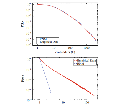
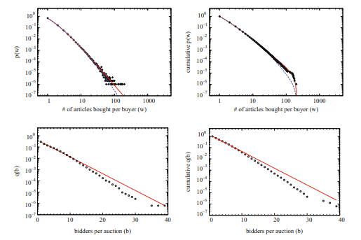
Prior to a block modeling analysis in this bidder network, we study its general statistical properties looking for indications of block structure [32]. We compare the results to a randomized null model (RNM) obtained from reshuffling the original data, i.e., keeping the attractiveness of each auction and the activity of each bidder constant, but randomizing which bidders take part in which auction. If the presence of clusters of users with a common interest has an influence on the statistical parameters of the network, it should be detectable by comparison with such a random null model. Figure 7.6 shows a comparison between the empirical data and the RNM in terms of the cumulative degree distribution, the cumulative distribution of the link weights as well as the clustering coefficient $c(k)$ as a function of the degree $k$.

数学代写|复杂网络代写complex networks代考|Network Clustering

The analysis of the user interests in the eBay market is based on the bidder network as constructed in the previous section. The links in this network represent articles the connected bidders (nodes) have a common interest in. The network is reduced to only those bidders that have taken part in at least two auctions and only auctions with a final price below 1,000 Euro are considered, thereby focussing on consumer goods. See Table 7.4 for the basic parameters of this reduced network.

If one now finds groups of users (clusters or communities [34-36]) with a high density of links among themselves and a low density of links to the rest of the network, the total set of links within such a group of users can be interpreted as a unifying common interest of this group. We fit a diagonal block model as introduced in Chap. 4. Recall the quality function $Q$ used:
$$
Q=\sum_s \underbrace{\left(m_{s s}-\gamma\left[m_{s s}\right]\right)}{c{s s}}=-\sum_{s<r} \underbrace{\left(m_{r s}-\gamma\left[m_{r s}\right]\right)}{a{r s}} .
$$
Note that any assignment of bidders into groups which maximizes $Q$ will be characterized by both maximum cohesion of groups and minimal adhesion between groups. If $Q$ is maximal, every node is classified in that group to which it has the largest adhesion. Compare Chap. 4 again for examples and further details of this quality function. Maximally 500 different groups of bidders were allowed in the analysis which gives a sufficient level of detail.
Figure 7.7 compares the results obtained with $\gamma=0.5$ and $\gamma=1$. Shown are the adjacency matrices $A_{i j}$ of the largest connected component of the bidder network. A black pixel at position $(i, j)$ and $(j, i)$ is shown on an $889,828 \times 889,828$ square if bidders $i$ and $j$ have competed in an auction and hence $A_{i j}=1$, otherwise the pixel is left white corresponding to $A_{i j}=0$. The rows and columns are ordered such that bidders who are classified as being in the same group are next to each other. The internal order of bidders within groups is random. The order of the groups was chosen to optimally show the correspondence between the ordering resulting from the $\gamma=0.5$ and the $\gamma=1$ ordering. In this representation, link densities correspond to pixel densities and thus to gray levels in the figure. Information about the exact size and link density contrast of the clusters is given in Table 7.5. Note the high contrast between internal and external link density.

数学代写|复杂网络代写complex networks代考|CS7280

数学代写|复杂网络代写complex networks代考|User Networks

从原始数据可以构造出许多市场网络。最自然的一种当然是由实际交易连接起来的用户网络。另一个是卖家网络,如果他们向同一用户销售产品,他们就会联系在一起。然后,网络中的链接将代表可能的竞争或合作的可能性,这取决于这些卖家提供的产品组合。这种情况也被称为“合作竞争”。同样,这种合作竞争网络也可以基于不同的卖家收到来自同一用户的出价这一事实来构建。此外,基于他们从同一卖家那里购买的事实来构建客户群体是可能的,这将再次定义加入这些客户的卖家的合作竞争情况。人们还可以研究文章或类别之间的关系,当它们收到来自同一用户的出价时,将它们加入网络。这将类似于频繁项目或频繁类别分析。

这里的重点是基于单篇文章的竞价网络。如果两个竞标者在拍卖中有过竞争,他们就会被联系在一起。由于在一次拍卖中出价的所有用户都是相互连接的,因此该网络是通过覆盖每次拍卖产生的完全连接的竞标者集团而形成的。这种图也被称为隶属网络[29-31]。注意,我们也可以根据竞标者见面的次数或根据他们出价的金额的某种函数来为竞标者之间的联系分配权重。
在对该投标人网络进行区块建模分析之前,我们研究了其一般统计特性,寻找区块结构的迹象[32]。我们将结果与通过重新洗牌原始数据获得的随机零模型(RNM)进行比较,即保持每次拍卖的吸引力和每个竞标者的活动不变,但随机选择竞标者参加哪种拍卖。如果具有共同兴趣的用户群的存在对网络的统计参数有影响,则应该通过与这种随机零模型进行比较来检测。图7.6显示了经验数据与RNM在累积度分布、链路权重累积分布以及聚类系数$c(k)$作为程度的函数$k$方面的比较。

数学代写|复杂网络代写complex networks代考|Network Clustering

对eBay市场中用户利益的分析是基于上一节所构建的投标人网络。该网络中的链接表示所连接的投标人(节点)有共同兴趣的物品。该网络只考虑那些参加过至少两次拍卖的投标人,并且只考虑最终价格低于1000欧元的拍卖,从而专注于消费品。该简化网络的基本参数见表7.4。

如果现在发现用户群(集群或社区[34-36])之间的链接密度很高,而与网络其他部分的链接密度很低,那么这样一组用户内的总链接集可以被解释为该组的统一共同利益。我们拟合了第4章中介绍的对角块模型。召回质量功能 $Q$ 使用:
$$
Q=\sum_s \underbrace{\left(m_{s s}-\gamma\left[m_{s s}\right]\right)}{c{s s}}=-\sum_{s<r} \underbrace{\left(m_{r s}-\gamma\left[m_{r s}\right]\right)}{a{r s}} .
$$
请注意,任何投标人分配到最大限度的组 $Q$ 将以群体之间最大的凝聚力和群体之间最小的粘连为特征。如果 $Q$ 如果是最大值,则每个节点都被分类到与其粘附最大的组中。再次比较第4章的例子和这个质量函数的进一步细节。最多500个不同的投标人组被允许在分析,给出了足够的细节水平。
图7.7将得到的结果与 $\gamma=0.5$ 和 $\gamma=1$. 所示为邻接矩阵 $A_{i j}$ 投标人网络中最大的连接组件。位置上的黑色像素 $(i, j)$ 和 $(j, i)$ 显示在 $889,828 \times 889,828$ 对竞标者进行清算 $i$ 和 $j$ 参加过拍卖,然后呢 $A_{i j}=1$,否则像素为左白对应 $A_{i j}=0$. 行和列的顺序是这样的竞标者被归类为在同一组是彼此相邻。组内竞标者的内部顺序是随机的。所选择的组的顺序是为了最佳地显示由的排序之间的对应关系 $\gamma=0.5$ 还有 $\gamma=1$ 订购。在这种表示中,链路密度对应于像素密度,从而对应于图中的灰度级。表7.5给出了关于集群的确切大小和链接密度对比的信息。注意内部和外部链接密度之间的高对比度。

统计代写|复杂网络代写complex networks代考 请认准statistics-lab™

统计代写请认准statistics-lab™. statistics-lab™为您的留学生涯保驾护航。统计代写|python代写代考

随机过程代考

在概率论概念中,随机过程随机变量的集合。 若一随机系统的样本点是随机函数,则称此函数为样本函数,这一随机系统全部样本函数的集合是一个随机过程。 实际应用中,样本函数的一般定义在时间域或者空间域。 随机过程的实例如股票和汇率的波动、语音信号、视频信号、体温的变化,随机运动如布朗运动、随机徘徊等等。

贝叶斯方法代考

贝叶斯统计概念及数据分析表示使用概率陈述回答有关未知参数的研究问题以及统计范式。后验分布包括关于参数的先验分布,和基于观测数据提供关于参数的信息似然模型。根据选择的先验分布和似然模型,后验分布可以解析或近似,例如,马尔科夫链蒙特卡罗 (MCMC) 方法之一。贝叶斯统计概念及数据分析使用后验分布来形成模型参数的各种摘要,包括点估计,如后验平均值、中位数、百分位数和称为可信区间的区间估计。此外,所有关于模型参数的统计检验都可以表示为基于估计后验分布的概率报表。

广义线性模型代考

广义线性模型(GLM)归属统计学领域,是一种应用灵活的线性回归模型。该模型允许因变量的偏差分布有除了正态分布之外的其它分布。

statistics-lab作为专业的留学生服务机构,多年来已为美国、英国、加拿大、澳洲等留学热门地的学生提供专业的学术服务,包括但不限于Essay代写,Assignment代写,Dissertation代写,Report代写,小组作业代写,Proposal代写,Paper代写,Presentation代写,计算机作业代写,论文修改和润色,网课代做,exam代考等等。写作范围涵盖高中,本科,研究生等海外留学全阶段,辐射金融,经济学,会计学,审计学,管理学等全球99%专业科目。写作团队既有专业英语母语作者,也有海外名校硕博留学生,每位写作老师都拥有过硬的语言能力,专业的学科背景和学术写作经验。我们承诺100%原创,100%专业,100%准时,100%满意。

机器学习代写

随着AI的大潮到来,Machine Learning逐渐成为一个新的学习热点。同时与传统CS相比,Machine Learning在其他领域也有着广泛的应用,因此这门学科成为不仅折磨CS专业同学的“小恶魔”,也是折磨生物、化学、统计等其他学科留学生的“大魔王”。学习Machine learning的一大绊脚石在于使用语言众多,跨学科范围广,所以学习起来尤其困难。但是不管你在学习Machine Learning时遇到任何难题,StudyGate专业导师团队都能为你轻松解决。

多元统计分析代考


基础数据: $N$ 个样本, $P$ 个变量数的单样本,组成的横列的数据表
变量定性: 分类和顺序;变量定量:数值
数学公式的角度分为: 因变量与自变量

时间序列分析代写

随机过程,是依赖于参数的一组随机变量的全体,参数通常是时间。 随机变量是随机现象的数量表现,其时间序列是一组按照时间发生先后顺序进行排列的数据点序列。通常一组时间序列的时间间隔为一恒定值(如1秒,5分钟,12小时,7天,1年),因此时间序列可以作为离散时间数据进行分析处理。研究时间序列数据的意义在于现实中,往往需要研究某个事物其随时间发展变化的规律。这就需要通过研究该事物过去发展的历史记录,以得到其自身发展的规律。

回归分析代写

多元回归分析渐进(Multiple Regression Analysis Asymptotics)属于计量经济学领域,主要是一种数学上的统计分析方法,可以分析复杂情况下各影响因素的数学关系,在自然科学、社会和经济学等多个领域内应用广泛。

MATLAB代写

MATLAB 是一种用于技术计算的高性能语言。它将计算、可视化和编程集成在一个易于使用的环境中,其中问题和解决方案以熟悉的数学符号表示。典型用途包括:数学和计算算法开发建模、仿真和原型制作数据分析、探索和可视化科学和工程图形应用程序开发,包括图形用户界面构建MATLAB 是一个交互式系统,其基本数据元素是一个不需要维度的数组。这使您可以解决许多技术计算问题,尤其是那些具有矩阵和向量公式的问题,而只需用 C 或 Fortran 等标量非交互式语言编写程序所需的时间的一小部分。MATLAB 名称代表矩阵实验室。MATLAB 最初的编写目的是提供对由 LINPACK 和 EISPACK 项目开发的矩阵软件的轻松访问,这两个项目共同代表了矩阵计算软件的最新技术。MATLAB 经过多年的发展,得到了许多用户的投入。在大学环境中,它是数学、工程和科学入门和高级课程的标准教学工具。在工业领域,MATLAB 是高效研究、开发和分析的首选工具。MATLAB 具有一系列称为工具箱的特定于应用程序的解决方案。对于大多数 MATLAB 用户来说非常重要,工具箱允许您学习应用专业技术。工具箱是 MATLAB 函数(M 文件)的综合集合,可扩展 MATLAB 环境以解决特定类别的问题。可用工具箱的领域包括信号处理、控制系统、神经网络、模糊逻辑、小波、仿真等。

R语言代写问卷设计与分析代写
PYTHON代写回归分析与线性模型代写
MATLAB代写方差分析与试验设计代写
STATA代写机器学习/统计学习代写
SPSS代写计量经济学代写
EVIEWS代写时间序列分析代写
EXCEL代写深度学习代写
SQL代写各种数据建模与可视化代写

数学代写|复杂网络代写complex networks代考|TSKS33

如果你也在 怎样代写复杂网络Complex Network 这个学科遇到相关的难题,请随时右上角联系我们的24/7代写客服。复杂网络Complex Network分析研究如何识别、描述、可视化和分析复杂网络。分析网络最突出的方法是使用Python库NetworkX,它为构造和绘制复杂的神经网络提供了一种突出的方法。

复杂网络Complex NetworkCNA研究和应用爆炸式增长的主要原因有两个因素:一是廉价而强大的计算机的可用性,使在数学、物理和社会科学方面受过高级培训的研究人员和科学家能够进行一流的研究;另一个因素是人类社会、行为、生物、金融和技术方面日益复杂。

statistics-lab™ 为您的留学生涯保驾护航 在代写复杂网络complex networks方面已经树立了自己的口碑, 保证靠谱, 高质且原创的统计Statistics代写服务。我们的专家在代写复杂网络complex networks方面经验极为丰富,各种代写复杂网络complex networks相关的作业也就用不着说。

数学代写|复杂网络代写complex networks代考|TSKS33

数学代写|复杂网络代写complex networks代考|Graphs with More than Two Clusters

After we have dealt with graphs containing only two clusters, we will now turn to the problem of networks with more than two clusters. While in the case of two clusters we could write the cavity equations for an arbitrary degree distribution, we were able to find a simple formulation for more than two clusters only for one special topology, the random Bethe lattice with three links per node, such that a cavity field is composed of combining only two messages. For graphs with a different topology, we will have to resort to a population dynamics algorithm to be described in the next section.

Let us first consider how to calculate the $\eta_{c w}^{i n}$ for general $q$. A message with $\tau=c+w$ non-zero entries will have one correct entry and $w$ wrong entries for $\tau$ types of nodes, while for $q-\tau$ types of nodes, it will have no correct entry but $w+1$ wrong entries. Hence we can write straightforwardly
$$
\begin{aligned}
& \eta_{1 w}^{i n}=p_{i n} \eta_{1 w}+\frac{\left(1-p_{i n}\right)}{q-1}\left(w \eta_{1 w}+(q-1-w) \eta_{0, w+1}\right), \
& \eta_{0 w}^{i n}=p_{i n} \eta_{0 w}+\frac{\left(1-p_{i n}\right)}{q-1}\left(w \eta_{1, w-1}+(q-1-w) \eta_{0, w}\right) .
\end{aligned}
$$
We see that this recovers the unclustered case if $\eta_{1 w}=\eta_{0, w+1}=\eta_\tau$.

For a Bethe lattice with exactly three links per node, we can write the cavity equations for the order parameters $\eta_{c w}$ for an arbitrary number of clusters as
$$
\begin{aligned}
& \eta_{1 w}=\sum_{c=0}^1 \sum_{\alpha=1-c}^{w-c}\left(\begin{array}{l}
w \
\alpha
\end{array}\right) \eta_{c, \alpha}^{i n} \eta_{1-c, w-\alpha}^{i n}+\left(\eta_{1 w}^{i n}\right)^2+2 \eta_{1 w}^{i n} \sum_{\alpha=1}^{q-1-w}\left(\begin{array}{c}
q-1-w \
\alpha
\end{array}\right) \eta_{1, w+\alpha}^{i n} \
& +\sum_{\alpha=1}^{q-1-w} \sum_{\beta=1}^{q-1-w-\alpha}\left(\begin{array}{c}
q-1-w \
\alpha
\end{array}\right)\left(\begin{array}{c}
q-1-w-\alpha \
\beta
\end{array}\right) \eta_{1, w+\alpha}^{i n} \eta_{1, w+\beta}^{i n}, \
& \eta_{0 w}=\sum_{\alpha=1}^{w-1}\left(\begin{array}{c}
w \
\alpha
\end{array}\right) \eta_{0, \alpha}^{i n} \eta_{0, w-\alpha}^{i n}+\left(\eta_{0 w}^{i n}\right)^2+2 \eta_{1 w}^{i n} \eta_{0 w}^{i n} \
& +2 \sum_{\alpha=1}^{q-1-w}\left(\begin{array}{c}
q-1-w \
\alpha
\end{array}\right)\left(\eta_{0 w}^{i n} \eta_{1, w+\alpha}^{i n}+\eta_{1 w}^{i n} \eta_{0, w+\alpha}^{i n}+\eta_{0 w}^{i n} \eta_{0, w+\alpha}^{i n}\right) \
& +\sum_{\alpha=1}^{q-1-w} \sum_{\beta=1}^{q-1-w-\alpha}\left(\begin{array}{c}
q-1-w \
\alpha
\end{array}\right)\left(\begin{array}{c}
q-1-w-\alpha \
\beta
\end{array}\right) \
& \times\left(\eta_{0, w+\alpha}^{i n} \eta_{1, w+\beta}^{i n}+\eta_{1, w+\alpha}^{i n} \eta_{0, w+\beta}^{i n}+\eta_{0, w+\alpha}^{i n} \eta_{0, w+\beta}^{i n}\right) . \
&
\end{aligned}
$$

数学代写|复杂网络代写complex networks代考|Bethe Lattice with k = 3

For a Bethe lattice with exactly three links per node, we can write the cavity equations for the order parameters $\eta_{c w}$ for an arbitrary number of clusters as
$$
\begin{aligned}
& \eta_{1 w}=\sum_{c=0}^1 \sum_{\alpha=1-c}^{w-c}\left(\begin{array}{l}
w \
\alpha
\end{array}\right) \eta_{c, \alpha}^{i n} \eta_{1-c, w-\alpha}^{i n}+\left(\eta_{1 w}^{i n}\right)^2+2 \eta_{1 w}^{i n} \sum_{\alpha=1}^{q-1-w}\left(\begin{array}{c}
q-1-w \
\alpha
\end{array}\right) \eta_{1, w+\alpha}^{i n} \
& +\sum_{\alpha=1}^{q-1-w} \sum_{\beta=1}^{q-1-w-\alpha}\left(\begin{array}{c}
q-1-w \
\alpha
\end{array}\right)\left(\begin{array}{c}
q-1-w-\alpha \
\beta
\end{array}\right) \eta_{1, w+\alpha}^{i n} \eta_{1, w+\beta}^{i n}, \
& \eta_{0 w}=\sum_{\alpha=1}^{w-1}\left(\begin{array}{c}
w \
\alpha
\end{array}\right) \eta_{0, \alpha}^{i n} \eta_{0, w-\alpha}^{i n}+\left(\eta_{0 w}^{i n}\right)^2+2 \eta_{1 w}^{i n} \eta_{0 w}^{i n} \
& +2 \sum_{\alpha=1}^{q-1-w}\left(\begin{array}{c}
q-1-w \
\alpha
\end{array}\right)\left(\eta_{0 w}^{i n} \eta_{1, w+\alpha}^{i n}+\eta_{1 w}^{i n} \eta_{0, w+\alpha}^{i n}+\eta_{0 w}^{i n} \eta_{0, w+\alpha}^{i n}\right) \
& +\sum_{\alpha=1}^{q-1-w} \sum_{\beta=1}^{q-1-w-\alpha}\left(\begin{array}{c}
q-1-w \
\alpha
\end{array}\right)\left(\begin{array}{c}
q-1-w-\alpha \
\beta
\end{array}\right) \
& \times\left(\eta_{0, w+\alpha}^{i n} \eta_{1, w+\beta}^{i n}+\eta_{1, w+\alpha}^{i n} \eta_{0, w+\beta}^{i n}+\eta_{0, w+\alpha}^{i n} \eta_{0, w+\beta}^{i n}\right) . \
&
\end{aligned}
$$
These equations must be read as describing the different ways and their probabilities in which two messages can be combined to form a cavity field and the resulting cavity bias. They can be iterated very easily to give the order parameters over the entire range of $p_{i n}$.

Figure 6.6 shows two examples for a three and a four partitioning of the Bethe lattice with three links per node. Note the similarity also to Fig. 6.4 and that $p_{i n}^c$ decreases slightly for increasing $q$. The qualitative behavior of the order parameters is the same across all degree distributions. Note how $\eta_{1, w-1}=\eta_{0, w}$ for all $p_{i n} \leq p_{i n}^c$ and $\eta_{1, w-1}>\eta_{0, w}$ for all $p_{i n}>p_{i n}^c$. Also note the different scales of the graphs, $\eta_{10}$ quickly starts to dominate all other order parameters.

数学代写|复杂网络代写complex networks代考|TSKS33

数学代写|复杂网络代写complex networks代考|Graphs with More than Two Clusters

在处理了仅包含两个簇的图之后,我们现在将转向包含两个以上簇的网络问题。虽然在两个簇的情况下,我们可以为任意度分布编写空腔方程,但我们能够为两个以上的簇找到一个简单的公式,只有一个特殊的拓扑,每个节点有三个链接的随机Bethe晶格,这样一个空腔场只由两个消息组合而成。对于具有不同拓扑结构的图,我们将不得不求助于种群动态算法,该算法将在下一节中描述。

让我们首先考虑如何计算一般的$q$的$\eta_{c w}^{i n}$。对于$\tau$类型的节点,具有$\tau=c+w$非零条目的消息将有一个正确条目和$w$错误条目,而对于$q-\tau$类型的节点,它将没有正确条目但有$w+1$错误条目。因此我们可以直接写出来
$$
\begin{aligned}
& \eta_{1 w}^{i n}=p_{i n} \eta_{1 w}+\frac{\left(1-p_{i n}\right)}{q-1}\left(w \eta_{1 w}+(q-1-w) \eta_{0, w+1}\right), \
& \eta_{0 w}^{i n}=p_{i n} \eta_{0 w}+\frac{\left(1-p_{i n}\right)}{q-1}\left(w \eta_{1, w-1}+(q-1-w) \eta_{0, w}\right) .
\end{aligned}
$$
我们看到,如果$\eta_{1 w}=\eta_{0, w+1}=\eta_\tau$,这将恢复未聚集的情况。

对于每个节点恰好有三个链接的贝特晶格,我们可以将任意数量簇的序参数$\eta_{c w}$的空腔方程写成
$$
\begin{aligned}
& \eta_{1 w}=\sum_{c=0}^1 \sum_{\alpha=1-c}^{w-c}\left(\begin{array}{l}
w \
\alpha
\end{array}\right) \eta_{c, \alpha}^{i n} \eta_{1-c, w-\alpha}^{i n}+\left(\eta_{1 w}^{i n}\right)^2+2 \eta_{1 w}^{i n} \sum_{\alpha=1}^{q-1-w}\left(\begin{array}{c}
q-1-w \
\alpha
\end{array}\right) \eta_{1, w+\alpha}^{i n} \
& +\sum_{\alpha=1}^{q-1-w} \sum_{\beta=1}^{q-1-w-\alpha}\left(\begin{array}{c}
q-1-w \
\alpha
\end{array}\right)\left(\begin{array}{c}
q-1-w-\alpha \
\beta
\end{array}\right) \eta_{1, w+\alpha}^{i n} \eta_{1, w+\beta}^{i n}, \
& \eta_{0 w}=\sum_{\alpha=1}^{w-1}\left(\begin{array}{c}
w \
\alpha
\end{array}\right) \eta_{0, \alpha}^{i n} \eta_{0, w-\alpha}^{i n}+\left(\eta_{0 w}^{i n}\right)^2+2 \eta_{1 w}^{i n} \eta_{0 w}^{i n} \
& +2 \sum_{\alpha=1}^{q-1-w}\left(\begin{array}{c}
q-1-w \
\alpha
\end{array}\right)\left(\eta_{0 w}^{i n} \eta_{1, w+\alpha}^{i n}+\eta_{1 w}^{i n} \eta_{0, w+\alpha}^{i n}+\eta_{0 w}^{i n} \eta_{0, w+\alpha}^{i n}\right) \
& +\sum_{\alpha=1}^{q-1-w} \sum_{\beta=1}^{q-1-w-\alpha}\left(\begin{array}{c}
q-1-w \
\alpha
\end{array}\right)\left(\begin{array}{c}
q-1-w-\alpha \
\beta
\end{array}\right) \
& \times\left(\eta_{0, w+\alpha}^{i n} \eta_{1, w+\beta}^{i n}+\eta_{1, w+\alpha}^{i n} \eta_{0, w+\beta}^{i n}+\eta_{0, w+\alpha}^{i n} \eta_{0, w+\beta}^{i n}\right) . \
&
\end{aligned}
$$

数学代写|复杂网络代写complex networks代考|Bethe Lattice with k = 3

对于每个节点恰好有三个链接的贝特晶格,我们可以将任意数量簇的序参数$\eta_{c w}$的空腔方程写成
$$
\begin{aligned}
& \eta_{1 w}=\sum_{c=0}^1 \sum_{\alpha=1-c}^{w-c}\left(\begin{array}{l}
w \
\alpha
\end{array}\right) \eta_{c, \alpha}^{i n} \eta_{1-c, w-\alpha}^{i n}+\left(\eta_{1 w}^{i n}\right)^2+2 \eta_{1 w}^{i n} \sum_{\alpha=1}^{q-1-w}\left(\begin{array}{c}
q-1-w \
\alpha
\end{array}\right) \eta_{1, w+\alpha}^{i n} \
& +\sum_{\alpha=1}^{q-1-w} \sum_{\beta=1}^{q-1-w-\alpha}\left(\begin{array}{c}
q-1-w \
\alpha
\end{array}\right)\left(\begin{array}{c}
q-1-w-\alpha \
\beta
\end{array}\right) \eta_{1, w+\alpha}^{i n} \eta_{1, w+\beta}^{i n}, \
& \eta_{0 w}=\sum_{\alpha=1}^{w-1}\left(\begin{array}{c}
w \
\alpha
\end{array}\right) \eta_{0, \alpha}^{i n} \eta_{0, w-\alpha}^{i n}+\left(\eta_{0 w}^{i n}\right)^2+2 \eta_{1 w}^{i n} \eta_{0 w}^{i n} \
& +2 \sum_{\alpha=1}^{q-1-w}\left(\begin{array}{c}
q-1-w \
\alpha
\end{array}\right)\left(\eta_{0 w}^{i n} \eta_{1, w+\alpha}^{i n}+\eta_{1 w}^{i n} \eta_{0, w+\alpha}^{i n}+\eta_{0 w}^{i n} \eta_{0, w+\alpha}^{i n}\right) \
& +\sum_{\alpha=1}^{q-1-w} \sum_{\beta=1}^{q-1-w-\alpha}\left(\begin{array}{c}
q-1-w \
\alpha
\end{array}\right)\left(\begin{array}{c}
q-1-w-\alpha \
\beta
\end{array}\right) \
& \times\left(\eta_{0, w+\alpha}^{i n} \eta_{1, w+\beta}^{i n}+\eta_{1, w+\alpha}^{i n} \eta_{0, w+\beta}^{i n}+\eta_{0, w+\alpha}^{i n} \eta_{0, w+\beta}^{i n}\right) . \
&
\end{aligned}
$$
这些方程必须被理解为描述两个信息可以组合形成空腔场和由此产生的空腔偏置的不同方式及其概率。它们可以很容易地迭代以给出整个$p_{i n}$范围内的顺序参数。

统计代写|复杂网络代写complex networks代考 请认准statistics-lab™

统计代写请认准statistics-lab™. statistics-lab™为您的留学生涯保驾护航。统计代写|python代写代考

随机过程代考

在概率论概念中,随机过程随机变量的集合。 若一随机系统的样本点是随机函数,则称此函数为样本函数,这一随机系统全部样本函数的集合是一个随机过程。 实际应用中,样本函数的一般定义在时间域或者空间域。 随机过程的实例如股票和汇率的波动、语音信号、视频信号、体温的变化,随机运动如布朗运动、随机徘徊等等。

贝叶斯方法代考

贝叶斯统计概念及数据分析表示使用概率陈述回答有关未知参数的研究问题以及统计范式。后验分布包括关于参数的先验分布,和基于观测数据提供关于参数的信息似然模型。根据选择的先验分布和似然模型,后验分布可以解析或近似,例如,马尔科夫链蒙特卡罗 (MCMC) 方法之一。贝叶斯统计概念及数据分析使用后验分布来形成模型参数的各种摘要,包括点估计,如后验平均值、中位数、百分位数和称为可信区间的区间估计。此外,所有关于模型参数的统计检验都可以表示为基于估计后验分布的概率报表。

广义线性模型代考

广义线性模型(GLM)归属统计学领域,是一种应用灵活的线性回归模型。该模型允许因变量的偏差分布有除了正态分布之外的其它分布。

statistics-lab作为专业的留学生服务机构,多年来已为美国、英国、加拿大、澳洲等留学热门地的学生提供专业的学术服务,包括但不限于Essay代写,Assignment代写,Dissertation代写,Report代写,小组作业代写,Proposal代写,Paper代写,Presentation代写,计算机作业代写,论文修改和润色,网课代做,exam代考等等。写作范围涵盖高中,本科,研究生等海外留学全阶段,辐射金融,经济学,会计学,审计学,管理学等全球99%专业科目。写作团队既有专业英语母语作者,也有海外名校硕博留学生,每位写作老师都拥有过硬的语言能力,专业的学科背景和学术写作经验。我们承诺100%原创,100%专业,100%准时,100%满意。

机器学习代写

随着AI的大潮到来,Machine Learning逐渐成为一个新的学习热点。同时与传统CS相比,Machine Learning在其他领域也有着广泛的应用,因此这门学科成为不仅折磨CS专业同学的“小恶魔”,也是折磨生物、化学、统计等其他学科留学生的“大魔王”。学习Machine learning的一大绊脚石在于使用语言众多,跨学科范围广,所以学习起来尤其困难。但是不管你在学习Machine Learning时遇到任何难题,StudyGate专业导师团队都能为你轻松解决。

多元统计分析代考


基础数据: $N$ 个样本, $P$ 个变量数的单样本,组成的横列的数据表
变量定性: 分类和顺序;变量定量:数值
数学公式的角度分为: 因变量与自变量

时间序列分析代写

随机过程,是依赖于参数的一组随机变量的全体,参数通常是时间。 随机变量是随机现象的数量表现,其时间序列是一组按照时间发生先后顺序进行排列的数据点序列。通常一组时间序列的时间间隔为一恒定值(如1秒,5分钟,12小时,7天,1年),因此时间序列可以作为离散时间数据进行分析处理。研究时间序列数据的意义在于现实中,往往需要研究某个事物其随时间发展变化的规律。这就需要通过研究该事物过去发展的历史记录,以得到其自身发展的规律。

回归分析代写

多元回归分析渐进(Multiple Regression Analysis Asymptotics)属于计量经济学领域,主要是一种数学上的统计分析方法,可以分析复杂情况下各影响因素的数学关系,在自然科学、社会和经济学等多个领域内应用广泛。

MATLAB代写

MATLAB 是一种用于技术计算的高性能语言。它将计算、可视化和编程集成在一个易于使用的环境中,其中问题和解决方案以熟悉的数学符号表示。典型用途包括:数学和计算算法开发建模、仿真和原型制作数据分析、探索和可视化科学和工程图形应用程序开发,包括图形用户界面构建MATLAB 是一个交互式系统,其基本数据元素是一个不需要维度的数组。这使您可以解决许多技术计算问题,尤其是那些具有矩阵和向量公式的问题,而只需用 C 或 Fortran 等标量非交互式语言编写程序所需的时间的一小部分。MATLAB 名称代表矩阵实验室。MATLAB 最初的编写目的是提供对由 LINPACK 和 EISPACK 项目开发的矩阵软件的轻松访问,这两个项目共同代表了矩阵计算软件的最新技术。MATLAB 经过多年的发展,得到了许多用户的投入。在大学环境中,它是数学、工程和科学入门和高级课程的标准教学工具。在工业领域,MATLAB 是高效研究、开发和分析的首选工具。MATLAB 具有一系列称为工具箱的特定于应用程序的解决方案。对于大多数 MATLAB 用户来说非常重要,工具箱允许您学习应用专业技术。工具箱是 MATLAB 函数(M 文件)的综合集合,可扩展 MATLAB 环境以解决特定类别的问题。可用工具箱的领域包括信号处理、控制系统、神经网络、模糊逻辑、小波、仿真等。

R语言代写问卷设计与分析代写
PYTHON代写回归分析与线性模型代写
MATLAB代写方差分析与试验设计代写
STATA代写机器学习/统计学习代写
SPSS代写计量经济学代写
EVIEWS代写时间序列分析代写
EXCEL代写深度学习代写
SQL代写各种数据建模与可视化代写

统计代写|复杂网络代写complex networks代考|PCS810

如果你也在 怎样代写复杂网络Complex Network 这个学科遇到相关的难题,请随时右上角联系我们的24/7代写客服。复杂网络Complex Network分析研究如何识别、描述、可视化和分析复杂网络。分析网络最突出的方法是使用Python库NetworkX,它为构造和绘制复杂的神经网络提供了一种突出的方法。

复杂网络Complex NetworkCNA研究和应用爆炸式增长的主要原因有两个因素:一是廉价而强大的计算机的可用性,使在数学、物理和社会科学方面受过高级培训的研究人员和科学家能够进行一流的研究;另一个因素是人类社会、行为、生物、金融和技术方面日益复杂。

statistics-lab™ 为您的留学生涯保驾护航 在代写复杂网络complex networks方面已经树立了自己的口碑, 保证靠谱, 高质且原创的统计Statistics代写服务。我们的专家在代写复杂网络complex networks方面经验极为丰富,各种代写复杂网络complex networks相关的作业也就用不着说。

统计代写|复杂网络代写complex networks代考|PCS810

统计代写|复杂网络代写complex networks代考|Choice of a Penalty Function and Null Model

We have introduced $p_{i j}$ as a penalty on the matching of missing links in $\mathbf{A}$ to links in B. As such, it can in principle take any form or value that may seem suitable. However, we have already hinted at the fact that $p_{i j}$ can also be interpreted as a probability. As such, it provides a random null model for the network under study. The quality functions (3.13), (3.13) and (3.15) then all compare distribution of links as found in the network for a given assignment of nodes into blocks to the expected link (weight) distribution if links (weight) were distributed independently of the assignment of nodes into blocks according to $p_{i j}$. Maximizing the quality functions (3.13), (3.13) and (3.15) hence means to find an assignment of nodes into blocks such that the number (weight) of edges in blocks deviates as strongly as possible from the expectation value due to the random null model.

Two exemplary choices of link distributions or random null models shall be illustrated. Both fulfill the constraint that $\sum_{i j} w_{i j} A_{i j}=\sum_{i j} p_{i j}$. The simplest choice is to assume every link equally probable with probability $p_{i j}=p$ independent from $i$ to $j$. Writing
$$
p_{i j}=p=\frac{\sum_{k l} w_{k l} A_{k l}}{N^2}
$$
leads naturally to
$$
\left[m_{r s}\right]_p=p n_r n_s,
$$
with $n_r$ and $n_s$ denoting the number of nodes in group $r$ and $s$, respectively.

统计代写|复杂网络代写complex networks代考|Cohesion and Adhesion

From the above considerations and to simplify further developments, the concepts of “cohesion” and “adhesion” are introduced. The coefficient of adhesion between groups $r$ and $s$ is defined as
$$
a_{r s}=m_{r s}-\gamma\left[m_{r s}\right]{p{i j}} .
$$
For $r=s$, we call $c_{s s}=a_{s s}$ the coefficient of “cohesion”. Two groups of nodes have a positive coefficient of adhesion, if they are connected by edges bearing more weight than expected from $p_{i j}$. We hence call a group cohesive, if its nodes are connected by edges bearing more weight than expected from $p_{i j}$. This allows for a shorthand form of (3.15) as $\mathcal{Q}=\frac{1}{2} \sum_{r s}\left|a_{r s}\right|$ and we see that the block model $\mathbf{B}$ has entries of one where $a_{r s}>0$. Remember that $a_{r s}$ depends on the global parameter $\gamma$ and the assumed penalty function $p_{i j}$. For $\gamma=1$ and the model $p_{i j}=\frac{k_i^{\text {out }} k_j^{\text {in }}}{M}$ one finds
$$
\sum_{r s} a_{r s}=\sum_r a_{r s}=\sum_s a_{r s}=0 .
$$
This means that when $\mathbf{B}$ is assigned from (3.15) there exists at least one entry of one and at least one entry of zero in every row and column of $\mathbf{B}$ (provided that the network is not complete or zero).

统计代写|复杂网络代写complex networks代考|PCS810

复杂网络代写

统计代写|复杂网络代写complex networks代考|Choice of a Penalty Function and Null Model

我们引入$p_{i j}$作为对$\mathbf{A}$中缺失链接与b中的链接匹配的惩罚。因此,原则上它可以采用任何看起来合适的形式或值。然而,我们已经暗示了$p_{i j}$也可以被解释为概率的事实。因此,它为所研究的网络提供了一个随机的零模型。然后,质量函数(3.13),(3.13)和(3.15)都将网络中发现的给定节点分配为块的链接分布与预期的链接(权重)分布进行比较,如果链接(权重)的分布独立于根据$p_{i j}$将节点分配为块。因此,最大化质量函数(3.13)、(3.13)和(3.15)意味着将节点分配到块中,使得块中边的数量(权重)尽可能强烈地偏离由于随机零模型而产生的期望值。

将举例说明链路分布或随机零模型的两个示例性选择。都满足$\sum_{i j} w_{i j} A_{i j}=\sum_{i j} p_{i j}$。最简单的选择是假设每个链接都是等概率的,概率$p_{i j}=p$独立于$i$到$j$。写作
$$
p_{i j}=p=\frac{\sum_{k l} w_{k l} A_{k l}}{N^2}
$$
自然会导致
$$
\left[m_{r s}\right]_p=p n_r n_s,
$$
其中$n_r$和$n_s$分别表示$r$和$s$组中的节点数。

统计代写|复杂网络代写complex networks代考|Cohesion and Adhesion

从上述考虑出发,为了简化进一步的发展,我们引入了“内聚”和“粘附”的概念。定义组间的粘附系数$r$和$s$为
$$
a_{r s}=m_{r s}-\gamma\left[m_{r s}\right]{p{i j}} .
$$
对于$r=s$,我们称$c_{s s}=a_{s s}$为“内聚”系数。如果两组节点通过比$p_{i j}$所期望的权重更大的边连接,则它们的粘附系数为正。因此,我们称一个群为内聚的,如果它的节点由比$p_{i j}$所期望的权重更大的边连接。这允许(3.15)的简写形式为$\mathcal{Q}=\frac{1}{2} \sum_{r s}\left|a_{r s}\right|$,我们看到块模型$\mathbf{B}$有一个条目,其中$a_{r s}>0$。请记住,$a_{r s}$依赖于全局参数$\gamma$和假定的惩罚函数$p_{i j}$。对于$\gamma=1$和模型$p_{i j}=\frac{k_i^{\text {out }} k_j^{\text {in }}}{M}$,可以找到
$$
\sum_{r s} a_{r s}=\sum_r a_{r s}=\sum_s a_{r s}=0 .
$$
这意味着当从(3.15)中分配$\mathbf{B}$时,在$\mathbf{B}$的每一行和每一列中至少存在一个1和至少一个0的条目(前提是网络不完整或为零)。

统计代写|复杂网络代写complex networks代考 请认准statistics-lab™

统计代写请认准statistics-lab™. statistics-lab™为您的留学生涯保驾护航。统计代写|python代写代考

随机过程代考

在概率论概念中,随机过程随机变量的集合。 若一随机系统的样本点是随机函数,则称此函数为样本函数,这一随机系统全部样本函数的集合是一个随机过程。 实际应用中,样本函数的一般定义在时间域或者空间域。 随机过程的实例如股票和汇率的波动、语音信号、视频信号、体温的变化,随机运动如布朗运动、随机徘徊等等。

贝叶斯方法代考

贝叶斯统计概念及数据分析表示使用概率陈述回答有关未知参数的研究问题以及统计范式。后验分布包括关于参数的先验分布,和基于观测数据提供关于参数的信息似然模型。根据选择的先验分布和似然模型,后验分布可以解析或近似,例如,马尔科夫链蒙特卡罗 (MCMC) 方法之一。贝叶斯统计概念及数据分析使用后验分布来形成模型参数的各种摘要,包括点估计,如后验平均值、中位数、百分位数和称为可信区间的区间估计。此外,所有关于模型参数的统计检验都可以表示为基于估计后验分布的概率报表。

广义线性模型代考

广义线性模型(GLM)归属统计学领域,是一种应用灵活的线性回归模型。该模型允许因变量的偏差分布有除了正态分布之外的其它分布。

statistics-lab作为专业的留学生服务机构,多年来已为美国、英国、加拿大、澳洲等留学热门地的学生提供专业的学术服务,包括但不限于Essay代写,Assignment代写,Dissertation代写,Report代写,小组作业代写,Proposal代写,Paper代写,Presentation代写,计算机作业代写,论文修改和润色,网课代做,exam代考等等。写作范围涵盖高中,本科,研究生等海外留学全阶段,辐射金融,经济学,会计学,审计学,管理学等全球99%专业科目。写作团队既有专业英语母语作者,也有海外名校硕博留学生,每位写作老师都拥有过硬的语言能力,专业的学科背景和学术写作经验。我们承诺100%原创,100%专业,100%准时,100%满意。

机器学习代写

随着AI的大潮到来,Machine Learning逐渐成为一个新的学习热点。同时与传统CS相比,Machine Learning在其他领域也有着广泛的应用,因此这门学科成为不仅折磨CS专业同学的“小恶魔”,也是折磨生物、化学、统计等其他学科留学生的“大魔王”。学习Machine learning的一大绊脚石在于使用语言众多,跨学科范围广,所以学习起来尤其困难。但是不管你在学习Machine Learning时遇到任何难题,StudyGate专业导师团队都能为你轻松解决。

多元统计分析代考


基础数据: $N$ 个样本, $P$ 个变量数的单样本,组成的横列的数据表
变量定性: 分类和顺序;变量定量:数值
数学公式的角度分为: 因变量与自变量

时间序列分析代写

随机过程,是依赖于参数的一组随机变量的全体,参数通常是时间。 随机变量是随机现象的数量表现,其时间序列是一组按照时间发生先后顺序进行排列的数据点序列。通常一组时间序列的时间间隔为一恒定值(如1秒,5分钟,12小时,7天,1年),因此时间序列可以作为离散时间数据进行分析处理。研究时间序列数据的意义在于现实中,往往需要研究某个事物其随时间发展变化的规律。这就需要通过研究该事物过去发展的历史记录,以得到其自身发展的规律。

回归分析代写

多元回归分析渐进(Multiple Regression Analysis Asymptotics)属于计量经济学领域,主要是一种数学上的统计分析方法,可以分析复杂情况下各影响因素的数学关系,在自然科学、社会和经济学等多个领域内应用广泛。

MATLAB代写

MATLAB 是一种用于技术计算的高性能语言。它将计算、可视化和编程集成在一个易于使用的环境中,其中问题和解决方案以熟悉的数学符号表示。典型用途包括:数学和计算算法开发建模、仿真和原型制作数据分析、探索和可视化科学和工程图形应用程序开发,包括图形用户界面构建MATLAB 是一个交互式系统,其基本数据元素是一个不需要维度的数组。这使您可以解决许多技术计算问题,尤其是那些具有矩阵和向量公式的问题,而只需用 C 或 Fortran 等标量非交互式语言编写程序所需的时间的一小部分。MATLAB 名称代表矩阵实验室。MATLAB 最初的编写目的是提供对由 LINPACK 和 EISPACK 项目开发的矩阵软件的轻松访问,这两个项目共同代表了矩阵计算软件的最新技术。MATLAB 经过多年的发展,得到了许多用户的投入。在大学环境中,它是数学、工程和科学入门和高级课程的标准教学工具。在工业领域,MATLAB 是高效研究、开发和分析的首选工具。MATLAB 具有一系列称为工具箱的特定于应用程序的解决方案。对于大多数 MATLAB 用户来说非常重要,工具箱允许您学习应用专业技术。工具箱是 MATLAB 函数(M 文件)的综合集合,可扩展 MATLAB 环境以解决特定类别的问题。可用工具箱的领域包括信号处理、控制系统、神经网络、模糊逻辑、小波、仿真等。

R语言代写问卷设计与分析代写
PYTHON代写回归分析与线性模型代写
MATLAB代写方差分析与试验设计代写
STATA代写机器学习/统计学习代写
SPSS代写计量经济学代写
EVIEWS代写时间序列分析代写
EXCEL代写深度学习代写
SQL代写各种数据建模与可视化代写