如果你也在 怎样代写固体物理Solid-state physics这个学科遇到相关的难题，请随时右上角联系我们的24/7代写客服。

固态物理学是通过量子力学、晶体学、电磁学和冶金学等方法研究刚性物质或固体。它是凝聚态物理学的最大分支。

statistics-lab™ 为您的留学生涯保驾护航 在代写固体物理Solid-state physics方面已经树立了自己的口碑, 保证靠谱, 高质且原创的统计Statistics代写服务。我们的专家在代写固体物理Solid-state physics代写方面经验极为丰富，各种代写固体物理Solid-state physics相关的作业也就用不着说。

我们提供的固体物理Solid-state physics及其相关学科的代写，服务范围广, 其中包括但不限于:

• Statistical Inference 统计推断
• Statistical Computing 统计计算
• Advanced Probability Theory 高等概率论
• Advanced Mathematical Statistics 高等数理统计学
• (Generalized) Linear Models 广义线性模型
• Statistical Machine Learning 统计机器学习
• Longitudinal Data Analysis 纵向数据分析
• Foundations of Data Science 数据科学基础

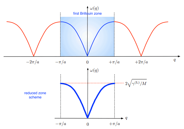
物理代写|固体物理代写Solid-state physics代考|Diatomic linear chain

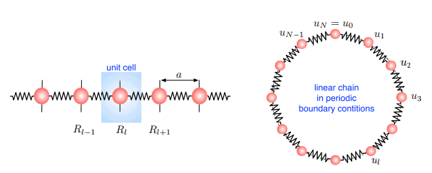
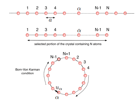
Let us now turn to consider the one-dimensional model of minimal complexity for a lattice with a basis, namely a diatomic linear chain. We need to define two ion masses $M_1$ and $M_2$ and two effective springs $\gamma^{(L)}$ and $\xi^{(L)}$, respectively, coupling ions within the same unit cell or belonging to nearest neighbouring unit cells. Ion positions are now indicated as $R_{l, 1}=R_l+R_1$ and $R_{l, 2}=R_l+R_2$, where $R_l$ labels the lth unit cell, while $R_1$ and $R_2$ specify the ion within the basis. The situation is sketched in figure $3.4$ and once again we start by considering longitudinal oscillations.

The equations of motion for the two ions in the lth unit cell form a system of two differential equations
$$
\left{\begin{array}{l}
M_1 \ddot{u}{l, 1}=\gamma^{(L)}\left(u{l, 2}-u_{l, 1}\right)+\xi^{(L)}\left(u_{l-1,2}-u_{l, 1}\right) \
M_2 \ddot{u}{l, 2}=\xi^{(L)}\left(u{l+1,1}-u_{l, 2}\right)+\gamma^{(L)}\left(u_{l, 1}-u_{l, 2}\right),
\end{array}\right.
$$
We seek solutions for this system of the same form given in equation (3.10). However, for further convenience, it is useful to rewrite the amplitude as $\left|\mathcal{A}q\right| \rightarrow\left|\mathcal{A}_q\right|\left|\mathrm{a}_i(q)\right|$ and the phase as $\varphi(q) \rightarrow \varphi(q)+\phi_i(q)$ (where $i=1,2$ labels the ion within the basis) since, as we will prove soon, the terms $\left|a_i(q)\right|$ and $\phi_i(q)$ are determined by the very equations of motion, rather than by the boundary conditions as instead $\left|\mathcal{A}_q\right|$ and $\varphi(q)$. By this choice, we write $$ u{l, i}=\frac{1}{\sqrt{N M_i}} \sum_q\left|\mathcal{A}q\right|\left|a_i(q)\right| \cos \left[q R{l, i}-\omega(q) t+\varphi(q)+\phi_i(q)\right],
$$
which, if inserted in equations (3.11), leads to the following matrix equation
$$
\left(\begin{array}{ll}
\mathcal{D}{11} & \mathcal{D}{12} \
\mathcal{D}{21} & \mathcal{D}{22}
\end{array}\right)\left(\begin{array}{l}
a_1 \
a_2
\end{array}\right)=\omega^2\left(\begin{array}{l}
a_1 \
a_2
\end{array}\right),
$$

物理代写|固体物理代写Solid-state physics代考|Dynamics of three-dimensional crystals

The dynamical properties of a three-dimensional solid with arbitrary crystalline structure or basis configuration can only be described by means of a heavy formalism $[5,6,8]$, which somewhat hides the underlying physics. This is the pedagogical reason why we have preliminarily treated the model system corresponding to a linear chain: we will extensively make use of concepts developed in that framework. As for the formal procedures, we will instead follow the same line of action adopted in section 3.1. In particular, we will assume that a suitable force field describing the interactions among ions is available (see appendix D); once for all, therefore, the force constants defined in equation (3.2) are given as known. More important, however, is the fact that we will rely on the harmonic approximation.
Before starting to develop our theory, we preliminarily remark that in a threedimensional crystal containing $N_{\text {atom }}$ atoms in its unit cell, we have $3 N_{\text {atom }}$ ionic degrees of freedom (per unit cell) and, therefore, an equal number of branches in the vibrational dispersion relations; among them we will find 3 acoustic and $3\left(N_{\text {atom }}-1\right)$ optical branches.
In the harmonic approximation, the equations of motion are written as ${ }^9$
$$
M_b \ddot{u}i(l b)=-\sum{j l^{\prime} b^{\prime}} U_{i j}\left(l b, l^{\prime} b^{\prime}\right) u_j\left(l^{\prime} b^{\prime}\right),
$$
for which we guess solutions in the form
$$
u_i(l b)=\frac{\mathrm{a}_i(b \mid \mathbf{q})}{\sqrt{M_b}} e^{i q \cdot \mathbf{R}_i} e^{-i \omega t},
$$
where $M_b$ is the mass of the $b$ th ion in the basis ${ }^{10}, \mathbf{q}$ is the wavevector of the vibrational wave and $a_i(b \mid q)$ describes the amplitude of the corresponding ionic oscillations. By inserting this guessed displacement into the equations of motion we get
$$
\sum_{j b^{\prime}} \mathcal{D}{i j}\left(b b^{\prime} \mid \mathbf{q}\right) a_j\left(b^{\prime} \mid \mathbf{q}\right)=\omega^2 a_i(b \mid \mathbf{q}) $$ where the quantities $$ \mathcal{D}{i j}\left(b b^{\prime} \mid \mathbf{q}\right)=\frac{1}{\sqrt{M_b M_{b^{\prime}}}} \sum_{l^{\prime}} U_{i j}\left(l b, l^{\prime} b^{\prime}\right) e^{-i \mathbf{q} \cdot\left(\mathbf{R}l-\mathbf{R}_r\right)} $$ define the dynamical matrix of the crystal. It is important to remark that in this equation just a single summation of the cell index $l^{\prime}$ appears since the force constants $U{i j}\left(l b, l^{\prime} b^{\prime}\right)$ of an ideal crystal depend on the pair $\left(l, l^{\prime}\right)$ just through their difference ${ }^{11}$. This also reflects the choice of the guessed solution for the ionic displacements in the form of a Bloch wave.

固体物理代写

物理代写|固体物理代写Solid-state physics代考|Diatomic linear chain

现在让我们转向考虑具有基的晶格的最小复杂度的一维模型，即双原子线性链。我们需要定义两个离子质量 $M_1$ 和 $M_2$ 和两个有效弹簧 $\gamma^{(L)}$ 和 $\xi^{(L)}$ ，分别耦合同一晶胞内或属于最近的相邻晶胞的离子。离子位置现在表示为 $R_{l, 1}=R_l+R_1$ 和 $R_{l, 2}=R_l+R_2$ ，在哪里 $R_l$ 标记第 $\mathrm{个}$ 个晶胞，而 $R_1$ 和 $R_2$ 指定基内的离子。情况如图 $3.4$ 我们再次从考虑纵向振荡开始。
第 |个晶胞中两个离子的运动方程形成了一个由两个微分方程组成的系统
$\$ \$$
Veft {
$M_1 \ddot{u} l, 1=\gamma^{(L)}\left(u l, 2-u_{l, 1}\right)+\xi^{(L)}\left(u_{l-1,2}-u_{l, 1}\right) M_2 \ddot{u} l, 2=\xi^{(L)}\left(u l+1,1-u_{l, 2}\right)+\gamma^{(L)}\left(u_{l, 1}-u_{l, 2}\right)$
【正确的。
Weseeksolutions forthissystemofthesame formgiveninequation (3.10). However, for furthercon $\mathrm{t}+$ Ivarphi(q)+\phi_i(q)\right],
which, ifinsertedinequations(3.11), leadstothe followingmatrixequation
剩下（
$\begin{array}{llll}\mathcal{D} 11 & \mathcal{D} 12 & \mathcal{D} 21 & \mathcal{D} 22\end{array}$
右左 (
$a_1 a_2$
Iright)=lomega^2lleft(
$a_1 a_2$
右），
$\$ \$$

物理代写|固体物理代写Solid-state physics代考|Dynamics of three-dimensional crystals

具有任意晶体结构或基本构型的三维固体的动力学性质只能通过繁重的形式来描述 $[5,6,8]$ ，这在某种程度上隐藏 了基础物理。这就是我们初步处理对应于线性链的模型系统的教学原因: 我们将广泛使用在该框架中开发的概
念。至于正式程序，我们将遵循第 $3.1$ 节中采用的相同行动路线。特别是，我们将假设描述离子间相互作用的合 适的力场是可用的 (见附录 D) ；因此，等式 (3.2) 中定义的力常数是已知的。然而，更重要的是我们将依赖诣波 近似。
在开始发展我们的理论之前，我们首先注意到在三维晶体中包含 $N_{\text {atom }}$ 晶胞中的原子，我们有 $3 N_{\text {atom 离子自由 }}$ 度 (每个晶胞) ，因此，振动色散关系中的分支数量相等；其中我们会发现 3 个声学和 $3\left(N_{\text {atom }}-1\right)$ 光学分 支。
在谐波近似中，运动方程写为 ${ }^9$
$\$ \$$
forwhichweguesssolutionsinthe form
where $\$ M_b \$$ isthemassofthe $\$ b \$$ thioninthebasis $\$^{10}, \mathbf{q}$ isthewavevectorofthevibrationalwaveand mathbf ${q} \backslash$ right $)=\backslash o m e g a^{\wedge} 2 a_{-} i(b \backslash m i d \backslash$ mathbf ${q})$
wherethequantities
Imathbf{R}_rıright $)} \$ \$$ 定义了晶体的动力学矩阵。重要的是要注意，在这个等式中只有一个细胞指数的总和 $l^{\prime}$ 由 于力常数出现 $U i j\left(l b, l^{\prime} b^{\prime}\right)$ 理想晶体的大小取决于对 $\left(l, l^{\prime}\right)$ 只是通过他们的不同 ${ }^{11}$. 这也反映了对布洛赫波形式的 离子位移的猜测解的选择。

统计代写请认准statistics-lab™. statistics-lab™为您的留学生涯保驾护航。

金融工程代写

金融工程是使用数学技术来解决金融问题。金融工程使用计算机科学、统计学、经济学和应用数学领域的工具和知识来解决当前的金融问题，以及设计新的和创新的金融产品。

非参数统计代写

非参数统计指的是一种统计方法，其中不假设数据来自于由少数参数决定的规定模型；这种模型的例子包括正态分布模型和线性回归模型。

广义线性模型代考

广义线性模型（GLM）归属统计学领域，是一种应用灵活的线性回归模型。该模型允许因变量的偏差分布有除了正态分布之外的其它分布。

术语 广义线性模型（GLM）通常是指给定连续和/或分类预测因素的连续响应变量的常规线性回归模型。它包括多元线性回归，以及方差分析和方差分析（仅含固定效应）。

有限元方法代写

有限元方法（FEM）是一种流行的方法，用于数值解决工程和数学建模中出现的微分方程。典型的问题领域包括结构分析、传热、流体流动、质量运输和电磁势等传统领域。

有限元是一种通用的数值方法，用于解决两个或三个空间变量的偏微分方程（即一些边界值问题）。为了解决一个问题，有限元将一个大系统细分为更小、更简单的部分，称为有限元。这是通过在空间维度上的特定空间离散化来实现的，它是通过构建对象的网格来实现的：用于求解的数值域，它有有限数量的点。边界值问题的有限元方法表述最终导致一个代数方程组。该方法在域上对未知函数进行逼近。[1] 然后将模拟这些有限元的简单方程组合成一个更大的方程系统，以模拟整个问题。然后，有限元通过变化微积分使相关的误差函数最小化来逼近一个解决方案。

tatistics-lab作为专业的留学生服务机构，多年来已为美国、英国、加拿大、澳洲等留学热门地的学生提供专业的学术服务，包括但不限于Essay代写，Assignment代写，Dissertation代写，Report代写，小组作业代写，Proposal代写，Paper代写，Presentation代写，计算机作业代写，论文修改和润色，网课代做，exam代考等等。写作范围涵盖高中，本科，研究生等海外留学全阶段，辐射金融，经济学，会计学，审计学，管理学等全球99%专业科目。写作团队既有专业英语母语作者，也有海外名校硕博留学生，每位写作老师都拥有过硬的语言能力，专业的学科背景和学术写作经验。我们承诺100%原创，100%专业，100%准时，100%满意。

随机分析代写

随机微积分是数学的一个分支，对随机过程进行操作。它允许为随机过程的积分定义一个关于随机过程的一致的积分理论。这个领域是由日本数学家伊藤清在第二次世界大战期间创建并开始的。

时间序列分析代写

随机过程，是依赖于参数的一组随机变量的全体，参数通常是时间。 随机变量是随机现象的数量表现，其时间序列是一组按照时间发生先后顺序进行排列的数据点序列。通常一组时间序列的时间间隔为一恒定值（如1秒，5分钟，12小时，7天，1年），因此时间序列可以作为离散时间数据进行分析处理。研究时间序列数据的意义在于现实中，往往需要研究某个事物其随时间发展变化的规律。这就需要通过研究该事物过去发展的历史记录，以得到其自身发展的规律。

回归分析代写

多元回归分析渐进（Multiple Regression Analysis Asymptotics）属于计量经济学领域，主要是一种数学上的统计分析方法，可以分析复杂情况下各影响因素的数学关系，在自然科学、社会和经济学等多个领域内应用广泛。

MATLAB代写

MATLAB 是一种用于技术计算的高性能语言。它将计算、可视化和编程集成在一个易于使用的环境中，其中问题和解决方案以熟悉的数学符号表示。典型用途包括：数学和计算算法开发建模、仿真和原型制作数据分析、探索和可视化科学和工程图形应用程序开发，包括图形用户界面构建MATLAB 是一个交互式系统，其基本数据元素是一个不需要维度的数组。这使您可以解决许多技术计算问题，尤其是那些具有矩阵和向量公式的问题，而只需用 C 或 Fortran 等标量非交互式语言编写程序所需的时间的一小部分。MATLAB 名称代表矩阵实验室。MATLAB 最初的编写目的是提供对由 LINPACK 和 EISPACK 项目开发的矩阵软件的轻松访问，这两个项目共同代表了矩阵计算软件的最新技术。MATLAB 经过多年的发展，得到了许多用户的投入。在大学环境中，它是数学、工程和科学入门和高级课程的标准教学工具。在工业领域，MATLAB 是高效研究、开发和分析的首选工具。MATLAB 具有一系列称为工具箱的特定于应用程序的解决方案。对于大多数 MATLAB 用户来说非常重要，工具箱允许您学习和应用专业技术。工具箱是 MATLAB 函数（M 文件）的综合集合，可扩展 MATLAB 环境以解决特定类别的问题。可用工具箱的领域包括信号处理、控制系统、神经网络、模糊逻辑、小波、仿真等。

R语言代写	问卷设计与分析代写
PYTHON代写	回归分析与线性模型代写
MATLAB代写	方差分析与试验设计代写
STATA代写	机器学习/统计学习代写
SPSS代写	计量经济学代写
EVIEWS代写	时间序列分析代写
EXCEL代写	深度学习代写
SQL代写	各种数据建模与可视化代写

如果你也在 怎样代写固体物理Solid-state physics这个学科遇到相关的难题，请随时右上角联系我们的24/7代写客服。

固态物理学是通过量子力学、晶体学、电磁学和冶金学等方法研究刚性物质或固体。它是凝聚态物理学的最大分支。

statistics-lab™ 为您的留学生涯保驾护航 在代写固体物理Solid-state physics方面已经树立了自己的口碑, 保证靠谱, 高质且原创的统计Statistics代写服务。我们的专家在代写固体物理Solid-state physics代写方面经验极为丰富，各种代写固体物理Solid-state physics相关的作业也就用不着说。

我们提供的固体物理Solid-state physics及其相关学科的代写，服务范围广, 其中包括但不限于:

• Statistical Inference 统计推断
• Statistical Computing 统计计算
• Advanced Probability Theory 高等概率论
• Advanced Mathematical Statistics 高等数理统计学
• (Generalized) Linear Models 广义线性模型
• Statistical Machine Learning 统计机器学习
• Longitudinal Data Analysis 纵向数据分析
• Foundations of Data Science 数据科学基础

物理代写|固体物理代写Solid-state physics代考|Conceptual layout

The description of crystal structures developed in chapter 2 relies on an implicit (but really very strong) assumption, namely! ions are clamped at their lattice positions. This is, also, the situation assumed to define the eigenvalue problem for the total electron wavefunction given in equation (1.15) within the framework developed under the adiabatic approximation. While the assumption of static lattice is useful in the above contexts, it is either conceptually wrong and inadequate to describe many important solid state phenomena.

First of all, we recall that ions, although comparatively much more massive than electrons, have in fact a finite mass: therefore, according to fundamental quantum mechanics [1-4], they always (even at zero temperature) have a non-vanishing mean square momentum. We can reconcile crystallography with the quantum uncertainty principle by assuming that the mean position of an ion (obtained by averaging over its zero-point motion) corresponds to $\mathbf{R}1$ in Bravais lattices or to $\mathbf{R}_1+\mathbf{R}{\mathrm{b}}$ for lattices with a basis (see equations (2.1) and (2.3), respectively).

This is not enough. Still considering ions at rest (although in some ‘average’ meaning) is inconsistent with a number of experimental evidences, including (but not limited to): thermal expansion, melting, thermal conductivity, sound propagation, inelastic scattering of electromagnetic waves or particles (electrons as well as neutrons). All together these phenomena provide a robust body of experimental evidence that lattice ions do undergo some kind of motion. The aim of this chapter is to fully characterise the corresponding lattice dynamics.

We will accomplish this task at first under the leading adiabatic and classical approximations (see sections 1.3.4 and 1.4.2, respectively). Non-classical dynamical features will appear later, by a suitable quantisation procedure operated on the ionic classical displacement field. In developing our classical phenomenological theory of lattice dynamics, we will assume that there exists a many-body potential energy $U=U(\mathbf{R})$ governing the motion of the ions ${ }^1$. Basically, $U$ contains the ion-ion Coulomb interaction energy as well as their kinetic energy, as conceptualised in section 1.3.4.

物理代写|固体物理代写Solid-state physics代考|Monoatomic linear chain

Let us consider a linear chain where $N$ identical ions of mass $M$ are placed at distance $a$ when they are at rest in equilibrium positions. This corresponds to a onedimensional Bravais crystal with lattice spacing $a$; the primitive unit cell is obtained by the Wigner-Seitz construction as a segment of length $a$ with the ion placed at its midpoint. By adopting Born-von Karman boundary conditions, the ionic positions are indicated as $R_l=l a$ with $l=0,1,2, \ldots, N-1$. Finally, following the force constant approach discussed in the previous section, we represent the interactions between nearest neighbouring ions as harmonic springs. The situation is sketched in figure $3.1$.

Let us consider a longitudinal vibration of the chain, that is a displacement pattern in which the ions move along the chain direction. The classical equation of motion for the lth ion is
$$
M \ddot{u}l=\gamma^{(L)}\left(u{l+1}+u_{l-1}-2 u_l\right),
$$

where $\gamma^{(L)}$ is the force constant of the effective spring. Suggested by the elementary mechanics of a vibrating wire, we seek a solution in the form
$$
u_l=\frac{1}{\sqrt{N M}}\left|\mathcal{A}_q\right| \cos \left[q R_l-\omega(q) t+\varphi(q)\right],
$$
where the normalising factor $(N M)^{-1 / 2}$ has been introduced for further convenience, while $\left|\mathcal{A}_q\right|$ and $\varphi(q)$ are the amplitude and the initial phase of the wave ${ }^6$. Of course, $q$ and $\omega(q)$ are the wavenumber and the angular frequency of the travelling wave, respectively. Replacing equation (3.7) into equation (3.6) leads to
$$
M \omega^2(q)=2 \gamma^{(L)}[1-\cos (q a)]=4 \gamma^{(L)} \sin ^2\left(\frac{1}{2} q a\right),
$$
which is known as the dispersion relation and it is shown in figure 3.2(top). This representation is redundant since it ignores translational periodicity: it makes no difference in the displacement $u_l$ by increasing $q \rightarrow q+G$ with $G=2 m \pi / a$ a reciprocal lattice vector of the linear chain crystal ( $m$ is any positive or negative integer number). It is therefore customary to adopt the reduced zone scheme: the dispersion relation is represented only for $q \in 1 \mathrm{BZ}$ or, equivalently, for $q \in[-\pi / a,+\pi / a]$ as shown in figure 3.2(bottom). The actual number of allowed $q$ is determined by the imposed boundary conditions: since it must be $u_0=u_N$ then
$$
q=\frac{2 \pi}{a} \frac{\xi}{N} \quad \text { with } \quad \xi=0,1,2,3, \ldots, N-1
$$

固体物理代写

物理代写|固体物理代写Solid-state physics代考|Conceptual layout

第 2 章中对晶体结构的描述依赖于一个隐含的（但非常强的）假设，即！离子被夹在它们的晶格位置。这也是假定在绝热近似下发展的框架内定义方程（1.15）中给出的总电子波函数的特征值问题的情况。虽然静态晶格的假设在上述情况下很有用，但它要么在概念上是错误的，要么不足以描述许多重要的固态现象。

首先，我们回想起离子，虽然相对比电子大得多，但实际上具有有限的质量：因此，根据基本量子力学 [1-4]，它们总是（即使在零温度下）具有不消失的均方动量。我们可以通过假设离子的平均位置（通过在其零点运动上平均获得）对应于R1在 Bravais 格子中或R1+Rb对于有基础的晶格（分别参见方程（2.1）和（2.3））。

这还不够。仍然考虑静止的离子（尽管在某些“平均”意义上）与许多实验证据不一致，包括（但不限于）：热膨胀、熔化、导热性、声音传播、电磁波或粒子的非弹性散射（电子和中子）。所有这些现象共同提供了大量的实验证据，表明晶格离子确实经历了某种运动。本章的目的是充分表征相应的晶格动力学。

我们将首先在领先的绝热近似和经典近似下完成这项任务（分别参见第 1.3.4 节和第 1.4.2 节）。稍后将通过在离子经典位移场上操作的适当量化程序出现非经典动力学特征。在发展我们经典的晶格动力学唯象理论时，我们将假设存在多体势能在=在(R)控制离子的运动1. 基本上，在包含离子-离子库仑相互作用能以及它们的动能，如第 1.3.4 节所述。

物理代写|固体物理代写Solid-state physics代考|Monoatomic linear chain

让我们考虑一个线性链，其中 $N$ 质量相同的离子 $M$ 被放置在远处 $a$ 当它们静止在平衡位置时。这对应于具有晶格 间距的一维布拉维晶体 $a$; 原始晶胞是通过 Wigner-Seitz 构造获得的，作为一段长度 $a$ 离子位于其中点。通过采用 Born-von Karman 边界条件，离子位置表示为 $R_l=l a$ 和 $l=0,1,2, \ldots, N-1$. 最后，按照上一节中讨论的 力常数方法，我们将最近相邻离子之间的相互作用表示为谐波弹簧。情况如图3.1.
让我们考虑链的纵向振动，即离子沿链方向移动的位移模式。第 |个离子的经典运动方程是
$$
M \ddot{u} l=\gamma^{(L)}\left(u l+1+u_{l-1}-2 u_l\right),
$$
在哪里 $\gamma^{(L)}$ 是有效弹簧的力常数。由振弦的基本力学建议，我们寻求以下形式的解决方案
$$
u_l=\frac{1}{\sqrt{N M}}\left|\mathcal{A}_q\right| \cos \left[q R_l-\omega(q) t+\varphi(q)\right],
$$
其中归一化因子 $(N M)^{-1 / 2}$ 为进一步方便而引入，同时 $\left|\mathcal{A}_q\right|$ 和 $\varphi(q)$ 是波的幅度和初始相位 ${ }^6$. 当然， $q$ 和 $\omega(q)$ 分 别是行波的波数和角频率。将方程 (3.7) 代入方程 (3.6) 导致
$$
M \omega^2(q)=2 \gamma^{(L)}[1-\cos (q a)]=4 \gamma^{(L)} \sin ^2\left(\frac{1}{2} q a\right)
$$
这称为色散关系，如图 $3.2$ (上) 所示。这种表示是多余的，因为它忽略了平移周期性：它对位移没有影响 $u_l$ 通过 增加 $q \rightarrow q+G$ 和 $G=2 m \pi / a$ 线性链晶体的倒数晶格向量 ( $m$ 是任何正整数或负整数) 。因此习惯上采用缩咸 区域方案: 色散关系仅表示为 $q \in 1 \mathrm{BZ}$ 或者，等效地，对于 $q \in[-\pi / a,+\pi / a]$ 如图 3.2 (下) 所示。实际允许 数量 $q$ 由施加的边界条件决定：因为它必须是 $u_0=u_N$ 然后
$$
q=\frac{2 \pi}{a} \frac{\xi}{N} \quad \text { with } \quad \xi=0,1,2,3, \ldots, N-1
$$

统计代写请认准statistics-lab™. statistics-lab™为您的留学生涯保驾护航。

金融工程代写

金融工程是使用数学技术来解决金融问题。金融工程使用计算机科学、统计学、经济学和应用数学领域的工具和知识来解决当前的金融问题，以及设计新的和创新的金融产品。

非参数统计代写

非参数统计指的是一种统计方法，其中不假设数据来自于由少数参数决定的规定模型；这种模型的例子包括正态分布模型和线性回归模型。

广义线性模型代考

广义线性模型（GLM）归属统计学领域，是一种应用灵活的线性回归模型。该模型允许因变量的偏差分布有除了正态分布之外的其它分布。

术语 广义线性模型（GLM）通常是指给定连续和/或分类预测因素的连续响应变量的常规线性回归模型。它包括多元线性回归，以及方差分析和方差分析（仅含固定效应）。

有限元方法代写

有限元方法（FEM）是一种流行的方法，用于数值解决工程和数学建模中出现的微分方程。典型的问题领域包括结构分析、传热、流体流动、质量运输和电磁势等传统领域。

有限元是一种通用的数值方法，用于解决两个或三个空间变量的偏微分方程（即一些边界值问题）。为了解决一个问题，有限元将一个大系统细分为更小、更简单的部分，称为有限元。这是通过在空间维度上的特定空间离散化来实现的，它是通过构建对象的网格来实现的：用于求解的数值域，它有有限数量的点。边界值问题的有限元方法表述最终导致一个代数方程组。该方法在域上对未知函数进行逼近。[1] 然后将模拟这些有限元的简单方程组合成一个更大的方程系统，以模拟整个问题。然后，有限元通过变化微积分使相关的误差函数最小化来逼近一个解决方案。

tatistics-lab作为专业的留学生服务机构，多年来已为美国、英国、加拿大、澳洲等留学热门地的学生提供专业的学术服务，包括但不限于Essay代写，Assignment代写，Dissertation代写，Report代写，小组作业代写，Proposal代写，Paper代写，Presentation代写，计算机作业代写，论文修改和润色，网课代做，exam代考等等。写作范围涵盖高中，本科，研究生等海外留学全阶段，辐射金融，经济学，会计学，审计学，管理学等全球99%专业科目。写作团队既有专业英语母语作者，也有海外名校硕博留学生，每位写作老师都拥有过硬的语言能力，专业的学科背景和学术写作经验。我们承诺100%原创，100%专业，100%准时，100%满意。

随机分析代写

随机微积分是数学的一个分支，对随机过程进行操作。它允许为随机过程的积分定义一个关于随机过程的一致的积分理论。这个领域是由日本数学家伊藤清在第二次世界大战期间创建并开始的。

时间序列分析代写

随机过程，是依赖于参数的一组随机变量的全体，参数通常是时间。 随机变量是随机现象的数量表现，其时间序列是一组按照时间发生先后顺序进行排列的数据点序列。通常一组时间序列的时间间隔为一恒定值（如1秒，5分钟，12小时，7天，1年），因此时间序列可以作为离散时间数据进行分析处理。研究时间序列数据的意义在于现实中，往往需要研究某个事物其随时间发展变化的规律。这就需要通过研究该事物过去发展的历史记录，以得到其自身发展的规律。

回归分析代写

多元回归分析渐进（Multiple Regression Analysis Asymptotics）属于计量经济学领域，主要是一种数学上的统计分析方法，可以分析复杂情况下各影响因素的数学关系，在自然科学、社会和经济学等多个领域内应用广泛。

MATLAB代写

MATLAB 是一种用于技术计算的高性能语言。它将计算、可视化和编程集成在一个易于使用的环境中，其中问题和解决方案以熟悉的数学符号表示。典型用途包括：数学和计算算法开发建模、仿真和原型制作数据分析、探索和可视化科学和工程图形应用程序开发，包括图形用户界面构建MATLAB 是一个交互式系统，其基本数据元素是一个不需要维度的数组。这使您可以解决许多技术计算问题，尤其是那些具有矩阵和向量公式的问题，而只需用 C 或 Fortran 等标量非交互式语言编写程序所需的时间的一小部分。MATLAB 名称代表矩阵实验室。MATLAB 最初的编写目的是提供对由 LINPACK 和 EISPACK 项目开发的矩阵软件的轻松访问，这两个项目共同代表了矩阵计算软件的最新技术。MATLAB 经过多年的发展，得到了许多用户的投入。在大学环境中，它是数学、工程和科学入门和高级课程的标准教学工具。在工业领域，MATLAB 是高效研究、开发和分析的首选工具。MATLAB 具有一系列称为工具箱的特定于应用程序的解决方案。对于大多数 MATLAB 用户来说非常重要，工具箱允许您学习和应用专业技术。工具箱是 MATLAB 函数（M 文件）的综合集合，可扩展 MATLAB 环境以解决特定类别的问题。可用工具箱的领域包括信号处理、控制系统、神经网络、模糊逻辑、小波、仿真等。

R语言代写	问卷设计与分析代写
PYTHON代写	回归分析与线性模型代写
MATLAB代写	方差分析与试验设计代写
STATA代写	机器学习/统计学习代写
SPSS代写	计量经济学代写
EVIEWS代写	时间序列分析代写
EXCEL代写	深度学习代写
SQL代写	各种数据建模与可视化代写

如果你也在 怎样代写固体物理Solid-state physics这个学科遇到相关的难题，请随时右上角联系我们的24/7代写客服。

固态物理学是通过量子力学、晶体学、电磁学和冶金学等方法研究刚性物质或固体。它是凝聚态物理学的最大分支。

statistics-lab™ 为您的留学生涯保驾护航 在代写固体物理Solid-state physics方面已经树立了自己的口碑, 保证靠谱, 高质且原创的统计Statistics代写服务。我们的专家在代写固体物理Solid-state physics代写方面经验极为丰富，各种代写固体物理Solid-state physics相关的作业也就用不着说。

我们提供的固体物理Solid-state physics及其相关学科的代写，服务范围广, 其中包括但不限于:

• Statistical Inference 统计推断
• Statistical Computing 统计计算
• Advanced Probability Theory 高等概率论
• Advanced Mathematical Statistics 高等数理统计学
• (Generalized) Linear Models 广义线性模型
• Statistical Machine Learning 统计机器学习
• Longitudinal Data Analysis 纵向数据分析
• Foundations of Data Science 数据科学基础

物理代写|固体物理代写Solid-state physics代考|Setting up the atomistic model for a solid state system

Trying to plug the full atomistic picture into condensed matter physics is a hopeless enterprise and an unreasonable choice as well: the resulting mathematical problem would be too complicated to be solved by any analytical or numerical tool and, furthermore, several details specific to the single atomic system are actually marginal when matter is organised in condensates. In order to proceed, we need approximations. Far from being a fallback choice, this way of proceeding will allow us to bring out the most salient physical aspects of the solid state, avoiding an excess of detail that, in reality, would not translate into new meaningful knowledge. We are therefore going to develop a hierarchy of approximations that will actually constitute the backbone of our working model for crystalline solids. In the following chapters these approximations will be critically readdressed whenever some phenomenology questions their validity.

In general, we will treat electric, charge current, and magnetic effects according to the classical Maxwell electromagnetism; on the other hand, ion and electron physics will be described according to quantum mechanics. However, there will be some exceptions to this general choice.

First of all, we remark that the process of emission or absorption of electromagnetic energy by any material system will he descrihed through the concept of photon. This approach represents the most basic way to include the quantum nature of electromagnetic radiation into our elementary theory. We will not go any further because any improvement of this picture, admittedly simplified, would fall beyond the scope of this tutorial introduction to solid state physics.

Finally, the dynamics of crystal lattices will be firstly treated by classical mechanics in order to easily catch the phenomenology of ionic vibrations. Next, a fully quantum picture will be developed through the concept of phonon.

物理代写|固体物理代写Solid-state physics代考|Frozen-core approximation

To a large extent, the chemical properties of an atom are dictated by its valence electrons [2]. In particular, valence electrons rule over the formation mechanism of interatomic bonds, so ultimately affecting most of the physical properties in a condensed matter system. This suggests that core electrons are expected to play a minor role in determining most of solid state properties. We can exploit this observation by introducing the frozen-core approximation which will greatly simplify the picture. This approximation can be cast in a very simple form according to the scheme
$$
\begin{aligned}
\text { atom } &=\underbrace{\text { nucleus }+\text { core electrons }}{\text {ion }}+\text { valence electrons } \ &=\text { ion }+\text { valence electrons, } \end{aligned} $$ which suggests the following: we will implement the atomistic description of a crystalline solid assuming that it consists of a collection of ions and valence electrons. The former will be described as point-like objects with a nuclear mass specific to their chemical species $^{16}$ and carrying a positive charge. If there are in total $Z=Z{\mathrm{c}}+Z_{\mathrm{v}}$ electrons (where $Z_{\mathrm{c}}$ and $Z_{\mathrm{v}}$ are the number of core and valence electrons, respectively), then the ionic charge $Q$ will be assigned the value $Q=+Z_{\mathrm{v}}$, in units of the elementary charge $\rho$.

The main advantage of the frozen-core approximation is a dramatic reduction of the number of electronic degrees of freedom to deal with: for instance, the main features of the electronic structure in a silicon crystal will be studied by considering just four valence electrons for each ion, instead of the full 14 electron set found in a silicon atom. In conclusion, hereafter when referring to ‘electrons’ we will actually mean ‘valence electrons’, while core ones will never be addressed since they are attached to nuclei forming ions.

固体物理代写

物理代写|固体物理代写Solid-state physics代考|Setting up the atomistic model for a solid state system

试图将完整的原子图像插入凝聚态物理是一项无望的事业，也是一个不合理的选择：由此产生的数学问题将过于复杂，无法通过任何分析或数值工具来解决，此外，还有几个特定于单个原子的细节当物质以凝聚的形式组织时，系统实际上是边缘的。为了继续，我们需要近似值。这种处理方式远非一种后备选择，它将使我们能够展示固态最显着的物理方面，避免过多的细节，而这些细节实际上不会转化为新的有意义的知识。因此，我们将开发一个近似层次结构，它实际上将构成我们结晶固体工作模型的支柱。

一般来说，我们将按照经典的麦克斯韦电磁学来处理电、充电电流和磁效应；另一方面，离子和电子物理学将根据量子力学进行描述。但是，这种一般选择会有一些例外。

首先，我们注意到任何物质系统发射或吸收电磁能的过程都将通过光子的概念来描述。这种方法代表了将电磁辐射的量子性质纳入我们的基本理论的最基本方法。我们不会再进一步​​，因为这幅图的任何改进，公认的简化，将超出本教程介绍固态物理学的范围。

最后，晶格动力学将首先由经典力学处理，以便轻松捕捉离子振动的现象学。接下来，将通过声子的概念开发出全量子图。

物理代写|固体物理代写Solid-state physics代考|Frozen-core approximation

在很大程度上，原子的化学性质由其价电子决定[2]。特别是，价电子支配原子间键的形成机制，因此最终影响凝 聚态物质系统中的大部分物理性质。这表明核心电子预计在确定大多数固态特性中起次要作用。我们可以通过引 入冻结核心近似来利用这一观察结果，这将大大简化图片。这个近似值可以根据该方案以非常简单的形式进行转 换 atom $=\underbrace{\text { nucleus }+\text { core electrons }}$ ion $+$ valence electrons $=$ ion $+$ valence electrons,
这表明了以下几点: 我们将实现结晶固体的原子描述，假设它由离子和价电子的集合组成。前者将被描述为具有 特定于其化学种类的核质量的点状物体 ${ }^{16}$ 并带有正电荷。如果总共有 $Z=Z \mathrm{c}+Z_{\mathrm{v}}$ 电子 (其中 $Z_{\mathrm{c}}$ 和 $Z_{\mathrm{v}}$ 分别是 核心和价电子的数量)，然后是离子电荷 $Q$ 将被赋值 $Q=+Z_{\mathrm{v}}$ ，以基本电荷为单位 $\rho$.
冻结核近似的主要优点是显着减少了要处理的电子自由度的数量: 例如，将通过考虑每个硅晶体中的四个价电子 来研究硅晶体中电子结构的主要特征离子，而不是在硅原子中发现的完整的 14 个电子组。总之，在下文中提到 “电子”时，我们实际上指的是“价电子”，而核心电子永远不会被提及，因为它们与原子核形成离子相连。

统计代写请认准statistics-lab™. statistics-lab™为您的留学生涯保驾护航。

金融工程代写

金融工程是使用数学技术来解决金融问题。金融工程使用计算机科学、统计学、经济学和应用数学领域的工具和知识来解决当前的金融问题，以及设计新的和创新的金融产品。

非参数统计代写

非参数统计指的是一种统计方法，其中不假设数据来自于由少数参数决定的规定模型；这种模型的例子包括正态分布模型和线性回归模型。

广义线性模型代考

广义线性模型（GLM）归属统计学领域，是一种应用灵活的线性回归模型。该模型允许因变量的偏差分布有除了正态分布之外的其它分布。

术语 广义线性模型（GLM）通常是指给定连续和/或分类预测因素的连续响应变量的常规线性回归模型。它包括多元线性回归，以及方差分析和方差分析（仅含固定效应）。

有限元方法代写

有限元方法（FEM）是一种流行的方法，用于数值解决工程和数学建模中出现的微分方程。典型的问题领域包括结构分析、传热、流体流动、质量运输和电磁势等传统领域。

有限元是一种通用的数值方法，用于解决两个或三个空间变量的偏微分方程（即一些边界值问题）。为了解决一个问题，有限元将一个大系统细分为更小、更简单的部分，称为有限元。这是通过在空间维度上的特定空间离散化来实现的，它是通过构建对象的网格来实现的：用于求解的数值域，它有有限数量的点。边界值问题的有限元方法表述最终导致一个代数方程组。该方法在域上对未知函数进行逼近。[1] 然后将模拟这些有限元的简单方程组合成一个更大的方程系统，以模拟整个问题。然后，有限元通过变化微积分使相关的误差函数最小化来逼近一个解决方案。

tatistics-lab作为专业的留学生服务机构，多年来已为美国、英国、加拿大、澳洲等留学热门地的学生提供专业的学术服务，包括但不限于Essay代写，Assignment代写，Dissertation代写，Report代写，小组作业代写，Proposal代写，Paper代写，Presentation代写，计算机作业代写，论文修改和润色，网课代做，exam代考等等。写作范围涵盖高中，本科，研究生等海外留学全阶段，辐射金融，经济学，会计学，审计学，管理学等全球99%专业科目。写作团队既有专业英语母语作者，也有海外名校硕博留学生，每位写作老师都拥有过硬的语言能力，专业的学科背景和学术写作经验。我们承诺100%原创，100%专业，100%准时，100%满意。

随机分析代写

随机微积分是数学的一个分支，对随机过程进行操作。它允许为随机过程的积分定义一个关于随机过程的一致的积分理论。这个领域是由日本数学家伊藤清在第二次世界大战期间创建并开始的。

时间序列分析代写

随机过程，是依赖于参数的一组随机变量的全体，参数通常是时间。 随机变量是随机现象的数量表现，其时间序列是一组按照时间发生先后顺序进行排列的数据点序列。通常一组时间序列的时间间隔为一恒定值（如1秒，5分钟，12小时，7天，1年），因此时间序列可以作为离散时间数据进行分析处理。研究时间序列数据的意义在于现实中，往往需要研究某个事物其随时间发展变化的规律。这就需要通过研究该事物过去发展的历史记录，以得到其自身发展的规律。

回归分析代写

多元回归分析渐进（Multiple Regression Analysis Asymptotics）属于计量经济学领域，主要是一种数学上的统计分析方法，可以分析复杂情况下各影响因素的数学关系，在自然科学、社会和经济学等多个领域内应用广泛。

MATLAB代写

MATLAB 是一种用于技术计算的高性能语言。它将计算、可视化和编程集成在一个易于使用的环境中，其中问题和解决方案以熟悉的数学符号表示。典型用途包括：数学和计算算法开发建模、仿真和原型制作数据分析、探索和可视化科学和工程图形应用程序开发，包括图形用户界面构建MATLAB 是一个交互式系统，其基本数据元素是一个不需要维度的数组。这使您可以解决许多技术计算问题，尤其是那些具有矩阵和向量公式的问题，而只需用 C 或 Fortran 等标量非交互式语言编写程序所需的时间的一小部分。MATLAB 名称代表矩阵实验室。MATLAB 最初的编写目的是提供对由 LINPACK 和 EISPACK 项目开发的矩阵软件的轻松访问，这两个项目共同代表了矩阵计算软件的最新技术。MATLAB 经过多年的发展，得到了许多用户的投入。在大学环境中，它是数学、工程和科学入门和高级课程的标准教学工具。在工业领域，MATLAB 是高效研究、开发和分析的首选工具。MATLAB 具有一系列称为工具箱的特定于应用程序的解决方案。对于大多数 MATLAB 用户来说非常重要，工具箱允许您学习和应用专业技术。工具箱是 MATLAB 函数（M 文件）的综合集合，可扩展 MATLAB 环境以解决特定类别的问题。可用工具箱的领域包括信号处理、控制系统、神经网络、模糊逻辑、小波、仿真等。

R语言代写	问卷设计与分析代写
PYTHON代写	回归分析与线性模型代写
MATLAB代写	方差分析与试验设计代写
STATA代写	机器学习/统计学习代写
SPSS代写	计量经济学代写
EVIEWS代写	时间序列分析代写
EXCEL代写	深度学习代写
SQL代写	各种数据建模与可视化代写

如果你也在 怎样代写固体物理Solid-state physics这个学科遇到相关的难题，请随时右上角联系我们的24/7代写客服。

固态物理学是通过量子力学、晶体学、电磁学和冶金学等方法研究刚性物质或固体。它是凝聚态物理学的最大分支。

statistics-lab™ 为您的留学生涯保驾护航 在代写固体物理Solid-state physics方面已经树立了自己的口碑, 保证靠谱, 高质且原创的统计Statistics代写服务。我们的专家在代写固体物理Solid-state physics代写方面经验极为丰富，各种代写固体物理Solid-state physics相关的作业也就用不着说。

我们提供的固体物理Solid-state physics及其相关学科的代写，服务范围广, 其中包括但不限于:

• Statistical Inference 统计推断
• Statistical Computing 统计计算
• Advanced Probability Theory 高等概率论
• Advanced Mathematical Statistics 高等数理统计学
• (Generalized) Linear Models 广义线性模型
• Statistical Machine Learning 统计机器学习
• Longitudinal Data Analysis 纵向数据分析
• Foundations of Data Science 数据科学基础

物理代写|固体物理代写Solid-state physics代考|Angular and magnetic momenta

In addition to their charge and mass, electrons are further characterised by their spin $[2,10]$ : an intrinsic angular momentum $\mathbf{S}$, whose square modulus $S^{2}$ and $z$-component obey the following quantisation rules
$$
\begin{aligned}
&S^{2}=s(s+1) \hbar^{2} \
&S_{z}=m_{s} \hbar
\end{aligned}
$$
with $s=1 / 2$ and $m_{s}=\pm 1 / 2$ (spin ‘up’ or ‘down’) known as the spin quantum numbers and $\hbar=h / 2 \pi=1.05446 \times 10^{-34} \mathrm{~J}$ s is the reduced Planck constant. An intrinsic spin magnetic moment $\mathbf{M}{S}$, similarly quantised, is attributed to each electron according to $$ \mathbf{M}{S}=-g_{S} \frac{\mu_{B}}{\hbar} \mathbf{S},
$$
where $\mu_{B}=e \hbar / 2 m_{\mathrm{e}}=9.2732 \times 10^{-24} \mathrm{~J} \mathrm{~T}^{-1}$ is the Bohr magneton, and $g_{S} \sim 2$ is the spin g-factor.

Similarly, each nucleus, in addition to being charged, also carries a magnetic moment $\mathbf{M}{N}$ [11] which for our purposes is conveniently defined as $$ \mathbf{M}{N}=g_{N} \frac{\mu_{\mathrm{N}}}{\hbar} \mathbf{N},
$$
where $g_{N}$ is the nuclear g-factor (a dimensionless constant), $\mu_{\mathrm{N}}$ is the nuclear magneton
$$
\mu_{\mathrm{N}}=\frac{m_{\mathrm{e}}}{m_{\mathrm{p}}} \mu_{B}=5.05082 \times 10^{-27} \mathrm{~J} \mathrm{~T}^{-1},
$$
and $\mathbf{N}$ is the muclear spin or, equivalently, the total nuclear angular momentum.
Electrons are also characterised by an orbital magnetic moment, since their orbital motion around the nucleus corresponds to a current or, equivalently, to a magnetic moment $\mathbf{M}_{L}$ defined as $[1,2,10]$

$$
\mathbf{M}{L}=-g{L} \frac{\mu_{B}}{\hbar} \mathbf{L},
$$
where $g_{L}$ is the orbital $g$-factor and $\mathbf{L}$ is the electron orbital angular momentum obeying the quantisation rules
$$
\begin{aligned}
&L^{2}=l(l+1) \hbar^{2} \
&L_{z}=m_{l} \hbar
\end{aligned}
$$
cast in terms of the orbital quantum number $l=0,1,2, \ldots$ and of the magnetic quantum number $m_{l}=0, \pm 1, \pm 2, \ldots, \pm l$. The spectroscopic notation is widely adopted to label quantum states differing by $l$ : we will set $l=0 \rightarrow s$-states, $l=1 \rightarrow$ $p$-states, $l=2 \rightarrow d$-states, and so on [2].

物理代写|固体物理代写Solid-state physics代考|Electronic configuration

The central problem of the physics of atoms is to determine their ground-state configuration, that is: the distribution of their electrons, among all available quantum states, corresponding to the minimum total energy. For a multi-electron atom this task is accomplished by following a rather complex procedure, qualitatively summarised below. A full account can be found elsewhere $[1,2,10]$.

The first step consists in solving the complete Schrödinger equation ${ }^{13}$ for the atom: a formidable indeed many-body quantum problem. The full scenario contains electrostatic interactions (among electrons and between the nucleus and each clectron) as well as magnetic interactions (among all existing magnetic dipoles). Coulomb interactions are by far the strongest ones and they determine the main features of the atomic energy spectrum which can be calculated, for instance, within the central field approximation $(\mathrm{CFA})^{14}$. Here each electron is treated as a singleparticle undergoing an average central field due to the nucleus and the remaining electrons. In this way the many-body problem is reduced to $Z$ single-particle ones, each separately solved by ordinary methods of atomic physics. The resulting CFA electron wavefunctions $\psi_{n m_{i}}^{\mathrm{CFA}}(\mathbf{r})=\bar{R}{n l}(r) Y{\operatorname{lm}{i}}(\theta, \phi)$ are written in polar coordinates (the central field has by construction a spherical symmetry!) as the product between a radial function $\bar{R}$ and a spherical harmonic function $Y$. Accordingly, each quantum state is labelled by three quantum numbers, namely: the principal quantum number $n=1,2,3, \ldots$ and the $l$ and $m{l}$ ones already introduced in section 1.2.2 where their values have been assigned ${ }^{15}$. A twofold picture emerges that (i) the energy spectrum is discrete and (ii) allowed atomic quantum states are organised in shells and sub-shells, respectively, corresponding to a given value of the $n$ and of $l=0,1,2, \ldots,(n-1)$.

固体物理代写

物理代写|固体物理代写Solid-state physics代考|Angular and magnetic momenta

除了电荷和质量之外，电子的进一步特征在于它们的自旋 $[2,10]$ : 固有角动量S，其平方模 $S^{2}$ 和 $z$-组件遵循以下量 化规则
$$
S^{2}=s(s+1) \hbar^{2} \quad S_{z}=m_{s} \hbar
$$
和 $s=1 / 2$ 和 $m_{s}=\pm 1 / 2$ (自旋“向上”或“向下”) 称为自旋量子数和 $h=h / 2 \pi=1.05446 \times 10^{-34} \mathrm{Js}$ 是简 化的普朗克常数。本征自旋磁矩 $\mathbf{M} S$ ，类似地量化，归因于每个电子根据
$$
\mathbf{M} S=-g_{S} \frac{\mu_{B}}{\hbar} \mathbf{S},
$$
在哪里 $\mu_{B}=e \hbar / 2 m_{\mathrm{e}}=9.2732 \times 10^{-24} \mathrm{~J} \mathrm{~T}^{-1}$ 是玻尔磁子，并且 $g_{S} \sim 2$ 是自旋 $\mathrm{g}$ 因子。
同样，每个原子核除了带电外，还带有磁矩 $\mathrm{M} N[11]$ 为了我们的目的，它被方便地定义为
$$
\mathbf{M} N=g_{N} \frac{\mu_{\mathrm{N}}}{\hbar} \mathbf{N},
$$
在哪里 $g_{N}$ 是核 $\mathrm{g}$ 因子 (无量纲常数) ， $\mu_{\mathrm{N}}$ 是核磁子
$$
\mu_{\mathrm{N}}=\frac{m_{\mathrm{e}}}{m_{\mathrm{p}}} \mu_{B}=5.05082 \times 10^{-27} \mathrm{~J} \mathrm{~T}^{-1},
$$
和 $\mathbf{N}$ 是核自旋，或者等效地，是总核角动量。
电子的特征还在于轨道磁矩，因为它们围绕原子核的轨道运动对应于电流，或者等效地，对应于磁矩 $\mathbf{M}{L}$ 定义为 $[1,2,10]$ $$ \mathbf{M} L=-g L \frac{\mu{B}}{\hbar} \mathbf{L},
$$
在哪里 $g_{L}$ 是轨道 $g$-因子和 $\mathbf{L}$ 是遵循量子化规则的电子轨道角动量
$$
L^{2}=l(l+1) \hbar^{2} \quad L_{z}=m_{l} \hbar
$$
根据轨道量子数投射 $l=0,1,2, \ldots$ 和磁量子数 $m_{l}=0, \pm 1, \pm 2, \ldots, \pm l$. 光谱符号被广泛用于标记不同的量 子态 $l$ : 我们将设置 $l=0 \rightarrow s$-状态， $l=1 \rightarrow p$-状态， $l=2 \rightarrow d$ 状态，等等 [2]。

物理代写|固体物理代写Solid-state physics代考|Electronic configuration

原子物理学的核心问题是确定它们的基态配置，即：它们的电子在所有可用量子态中的分布，对应于最小总能 量。对于多电子原子，这项任务是通过遵循一个相当复杂的过程来完成的，定性总结如下。可以在其他地方找到 完整的帐户 $[1,2,10]$.
第一步包括求解完整的薛定谔方程 13 对于原子：确实是一个令人生畏的多体量子问题。完整的场景包含静电相互 作用 (电子之间以及原子核和每个电子之间) 以及磁相互作用 (所有现有的磁偶极子之间) 。库仑相互作用是迄 今为止最强的相互作用，它们决定了原子能谱的主要特征，可以计算，例如，在中心场近似内 $(\mathrm{CFA})^{14}$. 在这 里，每个电子都被视为单个粒子，由于原子核和剩余的电子，它们经历了一个平均中心场。这样，多体问题就简 化为 $Z$ 单粒子的，每一个都用普通的原子物理学方法分别求解。得到的 CFA 电子波函数
$\psi_{n m_{i}}^{\mathrm{CFA}}(\mathbf{r})=\bar{R} n l(r) Y \operatorname{lm} i(\theta, \phi)$ 写在极坐标中（中心场通过构造具有球对称性!）作为径向函数之间的乘积 $\bar{R}$ 和球谐函数 $Y$. 因此，每个量子态由三个量子数标记，即：主量子数 $n=1,2,3, \ldots$ 和 $l$ 和 $m l$ 已经在 1.2.2 节中介 绍过的，它们的值已经被赋值 ${ }^{15}$. 出现了一个双重画面: (i) 能谱是离散的， (ii) 允许的原子量子态分别组织在 壳和子壳中，对应于给定的 $n$ 和 $l=0,1,2, \ldots,(n-1)$.

统计代写请认准statistics-lab™. statistics-lab™为您的留学生涯保驾护航。

金融工程代写

金融工程是使用数学技术来解决金融问题。金融工程使用计算机科学、统计学、经济学和应用数学领域的工具和知识来解决当前的金融问题，以及设计新的和创新的金融产品。

非参数统计代写

非参数统计指的是一种统计方法，其中不假设数据来自于由少数参数决定的规定模型；这种模型的例子包括正态分布模型和线性回归模型。

广义线性模型代考

广义线性模型（GLM）归属统计学领域，是一种应用灵活的线性回归模型。该模型允许因变量的偏差分布有除了正态分布之外的其它分布。

术语 广义线性模型（GLM）通常是指给定连续和/或分类预测因素的连续响应变量的常规线性回归模型。它包括多元线性回归，以及方差分析和方差分析（仅含固定效应）。

有限元方法代写

有限元方法（FEM）是一种流行的方法，用于数值解决工程和数学建模中出现的微分方程。典型的问题领域包括结构分析、传热、流体流动、质量运输和电磁势等传统领域。

有限元是一种通用的数值方法，用于解决两个或三个空间变量的偏微分方程（即一些边界值问题）。为了解决一个问题，有限元将一个大系统细分为更小、更简单的部分，称为有限元。这是通过在空间维度上的特定空间离散化来实现的，它是通过构建对象的网格来实现的：用于求解的数值域，它有有限数量的点。边界值问题的有限元方法表述最终导致一个代数方程组。该方法在域上对未知函数进行逼近。[1] 然后将模拟这些有限元的简单方程组合成一个更大的方程系统，以模拟整个问题。然后，有限元通过变化微积分使相关的误差函数最小化来逼近一个解决方案。

tatistics-lab作为专业的留学生服务机构，多年来已为美国、英国、加拿大、澳洲等留学热门地的学生提供专业的学术服务，包括但不限于Essay代写，Assignment代写，Dissertation代写，Report代写，小组作业代写，Proposal代写，Paper代写，Presentation代写，计算机作业代写，论文修改和润色，网课代做，exam代考等等。写作范围涵盖高中，本科，研究生等海外留学全阶段，辐射金融，经济学，会计学，审计学，管理学等全球99%专业科目。写作团队既有专业英语母语作者，也有海外名校硕博留学生，每位写作老师都拥有过硬的语言能力，专业的学科背景和学术写作经验。我们承诺100%原创，100%专业，100%准时，100%满意。

随机分析代写

随机微积分是数学的一个分支，对随机过程进行操作。它允许为随机过程的积分定义一个关于随机过程的一致的积分理论。这个领域是由日本数学家伊藤清在第二次世界大战期间创建并开始的。

时间序列分析代写

随机过程，是依赖于参数的一组随机变量的全体，参数通常是时间。 随机变量是随机现象的数量表现，其时间序列是一组按照时间发生先后顺序进行排列的数据点序列。通常一组时间序列的时间间隔为一恒定值（如1秒，5分钟，12小时，7天，1年），因此时间序列可以作为离散时间数据进行分析处理。研究时间序列数据的意义在于现实中，往往需要研究某个事物其随时间发展变化的规律。这就需要通过研究该事物过去发展的历史记录，以得到其自身发展的规律。

回归分析代写

多元回归分析渐进（Multiple Regression Analysis Asymptotics）属于计量经济学领域，主要是一种数学上的统计分析方法，可以分析复杂情况下各影响因素的数学关系，在自然科学、社会和经济学等多个领域内应用广泛。

MATLAB代写

MATLAB 是一种用于技术计算的高性能语言。它将计算、可视化和编程集成在一个易于使用的环境中，其中问题和解决方案以熟悉的数学符号表示。典型用途包括：数学和计算算法开发建模、仿真和原型制作数据分析、探索和可视化科学和工程图形应用程序开发，包括图形用户界面构建MATLAB 是一个交互式系统，其基本数据元素是一个不需要维度的数组。这使您可以解决许多技术计算问题，尤其是那些具有矩阵和向量公式的问题，而只需用 C 或 Fortran 等标量非交互式语言编写程序所需的时间的一小部分。MATLAB 名称代表矩阵实验室。MATLAB 最初的编写目的是提供对由 LINPACK 和 EISPACK 项目开发的矩阵软件的轻松访问，这两个项目共同代表了矩阵计算软件的最新技术。MATLAB 经过多年的发展，得到了许多用户的投入。在大学环境中，它是数学、工程和科学入门和高级课程的标准教学工具。在工业领域，MATLAB 是高效研究、开发和分析的首选工具。MATLAB 具有一系列称为工具箱的特定于应用程序的解决方案。对于大多数 MATLAB 用户来说非常重要，工具箱允许您学习和应用专业技术。工具箱是 MATLAB 函数（M 文件）的综合集合，可扩展 MATLAB 环境以解决特定类别的问题。可用工具箱的领域包括信号处理、控制系统、神经网络、模糊逻辑、小波、仿真等。

R语言代写	问卷设计与分析代写
PYTHON代写	回归分析与线性模型代写
MATLAB代写	方差分析与试验设计代写
STATA代写	机器学习/统计学习代写
SPSS代写	计量经济学代写
EVIEWS代写	时间序列分析代写
EXCEL代写	深度学习代写
SQL代写	各种数据建模与可视化代写

如果你也在 怎样代写固体物理Solid-state physics这个学科遇到相关的难题，请随时右上角联系我们的24/7代写客服。

固态物理学是通过量子力学、晶体学、电磁学和冶金学等方法研究刚性物质或固体。它是凝聚态物理学的最大分支。

statistics-lab™ 为您的留学生涯保驾护航 在代写固体物理Solid-state physics方面已经树立了自己的口碑, 保证靠谱, 高质且原创的统计Statistics代写服务。我们的专家在代写固体物理Solid-state physics代写方面经验极为丰富，各种代写固体物理Solid-state physics相关的作业也就用不着说。

我们提供的固体物理Solid-state physics及其相关学科的代写，服务范围广, 其中包括但不限于:

• Statistical Inference 统计推断
• Statistical Computing 统计计算
• Advanced Probability Theory 高等概率论
• Advanced Mathematical Statistics 高等数理统计学
• (Generalized) Linear Models 广义线性模型
• Statistical Machine Learning 统计机器学习
• Longitudinal Data Analysis 纵向数据分析
• Foundations of Data Science 数据科学基础

物理代写|固体物理代写Solid-state physics代考|Basic definitions

The first task we must accomplish is defining the physical system we are actually interested in. This semantic exercise is quite important, since it will properly define the topic treated in this textbook: the physics of crystalline solids.

A fruitful constitutive hypothesis to start from is embodied by the atomistic picture [1, 2] which, relying on robust experimental evidence, states that ordinary matter is made by elementary constituents known to be atoms ${ }^{1}$. We agree that condensed matter forms whenever a very large number of such atoms (belonging to just one or more chemical species) tightly bind together by electrostatic interactions. Both features are indeed necessary in order to sharply define the state of aggregation we are interested in: (i) the fact that the number of atoms is very large allows us to exclude single molecules ${ }^{2}$ from the horizon of our interest, while (ii) the strong character of their mutual interactions allows us to neglect the case of gaseous systems.

The definition just given is actually very generic and it does not allow us to distinguish between two paradigmatically different situations. In order to clarify and resolve this ambiguity, let us consider a sample of condensed matter and let us label by $\mathbf{R}{a}(t)$ the position of its $\alpha$ th atom at time $t$. We define the mean square atomic displacement $\Delta^{2} R(t)$ as $$ \Delta^{2} R(t)=\frac{1}{N} \sum{a=1}^{N}\left|\mathbf{R}{a}(t)-\mathbf{R}{a}(0)\right|^{2},
$$
where $\mathbf{R}{a}(0)$ represents the initial position of the $\alpha$ th atom and $N$ is the total number of particles in the system. It is understood that the system is in equilibrium at temperature $T$. The calculation of $\Delta^{2} R(t)$ for a silicon sample is reported in figure $1.1$ at two different temperatures, respectively, above and below its melting temperature $T{\mathrm{m}}^{\mathrm{Si}}=1685 \mathrm{~K}$. If, according to atomic diffusion theory [3], we now link such a quantity to the corresponding diffusion coefficient $D(T)$
$$
D(T)=\lim {t \rightarrow+\infty} \frac{1}{6} \frac{\Delta^{2} R(t)}{t}, $$ we immediately realise that below $T{\mathrm{m}}^{\mathrm{Si}}$ the sample does not show any self-diffusion characteristics ${ }^{3}$ while above $T_{\mathrm{m}}^{\mathrm{Si}}$ it flows. In other words, the definition of condensed matter given above allows both solid and liquid systems to be called condensates, despite their physics being largely different. Therefore, we make it clear that from now on we will focus our attention only on the solid state, i.e. only on condensed matter systems that do not show any diffusive behaviour (an introduction to the fascinating physics of liquids can be found elsewhere [4]).

物理代写|固体物理代写Solid-state physics代考|Atomic structure

We know that an atom is a bound system consisting of a nucleus with a positive charge $+N_{\mathrm{p}} e$, where $N_{\mathrm{p}}$ is the atomic number, that is the number of protons, and a set of $Z$ electrons, each carrying a charge $-e$. We recall that $e=1.60219 \times 10^{-19} \mathrm{C}$ is the elementary electric charge. If $Z=N_{\mathrm{p}}$ then the atom is in a neutral configuration, while if $Z \neq N_{\mathrm{p}}$ then we say that the atom has been ionised (either positively or negatively provided that $Z$ is smaller or larger than $N_{\mathrm{p}}$, respectively). The nucleus also contains a number $N_{\mathrm{n}}$ of neutrons, carrying no electric charge. While all electrons have the same mass $m_{\mathrm{e}}=9.109 \times 10^{31} \mathrm{~kg}$, the nucleus of each chemical species has instead a specific mass $M$ determined as: $M=\left(N_{\mathrm{p}}+N_{\mathrm{n}}\right) m_{\mathrm{p}}$, where $m_{\mathrm{p}}=1.672 \times 10^{-27} \mathrm{~kg}$ is the proton mass ${ }^{11}$. We remark that $A=N_{\mathrm{p}}+N_{\mathrm{n}}$ is referred to as the atomic mass number. Atoms with the same number of protons, but a different number of neutrons are referred to as isotopes.

As for nuclei, we will further neglect their inner structure by treating them as point-like, massive, and charged objects ${ }^{12}$. This is indeed a very good approximation for any situation described in this volume and, therefore, protons and neutrons will no longer enter as single objects in our theory. On the other hand, electrons will be individually addressed. Nuclei and electrons are inherently non-classical objects and, therefore, they must be duly described in quantum mechanical terms.

固体物理代写

物理代写|固体物理代写Solid-state physics代考|Basic definitions

我们必须完成的第一项任务是定义我们真正感兴趣的物理系统。这个语义练习非常重要，因为它将正确定义本教 科书中处理的主题: 结晶固体的物理。
原子图[1，2]体现了一个富有成效的本构假设，该图依赖于强有力的实验证据，表明普通物质是由已知为原子的基 本成分构成的 ${ }^{1}$. 我们同意，只要大量此类原子 (仅属于一种或多种化学物质) 通过静电相互作用紧密结合在一 起，就会形成凝聚态物质。为了明确定义我们感兴趣的聚集状态，这两个特征确实是必要的：(i) 原子数量非常 大的事实允许我们排除单个分子 ${ }^{2}$ 从我们感兴趣的角度来看，而（ii) 它们相互相互作用的强烈特征使我们能够忽 略气体系统的情况。
刚刚给出的定义实际上是非常笼统的，它不允许我们区分两种范式不同的情况。为了澄清和解决这个歧义，让我 们考虑一个懝聚态的样本，并让我们标记 $R a(t)$ 它的位置 $\alpha$ 时间的原子 $t$. 我们定义均方原子位移 $\Delta^{2} R(t)$ 作为
$$
\Delta^{2} R(t)=\frac{1}{N} \sum a=1^{N}|\mathbf{R} a(t)-\mathbf{R} a(0)|^{2},
$$
在哪里 $\mathbf{R} a(0)$ 表示初始位置 $\alpha$ th原子和 $N$ 是系统中的粒子总数。据了解，系统在温度下处于平衡状态 $T$. 的计算 $\Delta^{2} R(t)$ 硅样品如图所示 $1.1$ 在两个不同的温度下，分别高于和低于其熔化温度 $T \mathrm{~m}^{\mathrm{Si}}=1685 \mathrm{~K}$. 如果根据原子 扩散理论 [3]，我们现在将这样一个量与相应的扩散系数联系起来 $D(T)$
$$
D(T)=\lim t \rightarrow+\infty \frac{1}{6} \frac{\Delta^{2} R(t)}{t}
$$
我们立即意识到下面 $T \mathrm{~m}^{\mathrm{Si}}$ 样品不显示任何自扩散特性 ${ }^{3}$ 而在上面 $T_{\mathrm{m}}^{\mathrm{Si}}$ 它流动。换句话说，上面给出的凝聚态物质 的定义允许固体和液体系统都被称为凝聚体，尽管它们的物理特性有很大不同。因此，我们明确表示，从现在开 始，我们将只关注固态，即只关注不表现出任何扩散行为的凝聚态物质系统（关于迷人的液体物理学的介绍可以 在其他地方找到 [4] ）。

物理代写|固体物理代写Solid-state physics代考|Atomic structure

我们知道原子是由带正电荷的原子核组成的束缚系统 $+N_{\mathrm{p}} e$ ，在哪里 $N_{\mathrm{p}}$ 是原子序数，即质子数，以及一组 $Z$ 电 子，每个都带有电荷 $-e$. 我们记得 $e=1.60219 \times 10^{-19} \mathrm{C}$ 是基本电荷。如果 $Z=N_{\mathrm{p}}$ 那么原子处于中性构 型，而如果 $Z \neq N_{\mathrm{p}}$ 然后我们说原子已经被电离了 (无论是正的还是负的，只要 $Z$ 小于或大于 $N_{\mathrm{p}}$ ，分别) 。原 子核还包含一个数字 $N_{\mathrm{n}}$ 中子，不带电荷。虽然所有电子都具有相同的质量 $m_{\mathrm{e}}=9.109 \times 10^{31} \mathrm{~kg}$ ，每个化学 物质的原子核都有一个特定的质量 $M$ 确定为: $M=\left(N_{\mathrm{p}}+N_{\mathrm{n}}\right) m_{\mathrm{p}}$ ，在哪里 $m_{\mathrm{p}}=1.672 \times 10^{-27} \mathrm{~kg}$ 是质 子质量 ${ }^{11}$. 我们注意到 $A=N_{\mathrm{p}}+N_{\mathrm{n}}$ 被称为原子质量数。质子数相同但中子数不同的原子称为同位素。
至于原子核，我们将进一步忽略它们的内部结构，将它们视为点状、大质量和带电物体 ${ }^{12}$. 对于本卷中描述的任何 情况，这确实是一个非常好的近似值，因此，质子和中子将不再作为单个物体进入我们的理论。另一方面，电子 将被单独寻址。原子核和电子本质上是非经典对象，因此必须用量子力学术语适当地描述它们。

统计代写请认准statistics-lab™. statistics-lab™为您的留学生涯保驾护航。

金融工程代写

金融工程是使用数学技术来解决金融问题。金融工程使用计算机科学、统计学、经济学和应用数学领域的工具和知识来解决当前的金融问题，以及设计新的和创新的金融产品。

非参数统计代写

非参数统计指的是一种统计方法，其中不假设数据来自于由少数参数决定的规定模型；这种模型的例子包括正态分布模型和线性回归模型。

广义线性模型代考

广义线性模型（GLM）归属统计学领域，是一种应用灵活的线性回归模型。该模型允许因变量的偏差分布有除了正态分布之外的其它分布。

术语 广义线性模型（GLM）通常是指给定连续和/或分类预测因素的连续响应变量的常规线性回归模型。它包括多元线性回归，以及方差分析和方差分析（仅含固定效应）。

有限元方法代写

有限元方法（FEM）是一种流行的方法，用于数值解决工程和数学建模中出现的微分方程。典型的问题领域包括结构分析、传热、流体流动、质量运输和电磁势等传统领域。

有限元是一种通用的数值方法，用于解决两个或三个空间变量的偏微分方程（即一些边界值问题）。为了解决一个问题，有限元将一个大系统细分为更小、更简单的部分，称为有限元。这是通过在空间维度上的特定空间离散化来实现的，它是通过构建对象的网格来实现的：用于求解的数值域，它有有限数量的点。边界值问题的有限元方法表述最终导致一个代数方程组。该方法在域上对未知函数进行逼近。[1] 然后将模拟这些有限元的简单方程组合成一个更大的方程系统，以模拟整个问题。然后，有限元通过变化微积分使相关的误差函数最小化来逼近一个解决方案。

tatistics-lab作为专业的留学生服务机构，多年来已为美国、英国、加拿大、澳洲等留学热门地的学生提供专业的学术服务，包括但不限于Essay代写，Assignment代写，Dissertation代写，Report代写，小组作业代写，Proposal代写，Paper代写，Presentation代写，计算机作业代写，论文修改和润色，网课代做，exam代考等等。写作范围涵盖高中，本科，研究生等海外留学全阶段，辐射金融，经济学，会计学，审计学，管理学等全球99%专业科目。写作团队既有专业英语母语作者，也有海外名校硕博留学生，每位写作老师都拥有过硬的语言能力，专业的学科背景和学术写作经验。我们承诺100%原创，100%专业，100%准时，100%满意。

随机分析代写

随机微积分是数学的一个分支，对随机过程进行操作。它允许为随机过程的积分定义一个关于随机过程的一致的积分理论。这个领域是由日本数学家伊藤清在第二次世界大战期间创建并开始的。

时间序列分析代写

随机过程，是依赖于参数的一组随机变量的全体，参数通常是时间。 随机变量是随机现象的数量表现，其时间序列是一组按照时间发生先后顺序进行排列的数据点序列。通常一组时间序列的时间间隔为一恒定值（如1秒，5分钟，12小时，7天，1年），因此时间序列可以作为离散时间数据进行分析处理。研究时间序列数据的意义在于现实中，往往需要研究某个事物其随时间发展变化的规律。这就需要通过研究该事物过去发展的历史记录，以得到其自身发展的规律。

回归分析代写

多元回归分析渐进（Multiple Regression Analysis Asymptotics）属于计量经济学领域，主要是一种数学上的统计分析方法，可以分析复杂情况下各影响因素的数学关系，在自然科学、社会和经济学等多个领域内应用广泛。

MATLAB代写

MATLAB 是一种用于技术计算的高性能语言。它将计算、可视化和编程集成在一个易于使用的环境中，其中问题和解决方案以熟悉的数学符号表示。典型用途包括：数学和计算算法开发建模、仿真和原型制作数据分析、探索和可视化科学和工程图形应用程序开发，包括图形用户界面构建MATLAB 是一个交互式系统，其基本数据元素是一个不需要维度的数组。这使您可以解决许多技术计算问题，尤其是那些具有矩阵和向量公式的问题，而只需用 C 或 Fortran 等标量非交互式语言编写程序所需的时间的一小部分。MATLAB 名称代表矩阵实验室。MATLAB 最初的编写目的是提供对由 LINPACK 和 EISPACK 项目开发的矩阵软件的轻松访问，这两个项目共同代表了矩阵计算软件的最新技术。MATLAB 经过多年的发展，得到了许多用户的投入。在大学环境中，它是数学、工程和科学入门和高级课程的标准教学工具。在工业领域，MATLAB 是高效研究、开发和分析的首选工具。MATLAB 具有一系列称为工具箱的特定于应用程序的解决方案。对于大多数 MATLAB 用户来说非常重要，工具箱允许您学习和应用专业技术。工具箱是 MATLAB 函数（M 文件）的综合集合，可扩展 MATLAB 环境以解决特定类别的问题。可用工具箱的领域包括信号处理、控制系统、神经网络、模糊逻辑、小波、仿真等。

R语言代写	问卷设计与分析代写
PYTHON代写	回归分析与线性模型代写
MATLAB代写	方差分析与试验设计代写
STATA代写	机器学习/统计学习代写
SPSS代写	计量经济学代写
EVIEWS代写	时间序列分析代写
EXCEL代写	深度学习代写
SQL代写	各种数据建模与可视化代写