物理代写|宇宙学代写cosmology代考|PHYC90009
如果你也在 怎样代写宇宙学cosmology这个学科遇到相关的难题,请随时右上角联系我们的24/7代写客服。
宇宙学是天文学的一个分支,涉及宇宙的起源和演变,从大爆炸到今天,再到未来。宇宙学的定义是 “对整个宇宙的大尺度特性进行科学研究”。
statistics-lab™ 为您的留学生涯保驾护航 在代写宇宙学cosmology方面已经树立了自己的口碑, 保证靠谱, 高质且原创的统计Statistics代写服务。我们的专家在代写宇宙学cosmology代写方面经验极为丰富,各种代写宇宙学cosmology相关的作业也就用不着说。
我们提供的宇宙学cosmology及其相关学科的代写,服务范围广, 其中包括但不限于:
- Statistical Inference 统计推断
- Statistical Computing 统计计算
- Advanced Probability Theory 高等概率论
- Advanced Mathematical Statistics 高等数理统计学
- (Generalized) Linear Models 广义线性模型
- Statistical Machine Learning 统计机器学习
- Longitudinal Data Analysis 纵向数据分析
- Foundations of Data Science 数据科学基础
物理代写|宇宙学代写cosmology代考|Big Bang nucleosynthesis
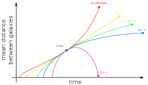
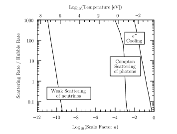
Armed with an understanding of the evolution of the scale factor and the densities of the constituents in the universe, we can extrapolate backwards to explore phenomena at early times. When the universe was much hotter and denser, and the temperature was of order $1 \mathrm{MeV} / k_{\mathrm{B}}$, there were no neutral atoms or even bound nuclei. The vast amounts of highenergy radiation in such a hot environment ensured that any atom or nucleus produced would be immediately destroyed by a high-energy photon. As the universe cooled well below typical nuclear binding energies, light elements began to form in a process known as Big Bang Nucleosynthesis ( $B B N$ ). Knowing the conditions of the early universe and the relevant nuclear cross-sections, we can calculate the expected primordial abundances of all the elements (Ch. 4).
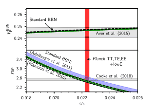
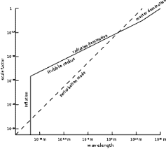
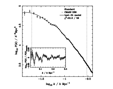
Fig. 1.6 shows the BBN predictions for the abundances of helium and deuterium as a function of the mean baryon density, essentially the density of ordinary matter (Sect. 2.4) in the universe, in units of the critical density. The predicted abundances, in particular that of deuterium, which we will explore in detail in Ch. 4, depend on the density of protons and neutrons at the time of nucleosynthesis. The combined proton plus neutron density is equal to the baryon density since both protons and neutrons have baryon number one and these are the only baryons around at the time.
The horizontal lines in Fig. $1.6$ show the current measurements of the light element abundances. The deuterium abundance is measured in the intergalactic medium at high redshifts by looking for a subtle absorption feature in the spectrum of distant quasars (see Burles and Tytler, 1998; Cooke et al., 2018 and Exercise 1.3). These measurements of the abundances, combined with BBN calculations, give us a way of measuring the baryon density in the universe, constraining ordinary matter to contribute at most $5 \%$ of the critical density (note that the $x$-axis in Fig. $1.6$ is the baryon density divided by the critical density, but multiplied by $h^2 \simeq 0.5$ ). Since the total matter density today is significantly larger than this-as we will see throughout the book-nucleosynthesis provides a compelling argument for matter that is comprised of neither protons or neutrons. This new type of matter has been dubbed dark matter because it apparently does not emit light. One of the central questions in physics now is: “What is the Dark Matter?”
物理代写|宇宙学代写cosmology代考|The cosmic microwave background
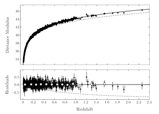
Another phenomenon that falls out of energetics and a qualitative understanding of the evolution of the universe is the origin of the CMB. When the temperature of the radiation was of order $10^4 \mathrm{~K}$ (corresponding to energies of order an $\mathrm{eV}$ ), free electrons and protons combined to form neutral hydrogen. Before then, any hydrogen produced was quickly ionized by energetic photons. After that epoch, at $z \simeq 1100$, the photons that comprise the CMB ceased interacting with any particles and traveled freely through space. When we observe them today, we are thus looking at messengers from an early moment in the universe’s history. They are therefore the most powerful probes of the early universe. We will spend an inordinate amount of time in this book working through the details of what happened to the photons before they last scattered off of free electrons, and also developing the mathematics of the free-streaming process since then. Among many other aspects, we will understand how the CMB constrains the baryon density independently, and in agreement with $\mathrm{BBN}$ as shown in Fig. 1.6, providing a ringing confirmation of the concordance model.
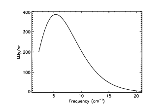
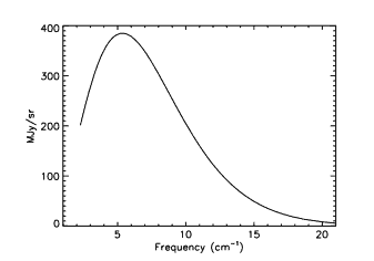
For now, we are only concerned with the crucial fact that the interactions of photons with electrons before last scattering ensured that the photons were in equilibrium. That is, they should have a black-body spectrum. The specific intensity of a gas of photons with a black-body spectrum is
$$
I_v=\frac{4 \pi \hbar v^3 / c^2}{\exp \left[2 \pi \hbar v / k_{\mathrm{R}} T\right]-1} .
$$
Fig. $1.7$ shows the remarkable agreement between this prediction (see Exercise 1.4) of Big Bang cosmology and the observations by the FIRAS instrument aboard the COBE satellite. In fact, the CMB provides the best black-body spectrum ever measured. We have been told ${ }^2$ that detection of the $3 \mathrm{~K}$ background by Penzias and Wilson in the mid-1960s was sufficient evidence to decide the controversy in favor of the Big Bang over the Steady State universe, an alternative scenario without any expansion. Penzias and Wilson, though, measured the radiation at just one wavelength. If even their one-wavelength result was enough to tip the scales, the current data depicted in Fig. $1.7$ should send skeptics from the pages of physics journals to the far reaches of radical internet chat groups.
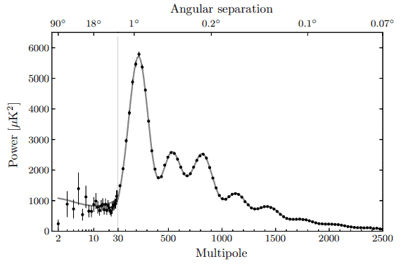
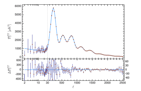
The most important fact we learned from our first 25 years of surveying the CMB was that the early universe was very smooth. No anisotropies were detected in the CMB. This period, while undoubtedly frustrating for observers searching for anisotropies, solidified the view of a smooth Big Bang. The satellite mission COBE discovered anisotropies in the $\mathrm{CMB}$ in 1992, indicating that the early universe was not completely smooth. There were small perturbations in the cosmic plasma, with fractional temperature fluctuations of order $10^{-5}$. By now, these small fluctuations have been mapped with exquisite precision, and the state of the art is to look for even more subtle effects such as CMB polarization and the effect of the intervening matter distribution through gravitational lensing. To understand all of these effects, we must clearly go beyond the smooth background universe and look at deviations from smoothness, or inhomogeneities. Inhomogeneities in the universe are often simply called structure.
宇宙学代考
物理代写|宇宙学代写cosmology代考|大爆炸核合成
有了对尺度因子和宇宙成分密度的演化的理解,我们就可以向后推断,探索早期的现象。当宇宙更热,密度更大,温度为$1 \mathrm{MeV} / k_{\mathrm{B}}$量级时,没有中性原子,甚至连束缚核都没有。在如此高温的环境中,大量的高能辐射保证了产生的任何原子或核都会立即被高能光子摧毁。当宇宙冷却到远低于典型的核结合能时,轻元素开始形成,这个过程被称为大爆炸核合成($B B N$)。知道了早期宇宙的条件和相关的核截面,我们就可以计算出所有元素的预期原始丰度(第4章)
1.6显示了BBN对氦和氘丰度的预测作为平均重子密度的函数,本质上是宇宙中普通物质的密度(第2.4节),以临界密度为单位。预测的丰度,特别是氘的丰度,我们将在第4章中详细探讨,取决于核合成时质子和中子的密度。质子和中子的密度之和等于重子密度,因为质子和中子都有1号重子,而这些是当时周围唯一的重子 图$1.6$中的水平线显示了当前对轻元素丰度的测量。通过在遥远类星体的光谱中寻找细微的吸收特征(见Burles和Tytler, 1998;Cooke等人,2018和练习1.3)。这些丰度的测量,结合BBN的计算,为我们提供了一种测量宇宙重子密度的方法,约束普通物质最多贡献$5 \%$的临界密度(注意,图$1.6$中的$x$轴是重子密度除以临界密度,但乘以$h^2 \simeq 0.5$)。由于现在物质的总密度远远大于这个——正如我们将在全书中看到的那样——核合成为既不是由质子也不是由中子组成的物质提供了一个令人信服的论据。这种新型物质被称为暗物质,因为它显然不发光。现在物理学的核心问题之一是:“暗物质是什么?”
物理代写|宇宙学代写cosmology代考|宇宙微波背景
另一个脱离能量学和对宇宙演化的定性理解的现象是宇宙微波背景辐射的起源。当辐射温度为$10^4 \mathrm{~K}$阶(对应于能量为$\mathrm{eV}$阶)时,自由电子和质子结合形成中性氢。在此之前,任何产生的氢都会被高能光子迅速电离。在那个时代之后,在$z \simeq 1100$处,构成CMB的光子不再与任何粒子相互作用,而是在空间中自由穿行。因此,当我们今天观察它们时,我们看到的是宇宙历史早期的信使。因此,它们是早期宇宙最强大的探测器。在这本书中,我们将花大量的时间研究光子最后一次被自由电子散射之前发生的事情的细节,并从那时起发展自由流过程的数学。在许多其他方面中,我们将了解CMB如何独立地约束重子密度,并与图1.6所示的$\mathrm{BBN}$一致,为一致性模型提供了一个清晰的确认
现在,我们只关心这样一个重要的事实:在最后一次散射之前,光子与电子的相互作用确保了光子处于平衡状态。也就是说,它们应该有一个黑体光谱。具有黑体谱的光子气体的比强度
$$
I_v=\frac{4 \pi \hbar v^3 / c^2}{\exp \left[2 \pi \hbar v / k_{\mathrm{R}} T\right]-1} .
$$
$1.7$显示了大爆炸宇宙学的这一预测(见练习1.4)与COBE卫星上的FIRAS仪器的观测结果之间的显著一致。事实上,CMB提供了迄今为止测量过的最好的黑体光谱。我们被告知${ }^2$,彭齐亚斯和威尔逊在20世纪60年代中期对$3 \mathrm{~K}$背景的探测,足以证明这场争论支持大爆炸而不是稳定状态宇宙,稳定状态宇宙是没有任何膨胀的另一种情况。不过,彭齐亚斯和威尔逊只测量了一种波长的辐射。如果他们的单波长结果就足以扭转这一趋势,那么图$1.7$中所描述的当前数据应该会把怀疑论者从物理期刊的页面送到激进的互联网聊天群中去
我们从最初25年的CMB调查中了解到的最重要的事实是,早期的宇宙是非常平滑的。CMB中未检测到各向异性。这一时期无疑使寻找各向异性的观测者感到沮丧,但却巩固了平稳大爆炸的观点。1992年,COBE卫星任务在$\mathrm{CMB}$中发现了各向异性,这表明早期宇宙并不是完全光滑的。在宇宙等离子体中有微小的扰动,温度波动的分数阶为$10^{-5}$。到目前为止,这些微小的波动已经被精确地绘制出来,而目前的技术水平是寻找更微妙的效应,如CMB偏振和通过引力透镜的干涉物质分布的影响。要理解所有这些效应,我们必须清楚地超越平滑的背景宇宙,并观察平滑的偏差或非均质性。宇宙中的不均匀性通常被简单地称为结构

统计代写请认准statistics-lab™. statistics-lab™为您的留学生涯保驾护航。
金融工程代写
金融工程是使用数学技术来解决金融问题。金融工程使用计算机科学、统计学、经济学和应用数学领域的工具和知识来解决当前的金融问题,以及设计新的和创新的金融产品。
非参数统计代写
非参数统计指的是一种统计方法,其中不假设数据来自于由少数参数决定的规定模型;这种模型的例子包括正态分布模型和线性回归模型。
广义线性模型代考
广义线性模型(GLM)归属统计学领域,是一种应用灵活的线性回归模型。该模型允许因变量的偏差分布有除了正态分布之外的其它分布。
术语 广义线性模型(GLM)通常是指给定连续和/或分类预测因素的连续响应变量的常规线性回归模型。它包括多元线性回归,以及方差分析和方差分析(仅含固定效应)。
有限元方法代写
有限元方法(FEM)是一种流行的方法,用于数值解决工程和数学建模中出现的微分方程。典型的问题领域包括结构分析、传热、流体流动、质量运输和电磁势等传统领域。
有限元是一种通用的数值方法,用于解决两个或三个空间变量的偏微分方程(即一些边界值问题)。为了解决一个问题,有限元将一个大系统细分为更小、更简单的部分,称为有限元。这是通过在空间维度上的特定空间离散化来实现的,它是通过构建对象的网格来实现的:用于求解的数值域,它有有限数量的点。边界值问题的有限元方法表述最终导致一个代数方程组。该方法在域上对未知函数进行逼近。[1] 然后将模拟这些有限元的简单方程组合成一个更大的方程系统,以模拟整个问题。然后,有限元通过变化微积分使相关的误差函数最小化来逼近一个解决方案。
tatistics-lab作为专业的留学生服务机构,多年来已为美国、英国、加拿大、澳洲等留学热门地的学生提供专业的学术服务,包括但不限于Essay代写,Assignment代写,Dissertation代写,Report代写,小组作业代写,Proposal代写,Paper代写,Presentation代写,计算机作业代写,论文修改和润色,网课代做,exam代考等等。写作范围涵盖高中,本科,研究生等海外留学全阶段,辐射金融,经济学,会计学,审计学,管理学等全球99%专业科目。写作团队既有专业英语母语作者,也有海外名校硕博留学生,每位写作老师都拥有过硬的语言能力,专业的学科背景和学术写作经验。我们承诺100%原创,100%专业,100%准时,100%满意。
随机分析代写
随机微积分是数学的一个分支,对随机过程进行操作。它允许为随机过程的积分定义一个关于随机过程的一致的积分理论。这个领域是由日本数学家伊藤清在第二次世界大战期间创建并开始的。
时间序列分析代写
随机过程,是依赖于参数的一组随机变量的全体,参数通常是时间。 随机变量是随机现象的数量表现,其时间序列是一组按照时间发生先后顺序进行排列的数据点序列。通常一组时间序列的时间间隔为一恒定值(如1秒,5分钟,12小时,7天,1年),因此时间序列可以作为离散时间数据进行分析处理。研究时间序列数据的意义在于现实中,往往需要研究某个事物其随时间发展变化的规律。这就需要通过研究该事物过去发展的历史记录,以得到其自身发展的规律。
回归分析代写
多元回归分析渐进(Multiple Regression Analysis Asymptotics)属于计量经济学领域,主要是一种数学上的统计分析方法,可以分析复杂情况下各影响因素的数学关系,在自然科学、社会和经济学等多个领域内应用广泛。
MATLAB代写
MATLAB 是一种用于技术计算的高性能语言。它将计算、可视化和编程集成在一个易于使用的环境中,其中问题和解决方案以熟悉的数学符号表示。典型用途包括:数学和计算算法开发建模、仿真和原型制作数据分析、探索和可视化科学和工程图形应用程序开发,包括图形用户界面构建MATLAB 是一个交互式系统,其基本数据元素是一个不需要维度的数组。这使您可以解决许多技术计算问题,尤其是那些具有矩阵和向量公式的问题,而只需用 C 或 Fortran 等标量非交互式语言编写程序所需的时间的一小部分。MATLAB 名称代表矩阵实验室。MATLAB 最初的编写目的是提供对由 LINPACK 和 EISPACK 项目开发的矩阵软件的轻松访问,这两个项目共同代表了矩阵计算软件的最新技术。MATLAB 经过多年的发展,得到了许多用户的投入。在大学环境中,它是数学、工程和科学入门和高级课程的标准教学工具。在工业领域,MATLAB 是高效研究、开发和分析的首选工具。MATLAB 具有一系列称为工具箱的特定于应用程序的解决方案。对于大多数 MATLAB 用户来说非常重要,工具箱允许您学习和应用专业技术。工具箱是 MATLAB 函数(M 文件)的综合集合,可扩展 MATLAB 环境以解决特定类别的问题。可用工具箱的领域包括信号处理、控制系统、神经网络、模糊逻辑、小波、仿真等。