物理代写|量子场论代写Quantum field theory代考|PHYS3101
如果你也在 怎样代写量子场论Quantum field theory这个学科遇到相关的难题,请随时右上角联系我们的24/7代写客服。
在理论物理学中,量子场论(QFT)是一个理论框架,它结合了经典场论、狭义相对论和量子力学。QFT在粒子物理学中被用来构建亚原子粒子的物理模型,在凝聚态物理学中被用来构建类粒子的模型。
statistics-lab™ 为您的留学生涯保驾护航 在代写量子场论Quantum field theory方面已经树立了自己的口碑, 保证靠谱, 高质且原创的统计Statistics代写服务。我们的专家在代写量子场论Quantum field theory代写方面经验极为丰富,各种代写量子场论Quantum field theory相关的作业也就用不着说。
我们提供的量子场论Quantum field theory及其相关学科的代写,服务范围广, 其中包括但不限于:
- Statistical Inference 统计推断
- Statistical Computing 统计计算
- Advanced Probability Theory 高等概率论
- Advanced Mathematical Statistics 高等数理统计学
- (Generalized) Linear Models 广义线性模型
- Statistical Machine Learning 统计机器学习
- Longitudinal Data Analysis 纵向数据分析
- Foundations of Data Science 数据科学基础
物理代写|量子场论代写Quantum field theory代考|A First Contact with Creation and Annihilation Operators
High-energy interacting particles create other particles, and a relativistic theory must consider multiparticle systems, where the number of particles may vary.
Let us describe what is probably the simplest example of a multiparticle system. ${ }^{67}$ The “particles” are as simple as possible. ${ }^{68}$
Consider a separable Hilbert space with an orthonormal basis $\left(e_{n}\right){n \geq 0}$. The idea is that the state of the system is described by $e{n}$ when the system consists of $n$ particles. The important structure consists of the operators $a$ and $a^{\dagger}$ defined on the domain
$$
\mathcal{D}=\left{\sum_{n \geq 0} \alpha_{n} e_{n} ; \sum_{n \geq 0} n\left|\alpha_{n}\right|^{2}<\infty\right}
$$
by
$$
a\left(e_{n}\right)=\sqrt{n} e_{n-1} ; a^{\dagger}\left(e_{n}\right)=\sqrt{n+1} e_{n+1} .
$$
The definition of $a\left(e_{n}\right)$ is to be understood as $a\left(e_{0}\right)=0$ when $n=0$. The reason for the factors $\sqrt{n}$ and $\sqrt{n+1}$ is not intuitive, and will become clear only gradually.
The notation is consistent, since for each $n, m$,
$$
\left(e_{n}, a\left(e_{m}\right)\right)=\sqrt{m} \delta_{n}^{m-1}=\sqrt{m} \delta_{n+1}^{m}=\left(a^{\dagger}\left(e_{n}\right), e_{m}\right)
$$
where $\delta_{n}^{m}$ is the Kronecker symbol (equal to 1 if $n=m$ and to 0 otherwise).
Exercise 2.17.1 Prove that $a^{\dagger}$ is the adjoint of $a$. Prove in particular that if $|(y, a(x))| \leq$ $C|x|$ for $x \in \mathcal{D}$ then $y \in \mathcal{D}$.
Exercise 2.17.2 Prove that for each $\lambda \in \mathbb{C}$ the operator $a$ has an eigenvector with eigenvalue $\lambda$. Can this happen for a symmetric operator?
It should be obvious from $(2.88)$ that
$$
a^{\dagger} a\left(e_{n}\right)=n e_{n} ; a a^{\dagger}\left(e_{n}\right)=(n+1) e_{n} .
$$
Let us then consider the self-adjoint operator ${ }^{69}$
$$
N:=a^{\dagger} a .
$$
Thus $N\left(e_{n}\right)=n e_{n}$. Since a system in state $e_{n}$ has $n$ particles, the observable corresponding to this operator is “the number of particles”. The operator $N$ is therefore called the number operator.
As another consequence of $(2.90)$,
$$
\left[a, a^{\dagger}\right]\left(e_{n}\right)=e_{n t}
$$
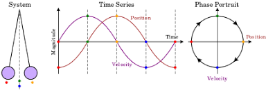
物理代写|量子场论代写Quantum field theory代考|The Harmonic Oscillator
The fundamental structure outlined in the previous section is connected to an equally fundamental system, the harmonic oscillator. A classical one-dimensional harmonic oscillator of angular frequency ${ }^{73} \omega$ consists of a point of mass $m$ on the real line which is pulled back to the origin with a force $m \omega^{2}$ times the distance to the origin. The quantum version of this system is the space $\mathcal{H}=L^{2}(\mathbb{R})$ with Hamiltonian
$$
H:=\frac{1}{2 m}\left(P^{2}+\omega^{2} m^{2} X^{2}\right),
$$
where $P$ and $X$ are respectively the momentum and the position operators of Section $2.5$. This is the Hamiltonian $(2.79)$ in the case where $V(x)=m \omega^{2} x^{2} / 2$. That this formula provides a quantized version of the classical harmonic oscillator is not obvious at all. ${ }^{74}$ We will explain in Section $6.6$ the systematic procedure of “canonical quantization” to discover formulas such as (2.77) or (2.95). This procedure is by no means a proof of anything, and the resulting formulas are justified only by the fact that they provide a fruitful model. So there is little harm to accept at this stage that the formula (2.95) is indeed fundamental. We have not proved yet that this formula defines a self-adjoint operator, but this is a consequence of the analysis below.
Exercise 2.18.1 Prove that a symmetric operator which admits an orthonormal basis of eigenvectors is self-adjoint. Hint: If we denote by $\left(e_{n}\right)$ an orthonormal basis of eigenvectors, and $\lambda_{n}$ the eigenvalue of $e_{n}$, the natural domain $\mathcal{D}$ of the operator is
$$
\left{x=\sum_{n} x_{n} e_{n} ; \sum_{n}\left(1+\left|\lambda_{n}\right|^{2}\right)\left|x_{n}\right|^{2}<\infty\right}
$$
The program for this section is first to find a basis of eigenvectors for the Hamiltonian (2.95), and then to examine how some classical quantities transform under quantization.
物理代写|量子场论代写Quantum field theory代考|Tensor Products
The present section is standard material, but our presentation attempts to balance rigor and readability.
Principle 6 If the states of two systems $\mathcal{S}{1}$ and $\mathcal{S}{2}$ are represented by the unitary rays in two Hilbert spaces $\mathcal{H}{1}$ and $\mathcal{H}{2}$ respectively, the appropriate Hilbert space to represent the system consisting of the union of $\mathcal{S}{1}$ and $\mathcal{S}{2}$ is the tensor product $\mathcal{H}{1} \otimes \mathcal{H}{2}$.
Our first task is to describe this space. ${ }^{2}$ A mathematician would love to see an “intrinsic” definition of this tensor product, a definition that does not use bases or a special representation of these Hilbert spaces. This can be done elegantly as in e.g. Dimock’s book [23]. We shall not enjoy this piece of abstraction and we shall go the ugly way.
If $\left(e_{n}\right){n \geq 1}$ is an orthonormal basis of $\mathcal{H}{1}$ and $\left(f_{n}\right){n \geq 1}$ is an orthonormal basis of $\mathcal{H}{2}$ then the vectors $e_{n} \otimes f_{m}$ constitute an orthonormal basis of $\mathcal{H}{1} \otimes \mathcal{H}{2}$, which is thus the set of vectors of the type $\sum_{n, m \geq 1} a_{n, m} e_{n} \otimes f_{m}$ where the complex numbers $a_{n, m}$ satisfy $\sum_{n, m \geq 1}\left|a_{n, m}\right|^{2}<\infty$. Here the quantity $e_{n} \otimes f_{m}$ is just a notation, which is motivated by the fact that for $x=\sum_{n \geq 1} \alpha_{n} e_{n} \in \mathcal{H}{1}$ and $y=\sum{n \geq 1} \beta_{n} f_{n} \in \mathcal{H}{2}$ one defines $x \otimes y \in$ $\mathcal{H}{1} \otimes \mathcal{H}{2}$ by $$ x \otimes y=\sum{m, n \geq 1} \alpha_{n} \beta_{m} e_{n} \otimes f_{m} .
$$
When either $\mathcal{H}{1}$ or $\mathcal{H}{2}$, or both, are finite-dimensional, the definition is modified in the obvious manner.
Exercise 3.1.1 When $\mathcal{H}{1}$ and $\mathcal{H}{2}$ are finite-dimensional, what is the dimension of $\mathcal{H}{1} \otimes \mathcal{H}{2}$ ? How does it compare with the dimension of the usual product $\mathcal{H}{1} \times \mathcal{H}{2}$ ?
When either $\mathcal{H}{1}$ or $\mathcal{H}{2}$ is infinite-dimensional, $\mathcal{H}{1} \otimes \mathcal{H}{2}$ is an infinite-dimensional Hilbert space. The important structure is the bilinear form from $\mathcal{H}{1} \times \mathcal{H}{2}$ into this space given by (3.1).
Recalling that $(x, y)$ denotes the inner product in a Hilbert space we observe the formula
$$
\left(x \otimes y, x^{\prime} \otimes y^{\prime}\right)=\left(x, x^{\prime}\right)\left(y, y^{\prime}\right),
$$
which is a straightforward consequence of the fact that the basis $e_{n} \otimes f_{m}$ is orthonormal. $^{3}$
The problem with our definition of the tensor product is that one is supposed to check that “it does not depend on the choice of the orthonormal basis”, a tedious task that joins similar tasks under the carpet. ${ }^{4}$ The good news is that all the identifications one may wish for are true. If both $\mathcal{H}{1}$ and $\mathcal{H}{2}$ are the space of square-integrable functions on $\mathbb{R}^{3}$, then $\mathcal{H}{1} \otimes \mathcal{H}{2}$ is the space of square-integrable functions on $\mathbb{R}^{6} .5$ This fits very well with the Dirac formalism: If $|x\rangle$ denotes the Dirac function at $\boldsymbol{x}$, (so that these generalized vectors provide a generalized basis of $\mathcal{H}{1}$, and similarly for $|\boldsymbol{y}\rangle$, then $|\boldsymbol{x}\rangle|\boldsymbol{y}\rangle$ denotes the Dirac function at the point $(\boldsymbol{x}, \boldsymbol{y}) \in \mathbb{R}^{6}$, and these generalized vectors provide a generalized basis of $\mathcal{H}{1} \otimes \mathcal{H}{2}$. Furthermore, if $f \in \mathcal{H}{1}$ and $g \in \mathcal{H}_{2}$ then $f \otimes g$ identifies with the function $(\boldsymbol{x}, \boldsymbol{y}) \mapsto$ $f(x) g(y)$ on $\mathbb{R}^{6}$.
量子场论代考
物理代写|量子场论代写Quantum field theory代考|A First Contact with Creation and Annihilation Operators
高能相互作用的粒子会产生其他粒子,相对论必须考虑多粒子系统,其中粒子的数量可能会有所不同。
让我们描述一下可能是多粒子系统最简单的例子。67“粒子”尽可能简单。68
考虑具有标准正交基的可分离希尔伯特空间(和n)n≥0. 这个想法是系统的状态描述为和n当系统由n粒子。重要结构由运算符组成一个和一个†在域上定义
\mathcal{D}=\left{\sum_{n \geq 0} \alpha_{n}e_{n} ; \sum_{n \geq 0} n\left|\alpha_{n}\right|^{2}<\infty\right}\mathcal{D}=\left{\sum_{n \geq 0} \alpha_{n}e_{n} ; \sum_{n \geq 0} n\left|\alpha_{n}\right|^{2}<\infty\right}
经过
一个(和n)=n和n−1;一个†(和n)=n+1和n+1.
的定义一个(和n)应理解为一个(和0)=0什么时候n=0. 因素的原因n和n+1不直观,只会逐渐清晰。
符号是一致的,因为对于每个n,米,
(和n,一个(和米))=米dn米−1=米dn+1米=(一个†(和n),和米)
在哪里dn米是克罗内克符号(如果n=米否则为 0)。
练习 2.17.1 证明一个†是的伴随一个. 特别证明如果|(是,一个(X))|≤ C|X|为了X∈D然后是∈D.
练习 2.17.2 证明对于每个λ∈C运营商一个有一个带有特征值的特征向量λ. 对称算子会发生这种情况吗?
应该是显而易见的(2.88)那
一个†一个(和n)=n和n;一个一个†(和n)=(n+1)和n.
然后让我们考虑自伴算子69
ñ:=一个†一个.
因此ñ(和n)=n和n. 由于系统处于状态和n有n粒子,这个算子对应的 observable 就是“粒子个数”。运营商ñ因此称为数运算符。
作为另一个结果(2.90),
[一个,一个†](和n)=和n吨
物理代写|量子场论代写Quantum field theory代考|The Harmonic Oscillator
上一节中概述的基本结构连接到一个同样基本的系统,即谐振子。一种经典的角频率一维谐振子73ω由一个质点组成米在用力拉回原点的实线上米ω2乘以到原点的距离。这个系统的量子版本是空间H=大号2(R)与哈密顿量
H:=12米(磷2+ω2米2X2),
在哪里磷和X分别是截面的动量算子和位置算子2.5. 这是哈密顿量(2.79)在这种情况下在(X)=米ω2X2/2. 这个公式提供了经典谐振子的量化版本,这一点并不明显。74我们将在章节中解释6.6“规范量化”的系统过程以发现诸如 (2.77) 或 (2.95) 之类的公式。这个过程绝不是任何事情的证明,并且得到的公式仅通过它们提供了一个富有成效的模型这一事实来证明是合理的。因此,在这个阶段接受公式(2.95)确实是基本的并没有什么坏处。我们还没有证明这个公式定义了一个自伴算子,但这是下面分析的结果。
练习 2.18.1 证明一个对称算子承认特征向量的正交基是自伴的。提示:如果我们用(和n)特征向量的正交基,和λn的特征值和n, 自然域D运营商是
\left{x=\sum_{n} x_{n} e_{n} ; \sum_{n}\left(1+\left|\lambda_{n}\right|^{2}\right)\left|x_{n}\right|^{2}<\infty\right}\left{x=\sum_{n} x_{n} e_{n} ; \sum_{n}\left(1+\left|\lambda_{n}\right|^{2}\right)\left|x_{n}\right|^{2}<\infty\right}
本节的程序是首先找到哈密顿量(2.95)的特征向量的基,然后检查一些经典量在量化下是如何变换的。
物理代写|量子场论代写Quantum field theory代考|Tensor Products
本节是标准材料,但我们的演示文稿试图平衡严谨性和可读性。
原则 6 如果两个系统的状态小号1和小号2由两个希尔伯特空间中的酉射线表示H1和H2分别地,适当的希尔伯特空间来表示由联合组成的系统小号1和小号2是张量积H1⊗H2.
我们的首要任务是描述这个空间。2数学家很想看到这个张量积的“内在”定义,一个不使用基的定义或这些希尔伯特空间的特殊表示。这可以优雅地完成,例如 Dimock 的书 [23]。我们不会享受这种抽象,我们会走上丑陋的道路。
如果(和n)n≥1是一个正交基H1和(Fn)n≥1是一个正交基H2然后向量和n⊗F米构成一个正交基H1⊗H2,因此是该类型的向量集∑n,米≥1一个n,米和n⊗F米其中复数一个n,米满足∑n,米≥1|一个n,米|2<∞. 这里的数量和n⊗F米只是一个符号,其动机是因为X=∑n≥1一个n和n∈H1和是=∑n≥1bnFn∈H2一个定义X⊗是∈ H1⊗H2经过
X⊗是=∑米,n≥1一个nb米和n⊗F米.
当H1或者H2,或两者都是有限维的,定义以明显的方式修改。
练习 3.1.1 何时H1和H2是有限维的,什么是维H1⊗H2? 它与通常产品的尺寸相比如何H1×H2?
当H1或者H2是无限维的,H1⊗H2是无限维希尔伯特空间。重要的结构是来自的双线性形式H1×H2进入由(3.1)给出的这个空间。
回想起来(X,是)表示希尔伯特空间中的内积,我们观察公式
(X⊗是,X′⊗是′)=(X,X′)(是,是′),
这是一个直接的结果,即基础和n⊗F米是正交的。3
我们对张量积的定义存在的问题是,我们应该检查“它不依赖于正交基的选择”,这是一项繁琐的任务,需要在地毯下加入类似的任务。4好消息是,人们可能希望得到的所有身份都是真实的。如果两者H1和H2是平方可积函数的空间R3, 然后H1⊗H2是平方可积函数的空间R6.5这非常符合狄拉克的形式主义:如果|X⟩表示狄拉克函数X, (因此这些广义向量提供了H1, 同样对于|是⟩, 然后|X⟩|是⟩表示该点的狄拉克函数(X,是)∈R6, 这些广义向量提供了一个广义基础H1⊗H2. 此外,如果F∈H1和G∈H2然后F⊗G与功能标识(X,是)↦ F(X)G(是)上R6.

统计代写请认准statistics-lab™. statistics-lab™为您的留学生涯保驾护航。
金融工程代写
金融工程是使用数学技术来解决金融问题。金融工程使用计算机科学、统计学、经济学和应用数学领域的工具和知识来解决当前的金融问题,以及设计新的和创新的金融产品。
非参数统计代写
非参数统计指的是一种统计方法,其中不假设数据来自于由少数参数决定的规定模型;这种模型的例子包括正态分布模型和线性回归模型。
广义线性模型代考
广义线性模型(GLM)归属统计学领域,是一种应用灵活的线性回归模型。该模型允许因变量的偏差分布有除了正态分布之外的其它分布。
术语 广义线性模型(GLM)通常是指给定连续和/或分类预测因素的连续响应变量的常规线性回归模型。它包括多元线性回归,以及方差分析和方差分析(仅含固定效应)。
有限元方法代写
有限元方法(FEM)是一种流行的方法,用于数值解决工程和数学建模中出现的微分方程。典型的问题领域包括结构分析、传热、流体流动、质量运输和电磁势等传统领域。
有限元是一种通用的数值方法,用于解决两个或三个空间变量的偏微分方程(即一些边界值问题)。为了解决一个问题,有限元将一个大系统细分为更小、更简单的部分,称为有限元。这是通过在空间维度上的特定空间离散化来实现的,它是通过构建对象的网格来实现的:用于求解的数值域,它有有限数量的点。边界值问题的有限元方法表述最终导致一个代数方程组。该方法在域上对未知函数进行逼近。[1] 然后将模拟这些有限元的简单方程组合成一个更大的方程系统,以模拟整个问题。然后,有限元通过变化微积分使相关的误差函数最小化来逼近一个解决方案。
tatistics-lab作为专业的留学生服务机构,多年来已为美国、英国、加拿大、澳洲等留学热门地的学生提供专业的学术服务,包括但不限于Essay代写,Assignment代写,Dissertation代写,Report代写,小组作业代写,Proposal代写,Paper代写,Presentation代写,计算机作业代写,论文修改和润色,网课代做,exam代考等等。写作范围涵盖高中,本科,研究生等海外留学全阶段,辐射金融,经济学,会计学,审计学,管理学等全球99%专业科目。写作团队既有专业英语母语作者,也有海外名校硕博留学生,每位写作老师都拥有过硬的语言能力,专业的学科背景和学术写作经验。我们承诺100%原创,100%专业,100%准时,100%满意。
随机分析代写
随机微积分是数学的一个分支,对随机过程进行操作。它允许为随机过程的积分定义一个关于随机过程的一致的积分理论。这个领域是由日本数学家伊藤清在第二次世界大战期间创建并开始的。
时间序列分析代写
随机过程,是依赖于参数的一组随机变量的全体,参数通常是时间。 随机变量是随机现象的数量表现,其时间序列是一组按照时间发生先后顺序进行排列的数据点序列。通常一组时间序列的时间间隔为一恒定值(如1秒,5分钟,12小时,7天,1年),因此时间序列可以作为离散时间数据进行分析处理。研究时间序列数据的意义在于现实中,往往需要研究某个事物其随时间发展变化的规律。这就需要通过研究该事物过去发展的历史记录,以得到其自身发展的规律。
回归分析代写
多元回归分析渐进(Multiple Regression Analysis Asymptotics)属于计量经济学领域,主要是一种数学上的统计分析方法,可以分析复杂情况下各影响因素的数学关系,在自然科学、社会和经济学等多个领域内应用广泛。
MATLAB代写
MATLAB 是一种用于技术计算的高性能语言。它将计算、可视化和编程集成在一个易于使用的环境中,其中问题和解决方案以熟悉的数学符号表示。典型用途包括:数学和计算算法开发建模、仿真和原型制作数据分析、探索和可视化科学和工程图形应用程序开发,包括图形用户界面构建MATLAB 是一个交互式系统,其基本数据元素是一个不需要维度的数组。这使您可以解决许多技术计算问题,尤其是那些具有矩阵和向量公式的问题,而只需用 C 或 Fortran 等标量非交互式语言编写程序所需的时间的一小部分。MATLAB 名称代表矩阵实验室。MATLAB 最初的编写目的是提供对由 LINPACK 和 EISPACK 项目开发的矩阵软件的轻松访问,这两个项目共同代表了矩阵计算软件的最新技术。MATLAB 经过多年的发展,得到了许多用户的投入。在大学环境中,它是数学、工程和科学入门和高级课程的标准教学工具。在工业领域,MATLAB 是高效研究、开发和分析的首选工具。MATLAB 具有一系列称为工具箱的特定于应用程序的解决方案。对于大多数 MATLAB 用户来说非常重要,工具箱允许您学习和应用专业技术。工具箱是 MATLAB 函数(M 文件)的综合集合,可扩展 MATLAB 环境以解决特定类别的问题。可用工具箱的领域包括信号处理、控制系统、神经网络、模糊逻辑、小波、仿真等。