如果你也在 怎样代写多元统计分析Multivariate Statistical Analysis这个学科遇到相关的难题，请随时右上角联系我们的24/7代写客服。

多变量统计分析被认为是评估地球化学异常与任何单独变量和变量之间相互影响的意义的有用工具。

statistics-lab™ 为您的留学生涯保驾护航 在代写多元统计分析Multivariate Statistical Analysis方面已经树立了自己的口碑, 保证靠谱, 高质且原创的统计Statistics代写服务。我们的专家在代写多元统计分析Multivariate Statistical Analysis代写方面经验极为丰富，各种代写多元统计分析Multivariate Statistical Analysis相关的作业也就用不着说。

我们提供的多元统计分析Multivariate Statistical Analysis及其相关学科的代写，服务范围广, 其中包括但不限于:

• Statistical Inference 统计推断
• Statistical Computing 统计计算
• Advanced Probability Theory 高等概率论
• Advanced Mathematical Statistics 高等数理统计学
• (Generalized) Linear Models 广义线性模型
• Statistical Machine Learning 统计机器学习
• Longitudinal Data Analysis 纵向数据分析
• Foundations of Data Science 数据科学基础

统计代写|多元统计分析代写Multivariate Statistical Analysis代考|Scatterplots

Scatterplots are bivariate or trivariate plots of variables against each other. They help us understand relationships among the variables of a data set. A downward-sloping scatter indicates that as we increase the variable on the horizontal axis, the variable on the vertical axis decreases. An analogous statement can be made for upward-sloping scatters.

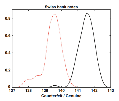
Figure $1.12$ plots the fifth column (upper inner frame) of the bank data against the sixth column (diagonal). The scatter is downward-sloping. As we already know from the previous section on marginal comparison (e.g., Fig. 1.9) a good separation between genuine and counterfeit banknotes is visible for the diagonal variable. The sub-cloud in the upper half (circles) of Fig. $1.12$ corresponds to the true banknotes. As noted before, this separation is not distinct, since the two groups overlap somewhat.
This can be verified in an interactive computing environment by showing the index and coordinates of certain points in this scatterplot. In Fig. 1.12, the 70th observation in the merged data set is given as a thick circle, and it is from a genuine bank note. This observation lies well embedded in the cloud of counterfeit banknotes. One straightforward approach that could be used to tell the counterfeit from the genuine banknotes is to draw a straight line and define notes above this value as genuine. We would, of course, misclassify the 70th observation, but can we do better?

If we extend the two-dimensional scatterplot by adding a third variable, e.g., $X_4$ (lower distance to inner frame), we obtain the scatterplot in three dimensions as shown in Fig. 1.13. It becomes apparent from the location of the point clouds that a better separation is obtained. We have rotated the three-dimensional data until this satisfactory 3D view was obtained. Later, we will see that the rotation is the same as bunding a high-dimensional observation into one or more linear combinations of the elements of the observation vector. In other words, the “separation line” parallel to the horizontal coordinate axis in Fig. $1.12$ is, in Fig. 1.13, a plane and no longer parallel to one of the axes. The formula for such a separation plane is a linear combination of the elements of the observation vector:
$$
a_1 x_1+a_2 x_2+\cdots+a_6 x_6=\text { const. }
$$
The algorithm that automatically finds the weights $\left(a_1, \ldots, a_6\right)$ will be investigated later on in Chap. 14.

Let us study yet another technique: the scatterplot matrix. If we want to draw all possible two-dimensional scatterplots for the variables, we can create a so-called draftsman’s plot (named after a draftsman who prepares drafts for parliamentary discussions). Similar to a draftsman’s plot the scatterplot matrix helps in creating new ideas and in building knowledge about dependencies and structure.

统计代写|多元统计分析代写Multivariate Statistical Analysis代考|Chernoff-Flury Faces

If we are given a data in a numerical form, we tend to also display it numerically. This was done in the preceding sections: an observation $x_1=(1,2)$ was plotted as the point $(1,2)$ in a two-dimensional coordinate system. In multivariate analysis, we want to understand data in low dimensions (e.g., on a $2 \mathrm{D}$ computer screen) although the structures are hidden in high dimensions. The numerical display of data structures using coordinates, therefore, ends at dimensions greater than three.

If we are interested in condensing a structure into 2 D elements, we have to consider alternative graphical techniques. The Chernoff-Flury faces, for example, provide such a condensation of high-dimensional information into a simple “face”. In fact, faces are a simple way of graphically displaying high-dimensional data. The size of the face elements like pupils, eyes, upper and lower hair line, etc., are assigned to certain variables. The idea of using faces goes back to Chernoff (1973) and has been further developed by Bernhard Flury. We follow the design described in Flury and Riedwyl (1988) which uses the following characteristics:

First, every variable that is to be coded into a characteristic face element is transformed into a $(0,1)$ scale, i.e., the minimum of the variable corresponds to 0 and the maximum to 1 . The extreme positions of the face elements, therefore, correspond to a certain “grin” or “happy” face element. Dark hair might be coded as 1, and blond hair as 0 and so on.

As an example, consider the observations 91 to 110 of the bank data. Recall that the bank data set consists of 200 observations of dimension 6 where, for example, $X_6$ is the diagonal of the note. If we assign the six variables to the following face elements:
$$
\begin{aligned}
& X_1=1,19 \text { (eye sizes) } \
& X_2=2,20 \text { (pupil sizes) } \
& X_3=4,22 \text { (eye slants) } \
& X_4=11,29 \text { (upper hair lines) } \
& X_5=12,30 \text { (lower hair lines) } \
& X_6=13,14,31,32 \text { (face lines and darkness of hair), }
\end{aligned}
$$
we obtain Fig. 1.15.
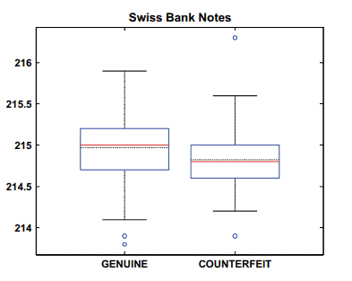
Also recall that observations 1-100 correspond to the genuine notes, and that observations 101-200 correspond to the counterfeit notes. The counterfeit banknotes then correspond to the upper half of Fig. 1.15. In fact, the faces for these observations look more grim and less happy. The variable $X_6$ (diagonal) already worked well in the boxplot on Fig. 1.4 in distinguishing between the counterfeit and genuine notes. Here, this variable is assigned to the face line and the darkness of the hair. That is why we clearly see a good separation within these 20 observations.

What happens if we include all 100 genuine and all 100 counterfeit banknotes in the Chernoff-Flury face technique? Figure $1.16$ shows the faces of the genuine banknotes with the same assignments as used before and Fig. 1.17 shows the faces of the counterfeit banknotes. Comparing Figs. $1.16$ and $1.17$ one clearly sees that the diagonal (face line) is longer for genuine banknotes. Equivalently coded is the hair darkness (diagonal) which is lighter (shorter) for the counterfeit banknotes. One sees that the faces of the genuine banknotes have a much darker appearance and have broader face lines. The faces in Fig. $1.16$ are obviously different from the ones in Fig. 1.17.

多元统计分析代考

统计代写|多元统计分析代写Multivariate Statistical Analysis代考|Scatterplots

散点图是变量相互之间的双变量或三变量图。它们帮助我们理解数据集变量之间的关系。向下倾斜的散点表示随着我们增加水平轴上的变量，垂直轴上的变量减少。对于向上倾斜的散点可以做出类似的陈述。

数字1.12根据第六列（对角线）绘制银行数据的第五列（上部内框）。散点是向下倾斜的。正如我们从前面关于边际比较的部分（例如图 1.9）中已经知道的那样，对角线变量可以很好地区分真钞和假钞。图上半部分（圆圈）的子云。1.12对应真钞。如前所述，这种分离并不明显，因为这两个组有些重叠。
这可以在交互式计算环境中通过显示此散点图中某些点的索引和坐标来验证。在图 1.12 中，合并数据集中的第 70 个观察值以粗圆圈给出，它来自真钞。这一观察结果很好地嵌入了假钞云中。一种可用于区分伪钞和真钞的直接方法是画一条直线并将高于此值的钞票定义为真钞。当然，我们会对第 70 个观察结果进行错误分类，但我们能做得更好吗？

如果我们通过添加第三个变量来扩展二维散点图，例如，X4（到内框的距离更近），我们得到了三个维度的散点图，如图 1.13 所示。从点云的位置可以明显看出获得了更好的分离。我们旋转了三维数据，直到获得令人满意的 3D 视图。稍后，我们将看到旋转与将高维观测值捆绑为观测向量元素的一个或多个线性组合相同。换句话说，平行于图1中横坐标轴的“分离线”。1.12在图 1.13 中是一个平面，不再平行于其中一个轴。这种分离平面的公式是观察向量元素的线性组合：

一个1X1+一个2X2+⋯+一个6X6= 常量。 
自动找到权重的算法(一个1,…,一个6)将在稍后的章节中进行调查。14.

让我们研究另一种技术：散点图矩阵。如果我们想为变量绘制所有可能的二维散点图，我们可以创建一个所谓的绘图员图（以为议会讨论准备草案的绘图员命名）。类似于制图员的绘图，散点图矩阵有助于创造新想法以及建立有关依赖性和结构的知识。

统计代写|多元统计分析代写Multivariate Statistical Analysis代考|Chernoff-Flury Faces

如果给我们一个数字形式的数据，我们也倾向于以数字形式显示它。这是在前面的部分中完成的：观察X1=(1,2)被绘制为点(1,2)在二维坐标系中。在多变量分析中，我们希望了解低维数据（例如，在2丁电脑屏幕）虽然结构隐藏在高维度中。因此，使用坐标的数据结构的数字显示以大于三的维度结束。

如果我们有兴趣将结构压缩成二维元素，我们必须考虑替代图形技术。例如，Chernoff-Flury 面孔将高维信息浓缩到一张简单的“面孔”中。事实上，人脸是一种以图形方式显示高维数据的简单方式。瞳孔、眼睛、上下发际线等面部元素的大小被分配给某些变量。使用面孔的想法可以追溯到 Chernoff (1973)，并由 Bernhard Flury 进一步发展。我们遵循 Flury 和 Riedwyl (1988) 中描述的设计，该设计使用以下特征：

首先，将要编码为特征人脸元素的每个变量转换为(0,1)scale，即变量的最小值对应于 0 ，最大值对应于 1 。因此，面部元素的极端位置对应于某个“咧嘴笑”或“快乐”的面部元素。深色头发可能编码为 1，金色头发编码为 0，依此类推。

例如，考虑银行数据的观察值 91 到 110。回想一下，银行数据集由 200 个维度 6 的观察值组成，例如，X6是音符的对角线。如果我们将六个变量分配给以下面元素：

X1=1,19 （眼睛大小）  X2=2,20 （瞳孔大小）  X3=4,22 （眼睛倾斜）  X4=11,29 （上发际线）  X5=12,30 （下发际线）  X6=13,14,31,32 （面部线条和头发的深色）， 
我们得到图 1.15。
还记得观察值 1-100 对应于真钞，观察值 101-200 对应于假币。伪钞对应于图 1.15 的上半部分。事实上，这些观察结果的面孔看起来更冷酷，更不快乐。变量X6（对角线）在图 1.4 的箱线图中已经很好地区分了假钞和真钞。在这里，这个变量被分配给面部线条和头发的黑度。这就是为什么我们在这 20 个观察结果中清楚地看到了很好的分离。

如果我们将所有 100 张真钞和所有 100 张假钞都包含在 Chernoff-Flury 面部技术中，会发生什么情况？数字1.16图 1.17 显示了具有与之前使用的相同分配的真钞的面，图 1.17 显示了伪钞的面。比较无花果。1.16和1.17可以清楚地看到，真钞的对角线（面线）更长。等效编码是假钞的发色（对角线）较浅（较短）。可以看到，真钞的正面颜色更深，线条更宽。图中的人脸。1.16与图 1.17 中的明显不同。

统计代写请认准statistics-lab™. statistics-lab™为您的留学生涯保驾护航。

金融工程代写

金融工程是使用数学技术来解决金融问题。金融工程使用计算机科学、统计学、经济学和应用数学领域的工具和知识来解决当前的金融问题，以及设计新的和创新的金融产品。

非参数统计代写

非参数统计指的是一种统计方法，其中不假设数据来自于由少数参数决定的规定模型；这种模型的例子包括正态分布模型和线性回归模型。

广义线性模型代考

广义线性模型（GLM）归属统计学领域，是一种应用灵活的线性回归模型。该模型允许因变量的偏差分布有除了正态分布之外的其它分布。

术语 广义线性模型（GLM）通常是指给定连续和/或分类预测因素的连续响应变量的常规线性回归模型。它包括多元线性回归，以及方差分析和方差分析（仅含固定效应）。

有限元方法代写

有限元方法（FEM）是一种流行的方法，用于数值解决工程和数学建模中出现的微分方程。典型的问题领域包括结构分析、传热、流体流动、质量运输和电磁势等传统领域。

有限元是一种通用的数值方法，用于解决两个或三个空间变量的偏微分方程（即一些边界值问题）。为了解决一个问题，有限元将一个大系统细分为更小、更简单的部分，称为有限元。这是通过在空间维度上的特定空间离散化来实现的，它是通过构建对象的网格来实现的：用于求解的数值域，它有有限数量的点。边界值问题的有限元方法表述最终导致一个代数方程组。该方法在域上对未知函数进行逼近。[1] 然后将模拟这些有限元的简单方程组合成一个更大的方程系统，以模拟整个问题。然后，有限元通过变化微积分使相关的误差函数最小化来逼近一个解决方案。

tatistics-lab作为专业的留学生服务机构，多年来已为美国、英国、加拿大、澳洲等留学热门地的学生提供专业的学术服务，包括但不限于Essay代写，Assignment代写，Dissertation代写，Report代写，小组作业代写，Proposal代写，Paper代写，Presentation代写，计算机作业代写，论文修改和润色，网课代做，exam代考等等。写作范围涵盖高中，本科，研究生等海外留学全阶段，辐射金融，经济学，会计学，审计学，管理学等全球99%专业科目。写作团队既有专业英语母语作者，也有海外名校硕博留学生，每位写作老师都拥有过硬的语言能力，专业的学科背景和学术写作经验。我们承诺100%原创，100%专业，100%准时，100%满意。

随机分析代写

随机微积分是数学的一个分支，对随机过程进行操作。它允许为随机过程的积分定义一个关于随机过程的一致的积分理论。这个领域是由日本数学家伊藤清在第二次世界大战期间创建并开始的。

时间序列分析代写

随机过程，是依赖于参数的一组随机变量的全体，参数通常是时间。 随机变量是随机现象的数量表现，其时间序列是一组按照时间发生先后顺序进行排列的数据点序列。通常一组时间序列的时间间隔为一恒定值（如1秒，5分钟，12小时，7天，1年），因此时间序列可以作为离散时间数据进行分析处理。研究时间序列数据的意义在于现实中，往往需要研究某个事物其随时间发展变化的规律。这就需要通过研究该事物过去发展的历史记录，以得到其自身发展的规律。

回归分析代写

多元回归分析渐进（Multiple Regression Analysis Asymptotics）属于计量经济学领域，主要是一种数学上的统计分析方法，可以分析复杂情况下各影响因素的数学关系，在自然科学、社会和经济学等多个领域内应用广泛。

MATLAB代写

MATLAB 是一种用于技术计算的高性能语言。它将计算、可视化和编程集成在一个易于使用的环境中，其中问题和解决方案以熟悉的数学符号表示。典型用途包括：数学和计算算法开发建模、仿真和原型制作数据分析、探索和可视化科学和工程图形应用程序开发，包括图形用户界面构建MATLAB 是一个交互式系统，其基本数据元素是一个不需要维度的数组。这使您可以解决许多技术计算问题，尤其是那些具有矩阵和向量公式的问题，而只需用 C 或 Fortran 等标量非交互式语言编写程序所需的时间的一小部分。MATLAB 名称代表矩阵实验室。MATLAB 最初的编写目的是提供对由 LINPACK 和 EISPACK 项目开发的矩阵软件的轻松访问，这两个项目共同代表了矩阵计算软件的最新技术。MATLAB 经过多年的发展，得到了许多用户的投入。在大学环境中，它是数学、工程和科学入门和高级课程的标准教学工具。在工业领域，MATLAB 是高效研究、开发和分析的首选工具。MATLAB 具有一系列称为工具箱的特定于应用程序的解决方案。对于大多数 MATLAB 用户来说非常重要，工具箱允许您学习和应用专业技术。工具箱是 MATLAB 函数（M 文件）的综合集合，可扩展 MATLAB 环境以解决特定类别的问题。可用工具箱的领域包括信号处理、控制系统、神经网络、模糊逻辑、小波、仿真等。

R语言代写	问卷设计与分析代写
PYTHON代写	回归分析与线性模型代写
MATLAB代写	方差分析与试验设计代写
STATA代写	机器学习/统计学习代写
SPSS代写	计量经济学代写
EVIEWS代写	时间序列分析代写
EXCEL代写	深度学习代写
SQL代写	各种数据建模与可视化代写

如果你也在 怎样代写多元统计分析Multivariate Statistical Analysis这个学科遇到相关的难题，请随时右上角联系我们的24/7代写客服。

多变量统计分析被认为是评估地球化学异常与任何单独变量和变量之间相互影响的意义的有用工具。

statistics-lab™ 为您的留学生涯保驾护航 在代写多元统计分析Multivariate Statistical Analysis方面已经树立了自己的口碑, 保证靠谱, 高质且原创的统计Statistics代写服务。我们的专家在代写多元统计分析Multivariate Statistical Analysis代写方面经验极为丰富，各种代写多元统计分析Multivariate Statistical Analysis相关的作业也就用不着说。

我们提供的多元统计分析Multivariate Statistical Analysis及其相关学科的代写，服务范围广, 其中包括但不限于:

• Statistical Inference 统计推断
• Statistical Computing 统计计算
• Advanced Probability Theory 高等概率论
• Advanced Mathematical Statistics 高等数理统计学
• (Generalized) Linear Models 广义线性模型
• Statistical Machine Learning 统计机器学习
• Longitudinal Data Analysis 纵向数据分析
• Foundations of Data Science 数据科学基础

统计代写|多元统计分析代写Multivariate Statistical Analysis代考|Histograms

Histograms are density estimates. A density estimate gives a good impression of the distribution of the data. In contrast to boxplots, density estimates show possible multimodality of the data. The idea is to locally represent the data density by counting the number of observations in a sequence of consecutive intervals (bins) with origin $x_0$. Let $B_j\left(x_0, h\right)$ denote the bin of length $h$, which is the element of a bin grid starting at $x_0$ :
$$
B_j\left(x_0, h\right)=\left[x_0+(j-1) h, x_0+j h\right), \quad j \in \mathbb{Z},
$$
where $[.,$.$) denotes a left-closed and right-open interval. If \left{x_i\right}_{i=1}^n$ is an i.i.d. sample with density $f$, the histogram is defined as follows:
$$
\widehat{f}h(x)=n^{-1} h^{-1} \sum{j \in \mathbb{Z}} \sum_{i=1}^n \mathrm{I}\left{x_i \in B_j\left(x_0, h\right)\right} \mathrm{I}\left{x \in B_j\left(x_0, h\right)\right} .
$$
In sum (1.7) the first indicator function $\mathrm{I}\left{x_i \in B_j\left(x_0, h\right)\right}$ counts the number of observations falling into bin $B_j\left(x_0, h\right)$. The second indicator function is responsible for “localizing” the counts around $x$. The parameter $h$ is a smoothing or localizing parameter and controls the width of the histogram bins. An $h$ that is too large leads to very big blocks and thus to a very unstructured histogram. On the other hand, an $h$ that is too small gives a very variable estimate with many unimportant peaks.

The effect of $h$ is given in detail in Fig. 1.6. It contains the histogram (upper left) for the diagonal of the counterfeit banknotes for $x_0=137.8$ (the minimum of these observations) and $h=0.1$. Increasing $h$ to $h=0.2$ and using the same origin, $x_0=137.8$, results in the histogram shown in the lower left of the figure. This density histogram is somewhat smoother due to the larger $h$. The bin-width is next set to $h=0.3$ (upper right). From this histogram, one has the impression that the distribution of the diagonal is bimodal with peaks at about $138.5$ and 139.9. The detection of modes requires fine-tuning of the bin-width. Using methods from smoothing methodology Härdle et al. (2004), one can find an “optimal” bin-width $h$ for $n$ observations:
$$
h_{o p t}=\left(\frac{24 \sqrt{\pi}}{n}\right)^{1 / 3} .
$$

统计代写|多元统计分析代写Multivariate Statistical Analysis代考|Kernel Densities

The major difficulties of histogram estimation may be summarized in four critiques:

• determination of the bin-width $h$, which controls the shape of the histogram,
• choice of the bin origin $x_0$, which also influences to some extent the shape,
• loss of information since observations are replaced by the central point of the interval in which they fall,
• the underlying density function is often assumed to be smooth, but the histogram is not smooth.

Rosenblatt (1956), Whittle (1958), and Parzen (1962) developed an approach which avoids the last three difficulties. First, a smooth kernel function rather than a box is used as the basic building block. Second, the smooth function is centered directly over each observation. Let us study this refinement by supposing that $x$ is the center value of a bin. The histogram can in fact be rewritten as
$$
\widehat{f}h(x)=n^{-1} h^{-1} \sum{i=1}^n \mathrm{I}\left(\left|x-x_i\right| \leq \frac{h}{2}\right) .
$$

If we define $K(u)=\mathrm{I}\left(|u| \leq \frac{1}{2}\right)$, then (1.8) changes to
$$
\widehat{f}h(x)=n^{-1} h^{-1} \sum{i=1}^n K\left(\frac{x-x_i}{h}\right) .
$$
This is the general form of the kernel estimator. Allowing smoother kernel functions like the quartic kernel,
$$
K(u)=\frac{15}{16}\left(1-u^2\right)^2 \mathrm{I}(|u| \leq 1),
$$
and computing $x$ not only at bin centers gives us the kernel density estimator. Kernel estimators can also be derived via weighted averaging of rounded points (WARPing) or by averaging histograms with different origins, see Scott (1985). Table $1.5$ introduces some commonly used kernels.

Different kernels generate the different shapes of the estimated density. The most important parameter is the bandwidth $h$, and can be optimized, for example, by crossvalidation; see Härdle (1991) for details. The cross-validation method minimizes the integrated squared error. This measure of discrepancy is based on the squared differences $\left{\hat{f}h(x)-f(x)\right}^2$. Averaging these squared deviations over a grid of points $\left{x_l\right}{l=1}^L$ leads to
$$
L^{-1} \sum_{l=1}^L\left{\hat{f}_h\left(x_l\right)-f\left(x_l\right)\right}^2 .
$$

多元统计分析代考

统计代写|多元统计分析代写Multivariate Statistical Analysis代考|Histograms

直方图是密度估计。密度估计给出了数据分布的良好印象。与箱线图相反，密度估计显示了数据可能的多 模态。这个想法是通过计算一系列具有原点的连续间隔（箱） 中的观察次数来局部表示数据密度 $x_0$. 让 $B_j\left(x_0, h\right)$ 表示长度的 bin $h$ ，它是 bin 网格的元素，起始于 $x_0$ ：
$$
B_j\left(x_0, h\right)=\left[x_0+(j-1) h, x_0+j h\right), \quad j \in \mathbb{Z},
$$
在哪里 $[.,,{$ 表示左闭右开区间。如果\left } { x _ { – } i \backslash i \text { ight } } _ { – } { i = 1 } \wedge n \text { 是具有密度的独立同分布样本 } f \text { ，直方图定义如 } 下: $B_j\left(x_0, h\right)$. 第二个指标函数负责“本地化”周围的计数 $x$. 参数 $h$ 是平滑或局部化参数并控制直方图箱的宽 度。一个 $h$ 太大会导致非常大的块，从而导致非常非结构化的直方图。另一方面，一个 $h$ 太小会给出一个非 常可变的估计，其中包含许多不重要的峰值。
的效果 $h$ 在图 $1.6$ 中详细给出。它包含伪钞对角线的直方图 (左上角) $x_0=137.8$ (这些观察的最小值) 和 $h=0.1$. 增加 $h$ 至 $h=0.2$ 并使用相同的来源， $x_0=137.8$ ，结果如图左下方所示的直方图。该密度 直方图由于较大 $h$. bin-width 接下来设置为 $h=0.3$ (右上方)。从这个直方图中，人们的印象是对角线 的分布是双峰的，峰值大约在 138.5和 139.9。模式检测需要对 bin 宽度进行微调。使用平滑方法 Härdle 等人的方法。(2004)，人们可以找到一个”最佳”bin 宽度 $h$ 为了 $n$ 意见：
$$
h_{\text {opt }}=\left(\frac{24 \sqrt{\pi}}{n}\right)^{1 / 3} .
$$

统计代写|多元统计分析代写Multivariate Statistical Analysis代考|Kernel Densities

直方图估计的主要困难可以总结为四个批评:

• 箱宽的确定 $h$ ，它控制直方图的形状，
• bin 原点的选择 $x_0$ ，这也在一定程度上影响了形状，
• 信息丢失，因为观测值被它们所在区间的中心点所取代，
• 通常假定底层密度函数是平滑的，但直方图并不平滑。
  Rosenblatt (1956)、Whittle (1958) 和 Parzen (1962) 开发了一种避免后三个困难的方法。首先，使用平 滑核函数而不是盒子作为基本构建块。其次，平滑函数直接以每个观察为中心。让我们通过假设来研究这 种改进 $x$ 是 bin 的中心值。直方图实际上可以重写为
  $$
  \widehat{f} h(x)=n^{-1} h^{-1} \sum i=1^n \mathrm{I}\left(\left|x-x_i\right| \leq \frac{h}{2}\right) .
  $$
  如果我们定义 $K(u)=\mathrm{I}\left(|u| \leq \frac{1}{2}\right)$ ，那么 (1.8) 变为
  $$
  \widehat{f} h(x)=n^{-1} h^{-1} \sum i=1^n K\left(\frac{x-x_i}{h}\right) .
  $$
  这是核估计器的一般形式。允许更平滑的内核函数，如四次内核，
  $$
  K(u)=\frac{15}{16}\left(1-u^2\right)^2 \mathrm{I}(|u| \leq 1),
  $$
  和计算 $x$ 不仅在 bin 中心为我们提供了核密度估计量。核估计量也可以通过舍入点的加权平均 (WARPing) 或通过对不同来源的直方图进行平均来得出，参见 Scott (1985)。桌子1.5介绍一些常用的内核。
  不同的核生成不同形状的估计密度。最重要的参数是带宽 $h$ ，并且可以优化，例如，通过交叉验证；有关 详细信息，请参见 Härdle (1991)。交叉验证方法最小化综合平方误差。这种差异度量基于平方差

统计代写请认准statistics-lab™. statistics-lab™为您的留学生涯保驾护航。

金融工程代写

金融工程是使用数学技术来解决金融问题。金融工程使用计算机科学、统计学、经济学和应用数学领域的工具和知识来解决当前的金融问题，以及设计新的和创新的金融产品。

非参数统计代写

非参数统计指的是一种统计方法，其中不假设数据来自于由少数参数决定的规定模型；这种模型的例子包括正态分布模型和线性回归模型。

广义线性模型代考

广义线性模型（GLM）归属统计学领域，是一种应用灵活的线性回归模型。该模型允许因变量的偏差分布有除了正态分布之外的其它分布。

术语 广义线性模型（GLM）通常是指给定连续和/或分类预测因素的连续响应变量的常规线性回归模型。它包括多元线性回归，以及方差分析和方差分析（仅含固定效应）。

有限元方法代写

有限元方法（FEM）是一种流行的方法，用于数值解决工程和数学建模中出现的微分方程。典型的问题领域包括结构分析、传热、流体流动、质量运输和电磁势等传统领域。

有限元是一种通用的数值方法，用于解决两个或三个空间变量的偏微分方程（即一些边界值问题）。为了解决一个问题，有限元将一个大系统细分为更小、更简单的部分，称为有限元。这是通过在空间维度上的特定空间离散化来实现的，它是通过构建对象的网格来实现的：用于求解的数值域，它有有限数量的点。边界值问题的有限元方法表述最终导致一个代数方程组。该方法在域上对未知函数进行逼近。[1] 然后将模拟这些有限元的简单方程组合成一个更大的方程系统，以模拟整个问题。然后，有限元通过变化微积分使相关的误差函数最小化来逼近一个解决方案。

tatistics-lab作为专业的留学生服务机构，多年来已为美国、英国、加拿大、澳洲等留学热门地的学生提供专业的学术服务，包括但不限于Essay代写，Assignment代写，Dissertation代写，Report代写，小组作业代写，Proposal代写，Paper代写，Presentation代写，计算机作业代写，论文修改和润色，网课代做，exam代考等等。写作范围涵盖高中，本科，研究生等海外留学全阶段，辐射金融，经济学，会计学，审计学，管理学等全球99%专业科目。写作团队既有专业英语母语作者，也有海外名校硕博留学生，每位写作老师都拥有过硬的语言能力，专业的学科背景和学术写作经验。我们承诺100%原创，100%专业，100%准时，100%满意。

随机分析代写

随机微积分是数学的一个分支，对随机过程进行操作。它允许为随机过程的积分定义一个关于随机过程的一致的积分理论。这个领域是由日本数学家伊藤清在第二次世界大战期间创建并开始的。

时间序列分析代写

随机过程，是依赖于参数的一组随机变量的全体，参数通常是时间。 随机变量是随机现象的数量表现，其时间序列是一组按照时间发生先后顺序进行排列的数据点序列。通常一组时间序列的时间间隔为一恒定值（如1秒，5分钟，12小时，7天，1年），因此时间序列可以作为离散时间数据进行分析处理。研究时间序列数据的意义在于现实中，往往需要研究某个事物其随时间发展变化的规律。这就需要通过研究该事物过去发展的历史记录，以得到其自身发展的规律。

回归分析代写

多元回归分析渐进（Multiple Regression Analysis Asymptotics）属于计量经济学领域，主要是一种数学上的统计分析方法，可以分析复杂情况下各影响因素的数学关系，在自然科学、社会和经济学等多个领域内应用广泛。

MATLAB代写

MATLAB 是一种用于技术计算的高性能语言。它将计算、可视化和编程集成在一个易于使用的环境中，其中问题和解决方案以熟悉的数学符号表示。典型用途包括：数学和计算算法开发建模、仿真和原型制作数据分析、探索和可视化科学和工程图形应用程序开发，包括图形用户界面构建MATLAB 是一个交互式系统，其基本数据元素是一个不需要维度的数组。这使您可以解决许多技术计算问题，尤其是那些具有矩阵和向量公式的问题，而只需用 C 或 Fortran 等标量非交互式语言编写程序所需的时间的一小部分。MATLAB 名称代表矩阵实验室。MATLAB 最初的编写目的是提供对由 LINPACK 和 EISPACK 项目开发的矩阵软件的轻松访问，这两个项目共同代表了矩阵计算软件的最新技术。MATLAB 经过多年的发展，得到了许多用户的投入。在大学环境中，它是数学、工程和科学入门和高级课程的标准教学工具。在工业领域，MATLAB 是高效研究、开发和分析的首选工具。MATLAB 具有一系列称为工具箱的特定于应用程序的解决方案。对于大多数 MATLAB 用户来说非常重要，工具箱允许您学习和应用专业技术。工具箱是 MATLAB 函数（M 文件）的综合集合，可扩展 MATLAB 环境以解决特定类别的问题。可用工具箱的领域包括信号处理、控制系统、神经网络、模糊逻辑、小波、仿真等。

R语言代写	问卷设计与分析代写
PYTHON代写	回归分析与线性模型代写
MATLAB代写	方差分析与试验设计代写
STATA代写	机器学习/统计学习代写
SPSS代写	计量经济学代写
EVIEWS代写	时间序列分析代写
EXCEL代写	深度学习代写
SQL代写	各种数据建模与可视化代写

如果你也在 怎样代写多元统计分析Multivariate Statistical Analysis这个学科遇到相关的难题，请随时右上角联系我们的24/7代写客服。

多变量统计分析被认为是评估地球化学异常与任何单独变量和变量之间相互影响的意义的有用工具。

statistics-lab™ 为您的留学生涯保驾护航 在代写多元统计分析Multivariate Statistical Analysis方面已经树立了自己的口碑, 保证靠谱, 高质且原创的统计Statistics代写服务。我们的专家在代写多元统计分析Multivariate Statistical Analysis代写方面经验极为丰富，各种代写多元统计分析Multivariate Statistical Analysis相关的作业也就用不着说。

我们提供的多元统计分析Multivariate Statistical Analysis及其相关学科的代写，服务范围广, 其中包括但不限于:

• Statistical Inference 统计推断
• Statistical Computing 统计计算
• Advanced Probability Theory 高等概率论
• Advanced Mathematical Statistics 高等数理统计学
• (Generalized) Linear Models 广义线性模型
• Statistical Machine Learning 统计机器学习
• Longitudinal Data Analysis 纵向数据分析
• Foundations of Data Science 数据科学基础

统计代写|多元统计分析代写Multivariate Statistical Analysis代考|Multivariate Laplace Distribution

Let $g$ and $G$ be the pdf and cdf of a $d$-dimensional Gaussian distribution $N_d(0, \Sigma)$, the pdf and cdf of a multivariate Laplace distribution can be written as
$$
\begin{aligned}
&f_{M \text { Laplace }d}(x ; m, \Sigma)=\int_0^{\infty} g\left(z^{-\frac{1}{2}} x-z^{\frac{1}{2}} m\right) z^{-\frac{d}{2}} e^{-z} d z \ &F{M \text { Laplace }d}(x, m, \Sigma)=\int_0^{\infty} G\left(z^{-\frac{1}{2}} x-z^{\frac{1}{2}} m\right) e^{-z} d z \end{aligned} $$ the pdf can also be described as $$ \begin{aligned} f{M \text { Laplace }d}(x ; m, \Sigma)=& \frac{2 e^{x^{\top} \Sigma^{-1} m}}{(2 \pi)^{\frac{d}{2}}|\Sigma|^{\frac{1}{2}}}\left(\frac{x^{\top} \Sigma^{-1} x}{2+m^{\top} \Sigma^{-1} m}\right)^{\frac{\lambda}{2}} \ & \times K\lambda\left(\sqrt{\left(2+m^{\top} \Sigma^{-1} m\right)\left(x^{\top} \Sigma^{-1} x\right)}\right)
\end{aligned}
$$
where $\lambda=\frac{2-d}{2}$ and $K_\lambda(x)$ is the modified Bessel function of the third kind
$$
K_\lambda(x)=\frac{1}{2}\left(\frac{x}{2}\right)^\lambda \int_0^{\infty} t^{-\lambda-1} e^{-t-\frac{x^2}{4 t}} d t, \quad x>0
$$
Multivariate Laplace distribution has mean and variance
$$
\begin{aligned}
\mathrm{E}[X] &=m \
\operatorname{Cov}[X] &=\Sigma+m m^{\top}
\end{aligned}
$$

统计代写|多元统计分析代写Multivariate Statistical Analysis代考|Multivariate Distributions

The cumulative distribution function (cdf) of a two-dimensional vector $\left(X_1, X_2\right)$ is given by
$$
F\left(x_1, x_2\right)=\mathrm{P}\left(X_1 \leq x_1, X_2 \leq x_2\right) .
$$
For the case that $X_1$ and $X_2$ are independent, their joint cumulative distribution function $F\left(x_1, x_2\right)$ can be written as a product of their one-dimensional marginals:
$$
F\left(x_1, x_2\right)=F_{X_1}\left(x_1\right) F_{X_2}\left(x_2\right)=\mathrm{P}\left(X_1 \leq x_1\right) \mathrm{P}\left(X_2 \leq x_2\right) .
$$
But how can we model dependence of $X_1$ and $X_2$ ? Most people would suggest linear correlation. Correlation is though an appropriate measure of dependence only when the random variables have an elliptical or spherical distribution, which include the normal multivariate distribution. Although the terms “correlation” and “dependency” are often used interchangeably, correlation is actually a rather imperfect measure of dependency, and there are many circumstances where correlation should not be used.

Copulae represent an elegant concept of connecting marginals with joint cumulative distribution functions. Copulae are functions that join or “couple” multivariate distribution functions to their one-dimensional marginal distribution functions. Let us consider a $d$-dimensional vector $X=\left(X_1, \ldots, X_d\right)^{\top}$. Using copulae, the marginal distribution functions $F_{X_i}(i=1, \ldots, d)$ can be separately modelled from their dependence structure and then coupled together to form the multivariate distribution $F_X$. Copula functions have a long history in probability theory and statistics. Their application in finance is very recent. Copulae are important in Valueat-Risk calculations and constitute an essential tool in quantitative finance (Härdle et al., 2009).

First let us concentrate on the two-dimensional case, then we will extend this concept to the $d$-dimensional case, for a random variable in $\mathbb{R}^d$ with $d \geq 1$. To be able to define a copula function, first we need to represent a concept of the volume of a rectangle, a 2-increading function and a grounded function.

Let $U_1$ and $U_2$ be two sets in $\overline{\mathbb{R}}=\mathbb{R} \cup{+\infty} \cup{-\infty}$ and consider the function $F: U_1 \times U_2 \longrightarrow \overline{\mathbb{R}}$

多元统计分析代考

统计代写|多元统计分析代写多元统计分析代考|多元拉普拉斯分布

让 $g$ 和 $G$ 是一个的PDF和CDF $d$-维高斯分布 $N_d(0, \Sigma)$，多元拉普拉斯分布的pdf和cdf可写成
$$
\begin{aligned}
&f_{M \text { Laplace }d}(x ; m, \Sigma)=\int_0^{\infty} g\left(z^{-\frac{1}{2}} x-z^{\frac{1}{2}} m\right) z^{-\frac{d}{2}} e^{-z} d z \ &F{M \text { Laplace }d}(x, m, \Sigma)=\int_0^{\infty} G\left(z^{-\frac{1}{2}} x-z^{\frac{1}{2}} m\right) e^{-z} d z \end{aligned} $$ PDF也可以被描述为 $$ \begin{aligned} f{M \text { Laplace }d}(x ; m, \Sigma)=& \frac{2 e^{x^{\top} \Sigma^{-1} m}}{(2 \pi)^{\frac{d}{2}}|\Sigma|^{\frac{1}{2}}}\left(\frac{x^{\top} \Sigma^{-1} x}{2+m^{\top} \Sigma^{-1} m}\right)^{\frac{\lambda}{2}} \ & \times K\lambda\left(\sqrt{\left(2+m^{\top} \Sigma^{-1} m\right)\left(x^{\top} \Sigma^{-1} x\right)}\right)
\end{aligned}
$$
where $\lambda=\frac{2-d}{2}$ 和 $K_\lambda(x)$ 是第三类修正贝塞尔函数
$$
K_\lambda(x)=\frac{1}{2}\left(\frac{x}{2}\right)^\lambda \int_0^{\infty} t^{-\lambda-1} e^{-t-\frac{x^2}{4 t}} d t, \quad x>0
$$多元拉普拉斯分布的均值和方差均
$$
\begin{aligned}
\mathrm{E}[X] &=m \
\operatorname{Cov}[X] &=\Sigma+m m^{\top}
\end{aligned}
$$

统计代写|多元统计分析代写多元统计分析代考|多元分布

二维向量$\left(X_1, X_2\right)$的累积分布函数(cdf)由
$$
F\left(x_1, x_2\right)=\mathrm{P}\left(X_1 \leq x_1, X_2 \leq x_2\right) .
$$
给出，对于$X_1$和$X_2$是独立的情况，它们的联合累积分布函数$F\left(x_1, x_2\right)$可以写成它们一维边缘的乘积:
$$
F\left(x_1, x_2\right)=F_{X_1}\left(x_1\right) F_{X_2}\left(x_2\right)=\mathrm{P}\left(X_1 \leq x_1\right) \mathrm{P}\left(X_2 \leq x_2\right) .
$$
但是我们如何建立$X_1$和$X_2$的依赖性模型呢?大多数人会认为线性相关。相关性只是随机变量具有椭圆或球形分布(其中包括正态多元分布)时的相关性的适当度量。尽管“相关性”和“依赖性”这两个术语经常互换使用，但相关性实际上是一种相当不完善的依赖性度量，在许多情况下，相关性不应该使用

Copulae代表了用联合累积分布函数连接边缘的优雅概念。Copulae是连接或“耦合”多元分布函数与其一维边际分布函数的函数。让我们考虑一个$d$维向量$X=\left(X_1, \ldots, X_d\right)^{\top}$。利用copulae，可以将边际分布函数$F_{X_i}(i=1, \ldots, d)$从其依赖结构中单独建模，然后将其耦合在一起，形成多元分布$F_X$。Copula函数在概率论和统计学中有着悠久的历史。它们在金融领域的应用是最近才出现的。Copulae在价值-风险计算中很重要，是量化金融的重要工具(Härdle等，2009)

首先让我们专注于二维的情况，然后我们将这个概念扩展到$d$ -维的情况，对于$\mathbb{R}^d$中的一个带有$d \geq 1$的随机变量。为了能够定义copula函数，首先我们需要表示一个矩形的体积、一个递增2的函数和一个接地函数的概念

设$U_1$和$U_2$是$\overline{\mathbb{R}}=\mathbb{R} \cup{+\infty} \cup{-\infty}$中的两个集合，考虑函数$F: U_1 \times U_2 \longrightarrow \overline{\mathbb{R}}$

统计代写请认准statistics-lab™. statistics-lab™为您的留学生涯保驾护航。

金融工程代写

金融工程是使用数学技术来解决金融问题。金融工程使用计算机科学、统计学、经济学和应用数学领域的工具和知识来解决当前的金融问题，以及设计新的和创新的金融产品。

非参数统计代写

非参数统计指的是一种统计方法，其中不假设数据来自于由少数参数决定的规定模型；这种模型的例子包括正态分布模型和线性回归模型。

广义线性模型代考

广义线性模型（GLM）归属统计学领域，是一种应用灵活的线性回归模型。该模型允许因变量的偏差分布有除了正态分布之外的其它分布。

术语 广义线性模型（GLM）通常是指给定连续和/或分类预测因素的连续响应变量的常规线性回归模型。它包括多元线性回归，以及方差分析和方差分析（仅含固定效应）。

有限元方法代写

有限元方法（FEM）是一种流行的方法，用于数值解决工程和数学建模中出现的微分方程。典型的问题领域包括结构分析、传热、流体流动、质量运输和电磁势等传统领域。

有限元是一种通用的数值方法，用于解决两个或三个空间变量的偏微分方程（即一些边界值问题）。为了解决一个问题，有限元将一个大系统细分为更小、更简单的部分，称为有限元。这是通过在空间维度上的特定空间离散化来实现的，它是通过构建对象的网格来实现的：用于求解的数值域，它有有限数量的点。边界值问题的有限元方法表述最终导致一个代数方程组。该方法在域上对未知函数进行逼近。[1] 然后将模拟这些有限元的简单方程组合成一个更大的方程系统，以模拟整个问题。然后，有限元通过变化微积分使相关的误差函数最小化来逼近一个解决方案。

tatistics-lab作为专业的留学生服务机构，多年来已为美国、英国、加拿大、澳洲等留学热门地的学生提供专业的学术服务，包括但不限于Essay代写，Assignment代写，Dissertation代写，Report代写，小组作业代写，Proposal代写，Paper代写，Presentation代写，计算机作业代写，论文修改和润色，网课代做，exam代考等等。写作范围涵盖高中，本科，研究生等海外留学全阶段，辐射金融，经济学，会计学，审计学，管理学等全球99%专业科目。写作团队既有专业英语母语作者，也有海外名校硕博留学生，每位写作老师都拥有过硬的语言能力，专业的学科背景和学术写作经验。我们承诺100%原创，100%专业，100%准时，100%满意。

随机分析代写

随机微积分是数学的一个分支，对随机过程进行操作。它允许为随机过程的积分定义一个关于随机过程的一致的积分理论。这个领域是由日本数学家伊藤清在第二次世界大战期间创建并开始的。

时间序列分析代写

随机过程，是依赖于参数的一组随机变量的全体，参数通常是时间。 随机变量是随机现象的数量表现，其时间序列是一组按照时间发生先后顺序进行排列的数据点序列。通常一组时间序列的时间间隔为一恒定值（如1秒，5分钟，12小时，7天，1年），因此时间序列可以作为离散时间数据进行分析处理。研究时间序列数据的意义在于现实中，往往需要研究某个事物其随时间发展变化的规律。这就需要通过研究该事物过去发展的历史记录，以得到其自身发展的规律。

回归分析代写

多元回归分析渐进（Multiple Regression Analysis Asymptotics）属于计量经济学领域，主要是一种数学上的统计分析方法，可以分析复杂情况下各影响因素的数学关系，在自然科学、社会和经济学等多个领域内应用广泛。

MATLAB代写

MATLAB 是一种用于技术计算的高性能语言。它将计算、可视化和编程集成在一个易于使用的环境中，其中问题和解决方案以熟悉的数学符号表示。典型用途包括：数学和计算算法开发建模、仿真和原型制作数据分析、探索和可视化科学和工程图形应用程序开发，包括图形用户界面构建MATLAB 是一个交互式系统，其基本数据元素是一个不需要维度的数组。这使您可以解决许多技术计算问题，尤其是那些具有矩阵和向量公式的问题，而只需用 C 或 Fortran 等标量非交互式语言编写程序所需的时间的一小部分。MATLAB 名称代表矩阵实验室。MATLAB 最初的编写目的是提供对由 LINPACK 和 EISPACK 项目开发的矩阵软件的轻松访问，这两个项目共同代表了矩阵计算软件的最新技术。MATLAB 经过多年的发展，得到了许多用户的投入。在大学环境中，它是数学、工程和科学入门和高级课程的标准教学工具。在工业领域，MATLAB 是高效研究、开发和分析的首选工具。MATLAB 具有一系列称为工具箱的特定于应用程序的解决方案。对于大多数 MATLAB 用户来说非常重要，工具箱允许您学习和应用专业技术。工具箱是 MATLAB 函数（M 文件）的综合集合，可扩展 MATLAB 环境以解决特定类别的问题。可用工具箱的领域包括信号处理、控制系统、神经网络、模糊逻辑、小波、仿真等。

R语言代写	问卷设计与分析代写
PYTHON代写	回归分析与线性模型代写
MATLAB代写	方差分析与试验设计代写
STATA代写	机器学习/统计学习代写
SPSS代写	计量经济学代写
EVIEWS代写	时间序列分析代写
EXCEL代写	深度学习代写
SQL代写	各种数据建模与可视化代写

如果你也在 怎样代写多元统计分析Multivariate Statistical Analysis这个学科遇到相关的难题，请随时右上角联系我们的24/7代写客服。

多变量统计分析被认为是评估地球化学异常与任何单独变量和变量之间相互影响的意义的有用工具。

statistics-lab™ 为您的留学生涯保驾护航 在代写多元统计分析Multivariate Statistical Analysis方面已经树立了自己的口碑, 保证靠谱, 高质且原创的统计Statistics代写服务。我们的专家在代写多元统计分析Multivariate Statistical Analysis代写方面经验极为丰富，各种代写多元统计分析Multivariate Statistical Analysis相关的作业也就用不着说。

我们提供的多元统计分析Multivariate Statistical Analysis及其相关学科的代写，服务范围广, 其中包括但不限于:

• Statistical Inference 统计推断
• Statistical Computing 统计计算
• Advanced Probability Theory 高等概率论
• Advanced Mathematical Statistics 高等数理统计学
• (Generalized) Linear Models 广义线性模型
• Statistical Machine Learning 统计机器学习
• Longitudinal Data Analysis 纵向数据分析
• Foundations of Data Science 数据科学基础

统计代写|多元统计分析代写Multivariate Statistical Analysis代考|Laplace Distribution

The univariate Laplace distribution with mean zero was introduced by Laplace (1774). The Laplace distribution can be defined as the distribution of differences between two independent variates with identical exponential distributions. Therefore it is also called the double exponential distribution (Fig. 4.9).
The Laplace distribution with mean $\mu$ and scale parameter $\theta$ has the pdf
$$
f_{\text {Laplace }}(x ; \mu, \theta)=\frac{1}{2 \theta} e^{-\frac{|x-\mu|}{\theta}}
$$
and the cdf
$$
F_{\text {Laplace }}(x ; \mu, \theta)=\frac{1}{2}\left{1+\operatorname{sign}(x-\mu)\left(1-e^{-\frac{|x-\mu|}{\theta}}\right)\right}
$$
where sign is sign function. The mean, variance, skewness and kurtosis of the Laplace distribution are
$$
\begin{aligned}
\mu &=\mu \
\sigma^2 &=2 \theta^2 \
\text { Skewness } &=0 \
\text { Kurtosis } &=6
\end{aligned}
$$
With mean 0 and $\theta=1$, we obtain the standard Laplace distribution

统计代写|多元统计分析代写Multivariate Statistical Analysis代考|Cauchy Distribution

The Cauchy distribution is motivated by the following example.
Example 4.23 A gangster has just robbed a bank. As he runs to a point $s$ metres away from the wall of the bank, a policeman reaches the crime scene behind the wall of the bank. The robber turns back and starts to shoot but he is such a poor shooter that the angle of his fire (marked in Fig. $4.10$ as $\alpha$ ) is uniformly distributed. The bullets hit the wall at distance $x$ (from the centre). Obviously the distribution of $x$, the random variable where the bullet hits the wall, is of vital knowledge to the policeman in order to identify the location of the gangster. (Should the policeman calculate the mean or the median of the observed bullet hits $\left{x_i\right}_{i=1}^n$ in order to identify the location of the robber?)
Since $\alpha$ is uniformly distributed:
$$
f(\alpha)=\frac{1}{\pi} \boldsymbol{I}(\alpha \in[-\pi / 2, \pi / 2])
$$ and
$$
\begin{aligned}
\tan \alpha &=\frac{x}{s} \
\alpha &=\arctan \left(\frac{x}{s}\right) \
d \alpha &=\frac{1}{s} \frac{1}{1+\left(\frac{x}{s}\right)^2} d x
\end{aligned}
$$
For a small interval $d \alpha$, the probability is given by
$$
\begin{aligned}
f(\alpha) d \alpha &=\frac{1}{\pi} d \alpha \
&=\frac{1}{s \pi} \frac{1}{1+\left(\frac{x}{s}\right)^2} d x
\end{aligned}
$$
with
$$
\int_{-\frac{\pi}{2}}^{\frac{\pi}{2}} \frac{1}{\pi} d \alpha=1
$$

$$
\begin{aligned}
\int_{-\infty}^{\infty} \frac{1}{s \pi} \frac{1}{1+\left(\frac{x}{s}\right)^2} d x &=\frac{1}{\pi}\left{\arctan \left(\frac{x}{s}\right)\right}_{-\infty}^{\infty} \
&=\frac{1}{\pi}\left{\frac{\pi}{2}-\left(-\frac{\pi}{2}\right)\right} \
&=1
\end{aligned}
$$
So the pdf of $x$ can be written as:
$$
f(x)=\frac{1}{s \pi} \frac{1}{1+\left(\frac{x}{s}\right)^2}
$$

多元统计分析代考

统计代写|多元统计分析代写多元统计分析代考|拉普拉斯分布

拉普拉斯(1774)引入了均值为零的单变量拉普拉斯分布。拉普拉斯分布可以定义为指数分布相同的两个独立变量之间的差的分布。因此它也被称为双指数分布(图4.9)。均值为$\mu$，标度参数为$\theta$的拉普拉斯分布有pdf
$$
f_{\text {Laplace }}(x ; \mu, \theta)=\frac{1}{2 \theta} e^{-\frac{|x-\mu|}{\theta}}
$$
和cdf
$$
F_{\text {Laplace }}(x ; \mu, \theta)=\frac{1}{2}\left{1+\operatorname{sign}(x-\mu)\left(1-e^{-\frac{|x-\mu|}{\theta}}\right)\right}
$$
，其中符号是符号函数。拉普拉斯分布的均值、方差、偏度和峰度均
$$
\begin{aligned}
\mu &=\mu \
\sigma^2 &=2 \theta^2 \
\text { Skewness } &=0 \
\text { Kurtosis } &=6
\end{aligned}
$$
当均值为0和$\theta=1$时，我们得到标准的拉普拉斯分布

统计代写|多元统计分析代写多元统计分析代考|柯西分布

柯西分布是由以下例子驱动的。例4.23一个歹徒刚刚抢劫了银行。当他跑到一个点 $s$ 在离银行墙几米远的地方，一名警察到达了银行墙后的犯罪现场。强盗转身开始射击，但他是一个如此糟糕的射手，他的射击角度(在图中标出)。 $4.10$ 作为 $\alpha$ )均匀分布。子弹打在远处的墙上 $x$ (从中间)。很明显 $x$，子弹击中墙壁的随机变量，对于警察来说是确定歹徒位置的重要信息。(警察应该计算观察到的子弹击中的平均值或中位数吗 $\left{x_i\right}{i=1}^n$ in order to identify the location of the robbers ?)
Since $\alpha$ 均匀分布:
$$
f(\alpha)=\frac{1}{\pi} \boldsymbol{I}(\alpha \in[-\pi / 2, \pi / 2])
$$ 和
$$
\begin{aligned}
\tan \alpha &=\frac{x}{s} \
\alpha &=\arctan \left(\frac{x}{s}\right) \
d \alpha &=\frac{1}{s} \frac{1}{1+\left(\frac{x}{s}\right)^2} d x
\end{aligned}
$$
用于小间隔 $d \alpha$，概率为
$$
\begin{aligned}
f(\alpha) d \alpha &=\frac{1}{\pi} d \alpha \
&=\frac{1}{s \pi} \frac{1}{1+\left(\frac{x}{s}\right)^2} d x
\end{aligned}
$$
和
$$
\int{-\frac{\pi}{2}}^{\frac{\pi}{2}} \frac{1}{\pi} d \alpha=1
$$

$$
\begin{aligned}
\int_{-\infty}^{\infty} \frac{1}{s \pi} \frac{1}{1+\left(\frac{x}{s}\right)^2} d x &=\frac{1}{\pi}\left{\arctan \left(\frac{x}{s}\right)\right}_{-\infty}^{\infty} \
&=\frac{1}{\pi}\left{\frac{\pi}{2}-\left(-\frac{\pi}{2}\right)\right} \
&=1
\end{aligned}
$$
所以$x$的pdf可以写成:
$$
f(x)=\frac{1}{s \pi} \frac{1}{1+\left(\frac{x}{s}\right)^2}
$$

统计代写请认准statistics-lab™. statistics-lab™为您的留学生涯保驾护航。

金融工程代写

金融工程是使用数学技术来解决金融问题。金融工程使用计算机科学、统计学、经济学和应用数学领域的工具和知识来解决当前的金融问题，以及设计新的和创新的金融产品。

非参数统计代写

非参数统计指的是一种统计方法，其中不假设数据来自于由少数参数决定的规定模型；这种模型的例子包括正态分布模型和线性回归模型。

广义线性模型代考

广义线性模型（GLM）归属统计学领域，是一种应用灵活的线性回归模型。该模型允许因变量的偏差分布有除了正态分布之外的其它分布。

术语 广义线性模型（GLM）通常是指给定连续和/或分类预测因素的连续响应变量的常规线性回归模型。它包括多元线性回归，以及方差分析和方差分析（仅含固定效应）。

有限元方法代写

有限元方法（FEM）是一种流行的方法，用于数值解决工程和数学建模中出现的微分方程。典型的问题领域包括结构分析、传热、流体流动、质量运输和电磁势等传统领域。

有限元是一种通用的数值方法，用于解决两个或三个空间变量的偏微分方程（即一些边界值问题）。为了解决一个问题，有限元将一个大系统细分为更小、更简单的部分，称为有限元。这是通过在空间维度上的特定空间离散化来实现的，它是通过构建对象的网格来实现的：用于求解的数值域，它有有限数量的点。边界值问题的有限元方法表述最终导致一个代数方程组。该方法在域上对未知函数进行逼近。[1] 然后将模拟这些有限元的简单方程组合成一个更大的方程系统，以模拟整个问题。然后，有限元通过变化微积分使相关的误差函数最小化来逼近一个解决方案。

tatistics-lab作为专业的留学生服务机构，多年来已为美国、英国、加拿大、澳洲等留学热门地的学生提供专业的学术服务，包括但不限于Essay代写，Assignment代写，Dissertation代写，Report代写，小组作业代写，Proposal代写，Paper代写，Presentation代写，计算机作业代写，论文修改和润色，网课代做，exam代考等等。写作范围涵盖高中，本科，研究生等海外留学全阶段，辐射金融，经济学，会计学，审计学，管理学等全球99%专业科目。写作团队既有专业英语母语作者，也有海外名校硕博留学生，每位写作老师都拥有过硬的语言能力，专业的学科背景和学术写作经验。我们承诺100%原创，100%专业，100%准时，100%满意。

随机分析代写

随机微积分是数学的一个分支，对随机过程进行操作。它允许为随机过程的积分定义一个关于随机过程的一致的积分理论。这个领域是由日本数学家伊藤清在第二次世界大战期间创建并开始的。

时间序列分析代写

随机过程，是依赖于参数的一组随机变量的全体，参数通常是时间。 随机变量是随机现象的数量表现，其时间序列是一组按照时间发生先后顺序进行排列的数据点序列。通常一组时间序列的时间间隔为一恒定值（如1秒，5分钟，12小时，7天，1年），因此时间序列可以作为离散时间数据进行分析处理。研究时间序列数据的意义在于现实中，往往需要研究某个事物其随时间发展变化的规律。这就需要通过研究该事物过去发展的历史记录，以得到其自身发展的规律。

回归分析代写

多元回归分析渐进（Multiple Regression Analysis Asymptotics）属于计量经济学领域，主要是一种数学上的统计分析方法，可以分析复杂情况下各影响因素的数学关系，在自然科学、社会和经济学等多个领域内应用广泛。

MATLAB代写

MATLAB 是一种用于技术计算的高性能语言。它将计算、可视化和编程集成在一个易于使用的环境中，其中问题和解决方案以熟悉的数学符号表示。典型用途包括：数学和计算算法开发建模、仿真和原型制作数据分析、探索和可视化科学和工程图形应用程序开发，包括图形用户界面构建MATLAB 是一个交互式系统，其基本数据元素是一个不需要维度的数组。这使您可以解决许多技术计算问题，尤其是那些具有矩阵和向量公式的问题，而只需用 C 或 Fortran 等标量非交互式语言编写程序所需的时间的一小部分。MATLAB 名称代表矩阵实验室。MATLAB 最初的编写目的是提供对由 LINPACK 和 EISPACK 项目开发的矩阵软件的轻松访问，这两个项目共同代表了矩阵计算软件的最新技术。MATLAB 经过多年的发展，得到了许多用户的投入。在大学环境中，它是数学、工程和科学入门和高级课程的标准教学工具。在工业领域，MATLAB 是高效研究、开发和分析的首选工具。MATLAB 具有一系列称为工具箱的特定于应用程序的解决方案。对于大多数 MATLAB 用户来说非常重要，工具箱允许您学习和应用专业技术。工具箱是 MATLAB 函数（M 文件）的综合集合，可扩展 MATLAB 环境以解决特定类别的问题。可用工具箱的领域包括信号处理、控制系统、神经网络、模糊逻辑、小波、仿真等。

R语言代写	问卷设计与分析代写
PYTHON代写	回归分析与线性模型代写
MATLAB代写	方差分析与试验设计代写
STATA代写	机器学习/统计学习代写
SPSS代写	计量经济学代写
EVIEWS代写	时间序列分析代写
EXCEL代写	深度学习代写
SQL代写	各种数据建模与可视化代写

如果你也在 怎样代写多元统计分析Multivariate Statistical Analysis这个学科遇到相关的难题，请随时右上角联系我们的24/7代写客服。

多变量统计分析被认为是评估地球化学异常与任何单独变量和变量之间相互影响的意义的有用工具。

statistics-lab™ 为您的留学生涯保驾护航 在代写多元统计分析Multivariate Statistical Analysis方面已经树立了自己的口碑, 保证靠谱, 高质且原创的统计Statistics代写服务。我们的专家在代写多元统计分析Multivariate Statistical Analysis代写方面经验极为丰富，各种代写多元统计分析Multivariate Statistical Analysis相关的作业也就用不着说。

我们提供的多元统计分析Multivariate Statistical Analysis及其相关学科的代写，服务范围广, 其中包括但不限于:

• Statistical Inference 统计推断
• Statistical Computing 统计计算
• Advanced Probability Theory 高等概率论
• Advanced Mathematical Statistics 高等数理统计学
• (Generalized) Linear Models 广义线性模型
• Statistical Machine Learning 统计机器学习
• Longitudinal Data Analysis 纵向数据分析
• Foundations of Data Science 数据科学基础

统计代写|多元统计分析代写Multivariate Statistical Analysis代考|Generalised Hyperbolic Distribution

The generalised hyperbolic distribution was introduced by Barndorff-Nielsen and at first applied to model grain size distributions of wind blown sands. Today one of its most important uses is in stock price modelling and market risk measurement. The name of the distribution is derived from the fact that its log-density forms a hyperbola, while the log-density of the normal distribution is a parabola (Fig. 4.7).

The density of a one-dimensional generalised hyperbolic $(\mathrm{GH})$ distribution for $x \in \mathbb{R}$ is
$$
\begin{aligned}
&f_{\mathrm{GH}}(x ; \lambda, \alpha, \beta, \delta, \mu) \
&\quad=\frac{\left(\sqrt{\alpha^2-\beta^2} / \delta\right)^\lambda}{\sqrt{2 \pi} K_\lambda\left(\delta \sqrt{\alpha^2-\beta^2}\right)} \frac{K_{\lambda-1 / 2}\left{\alpha \sqrt{\delta^2+(x-\mu)^2}\right}}{\left.\sqrt{\delta^2+(x-\mu)^2} / \alpha\right)^{1 / 2-\lambda}} e^{\beta(x-\mu)}
\end{aligned}
$$
where $K_\lambda$ is a modified Bessel function of the third kind with index $\lambda$
$$
K_\lambda(x)=\frac{1}{2} \int_0^{\infty} y^{\lambda-1} e^{-\frac{x}{2}\left(y+y^{-1}\right)} d y
$$
The domain of variation of the parameters is $\mu \in \mathbb{R}$ and
$$
\begin{array}{lll}
\delta \geq 0,|\beta|<\alpha, & \text { if } & \lambda>0 \
\delta>0,|\beta|<\alpha, & \text { if } \quad \lambda=0 \ \delta>0,|\beta| \leq \alpha, & \text { if } \quad \lambda<0
\end{array}
$$
The generalised hyperbolic distribution has the following mean and variance
$$
\begin{aligned}
\mathrm{E}[X]=& \mu+\frac{\delta \beta}{\sqrt{\alpha^2-\beta^2}} \frac{K_{\lambda+1}\left(\delta \sqrt{\alpha^2-\beta^2}\right)}{K_\lambda\left(\delta \sqrt{\alpha^2-\beta^2}\right)} \
\operatorname{Var}[X]=& \delta^2\left[\frac{K_{\lambda+1}\left(\delta \sqrt{\alpha^2-\beta^2}\right)}{\delta \sqrt{\alpha^2-\beta^2} K_\lambda\left(\delta \sqrt{\alpha^2-\beta^2}\right)}+\frac{\beta^2}{\alpha^2-\beta^2}\left[\frac{K_{\lambda+2}\left(\delta \sqrt{\alpha^2-\beta^2}\right)}{K_\lambda\left(\delta \sqrt{\alpha^2-\beta^2}\right)}\right.\right.\
&\left.\left.-\left{\frac{K_{\lambda+1}\left(\delta \sqrt{\alpha^2-\beta^2}\right)}{K_\lambda\left(\delta \sqrt{\alpha^2-\beta^2}\right)}\right}^2\right]\right]
\end{aligned}
$$
Where $\mu$ and $\delta$ play important roles in the density’s location and scale respectively. With specific values of $\lambda$, we obtain different sub-classes of GH such as hyperbolic (HYP) or normal-inverse Gaussian (NIG) distribution.

统计代写|多元统计分析代写Multivariate Statistical Analysis代考|Student’s t-Distribution

The $t$-distribution was first analysed by Gosset (1908) who published it under pseudonym “Student” by request of his employer. Let $X$ be a normally distributed random variable with mean $\mu$ and variance $\sigma^2$, and $Y$ be the random variable such that $Y^2 / \sigma^2$ has a chi-square distribution with $n$ degrees of freedom. Assume that $X$ and $Y$ are independent, then
$$
t \stackrel{\text { def }}{=} \frac{X \sqrt{n}}{Y}
$$
is distributed as Student’s $t$ with $n$ degrees of freedom. The $t$-distribution has the following density function
$$
f_t(x ; n)=\frac{\Gamma\left(\frac{n+1}{2}\right)}{\sqrt{n \pi} \Gamma\left(\frac{n}{2}\right)}\left(1+\frac{x^2}{n}\right)^{-\frac{n+1}{2}}
$$
where $n$ is the number of degrees of freedom, $-\infty4)$ are:
$$
\begin{aligned}
\mu &=0 \
\sigma^2 &=\frac{n}{n-2} \
\text { Skewness } &=0 \
\text { Kurtosis } &=3+\frac{6}{n-4} .
\end{aligned}
$$
The $t$-distribution is symmetric around 0 , which is consistent with the fact that its mean is 0 and skewness is also 0 (Fig. 4.8).

多元统计分析代考

统计代写|多元统计分析代写多元统计分析代考|广义双曲分布

广义双曲分布由Barndorff-Nielsen引入，首次应用于风沙粒度分布模型。如今，它最重要的用途之一是股价建模和市场风险度量。该分布的名称源于其对数密度形成双曲线，而正态分布的对数密度是抛物线(图4.7)。

$x \in \mathbb{R}$的一维广义双曲分布$(\mathrm{GH})$的密度为
$$
\begin{aligned}
&f_{\mathrm{GH}}(x ; \lambda, \alpha, \beta, \delta, \mu) \
&\quad=\frac{\left(\sqrt{\alpha^2-\beta^2} / \delta\right)^\lambda}{\sqrt{2 \pi} K_\lambda\left(\delta \sqrt{\alpha^2-\beta^2}\right)} \frac{K_{\lambda-1 / 2}\left{\alpha \sqrt{\delta^2+(x-\mu)^2}\right}}{\left.\sqrt{\delta^2+(x-\mu)^2} / \alpha\right)^{1 / 2-\lambda}} e^{\beta(x-\mu)}
\end{aligned}
$$
其中$K_\lambda$是第三类修正贝sel函数，指数$\lambda$
$$
K_\lambda(x)=\frac{1}{2} \int_0^{\infty} y^{\lambda-1} e^{-\frac{x}{2}\left(y+y^{-1}\right)} d y
$$
参数的变化域为$\mu \in \mathbb{R}$和
$$
\begin{array}{lll}
\delta \geq 0,|\beta|<\alpha, & \text { if } & \lambda>0 \
\delta>0,|\beta|<\alpha, & \text { if } \quad \lambda=0 \ \delta>0,|\beta| \leq \alpha, & \text { if } \quad \lambda<0
\end{array}
$$
广义双曲分布有以下均值和方差
$$
\begin{aligned}
\mathrm{E}[X]=& \mu+\frac{\delta \beta}{\sqrt{\alpha^2-\beta^2}} \frac{K_{\lambda+1}\left(\delta \sqrt{\alpha^2-\beta^2}\right)}{K_\lambda\left(\delta \sqrt{\alpha^2-\beta^2}\right)} \
\operatorname{Var}[X]=& \delta^2\left[\frac{K_{\lambda+1}\left(\delta \sqrt{\alpha^2-\beta^2}\right)}{\delta \sqrt{\alpha^2-\beta^2} K_\lambda\left(\delta \sqrt{\alpha^2-\beta^2}\right)}+\frac{\beta^2}{\alpha^2-\beta^2}\left[\frac{K_{\lambda+2}\left(\delta \sqrt{\alpha^2-\beta^2}\right)}{K_\lambda\left(\delta \sqrt{\alpha^2-\beta^2}\right)}\right.\right.\
&\left.\left.-\left{\frac{K_{\lambda+1}\left(\delta \sqrt{\alpha^2-\beta^2}\right)}{K_\lambda\left(\delta \sqrt{\alpha^2-\beta^2}\right)}\right}^2\right]\right]
\end{aligned}
$$
其中$\mu$和$\delta$起作用分别对密度的位置和规模起重要作用。通过$\lambda$的特定值，我们得到了GH的不同子类，如双曲(HYP)或正态-反高斯(NIG)分布

统计代写|多元统计分析代写多元统计分析代考|学生的t-分布

Gosset(1908)首先分析了$t$ -分布，他应雇主要求以“学生”的笔名发表了它。设$X$为均值$\mu$，方差$\sigma^2$的正态分布随机变量，$Y$为$Y^2 / \sigma^2$具有$n$自由度的卡方分布的随机变量。假设$X$和$Y$是独立的，则
$$
t \stackrel{\text { def }}{=} \frac{X \sqrt{n}}{Y}
$$
分布为Student的$t$，自由度为$n$。$t$ -分布有以下密度函数
$$
f_t(x ; n)=\frac{\Gamma\left(\frac{n+1}{2}\right)}{\sqrt{n \pi} \Gamma\left(\frac{n}{2}\right)}\left(1+\frac{x^2}{n}\right)^{-\frac{n+1}{2}}
$$
，其中$n$是自由度的数量，$-\infty4)$是:
$$
\begin{aligned}
\mu &=0 \
\sigma^2 &=\frac{n}{n-2} \
\text { Skewness } &=0 \
\text { Kurtosis } &=3+\frac{6}{n-4} .
\end{aligned}
$$
$t$ -分布在0附近是对称的，这与它的平均值为0且偏度也为0的事实一致(图4.8)

统计代写请认准statistics-lab™. statistics-lab™为您的留学生涯保驾护航。

金融工程代写

金融工程是使用数学技术来解决金融问题。金融工程使用计算机科学、统计学、经济学和应用数学领域的工具和知识来解决当前的金融问题，以及设计新的和创新的金融产品。

非参数统计代写

非参数统计指的是一种统计方法，其中不假设数据来自于由少数参数决定的规定模型；这种模型的例子包括正态分布模型和线性回归模型。

广义线性模型代考

广义线性模型（GLM）归属统计学领域，是一种应用灵活的线性回归模型。该模型允许因变量的偏差分布有除了正态分布之外的其它分布。

术语 广义线性模型（GLM）通常是指给定连续和/或分类预测因素的连续响应变量的常规线性回归模型。它包括多元线性回归，以及方差分析和方差分析（仅含固定效应）。

有限元方法代写

有限元方法（FEM）是一种流行的方法，用于数值解决工程和数学建模中出现的微分方程。典型的问题领域包括结构分析、传热、流体流动、质量运输和电磁势等传统领域。

有限元是一种通用的数值方法，用于解决两个或三个空间变量的偏微分方程（即一些边界值问题）。为了解决一个问题，有限元将一个大系统细分为更小、更简单的部分，称为有限元。这是通过在空间维度上的特定空间离散化来实现的，它是通过构建对象的网格来实现的：用于求解的数值域，它有有限数量的点。边界值问题的有限元方法表述最终导致一个代数方程组。该方法在域上对未知函数进行逼近。[1] 然后将模拟这些有限元的简单方程组合成一个更大的方程系统，以模拟整个问题。然后，有限元通过变化微积分使相关的误差函数最小化来逼近一个解决方案。

tatistics-lab作为专业的留学生服务机构，多年来已为美国、英国、加拿大、澳洲等留学热门地的学生提供专业的学术服务，包括但不限于Essay代写，Assignment代写，Dissertation代写，Report代写，小组作业代写，Proposal代写，Paper代写，Presentation代写，计算机作业代写，论文修改和润色，网课代做，exam代考等等。写作范围涵盖高中，本科，研究生等海外留学全阶段，辐射金融，经济学，会计学，审计学，管理学等全球99%专业科目。写作团队既有专业英语母语作者，也有海外名校硕博留学生，每位写作老师都拥有过硬的语言能力，专业的学科背景和学术写作经验。我们承诺100%原创，100%专业，100%准时，100%满意。

随机分析代写

随机微积分是数学的一个分支，对随机过程进行操作。它允许为随机过程的积分定义一个关于随机过程的一致的积分理论。这个领域是由日本数学家伊藤清在第二次世界大战期间创建并开始的。

时间序列分析代写

随机过程，是依赖于参数的一组随机变量的全体，参数通常是时间。 随机变量是随机现象的数量表现，其时间序列是一组按照时间发生先后顺序进行排列的数据点序列。通常一组时间序列的时间间隔为一恒定值（如1秒，5分钟，12小时，7天，1年），因此时间序列可以作为离散时间数据进行分析处理。研究时间序列数据的意义在于现实中，往往需要研究某个事物其随时间发展变化的规律。这就需要通过研究该事物过去发展的历史记录，以得到其自身发展的规律。

回归分析代写

多元回归分析渐进（Multiple Regression Analysis Asymptotics）属于计量经济学领域，主要是一种数学上的统计分析方法，可以分析复杂情况下各影响因素的数学关系，在自然科学、社会和经济学等多个领域内应用广泛。

MATLAB代写

MATLAB 是一种用于技术计算的高性能语言。它将计算、可视化和编程集成在一个易于使用的环境中，其中问题和解决方案以熟悉的数学符号表示。典型用途包括：数学和计算算法开发建模、仿真和原型制作数据分析、探索和可视化科学和工程图形应用程序开发，包括图形用户界面构建MATLAB 是一个交互式系统，其基本数据元素是一个不需要维度的数组。这使您可以解决许多技术计算问题，尤其是那些具有矩阵和向量公式的问题，而只需用 C 或 Fortran 等标量非交互式语言编写程序所需的时间的一小部分。MATLAB 名称代表矩阵实验室。MATLAB 最初的编写目的是提供对由 LINPACK 和 EISPACK 项目开发的矩阵软件的轻松访问，这两个项目共同代表了矩阵计算软件的最新技术。MATLAB 经过多年的发展，得到了许多用户的投入。在大学环境中，它是数学、工程和科学入门和高级课程的标准教学工具。在工业领域，MATLAB 是高效研究、开发和分析的首选工具。MATLAB 具有一系列称为工具箱的特定于应用程序的解决方案。对于大多数 MATLAB 用户来说非常重要，工具箱允许您学习和应用专业技术。工具箱是 MATLAB 函数（M 文件）的综合集合，可扩展 MATLAB 环境以解决特定类别的问题。可用工具箱的领域包括信号处理、控制系统、神经网络、模糊逻辑、小波、仿真等。

R语言代写	问卷设计与分析代写
PYTHON代写	回归分析与线性模型代写
MATLAB代写	方差分析与试验设计代写
STATA代写	机器学习/统计学习代写
SPSS代写	计量经济学代写
EVIEWS代写	时间序列分析代写
EXCEL代写	深度学习代写
SQL代写	各种数据建模与可视化代写

如果你也在 怎样代写多元统计分析Multivariate Statistical Analysis这个学科遇到相关的难题，请随时右上角联系我们的24/7代写客服。

多变量统计分析被认为是评估地球化学异常与任何单独变量和变量之间相互影响的意义的有用工具。

statistics-lab™ 为您的留学生涯保驾护航 在代写多元统计分析Multivariate Statistical Analysis方面已经树立了自己的口碑, 保证靠谱, 高质且原创的统计Statistics代写服务。我们的专家在代写多元统计分析Multivariate Statistical Analysis代写方面经验极为丰富，各种代写多元统计分析Multivariate Statistical Analysis相关的作业也就用不着说。

我们提供的多元统计分析Multivariate Statistical Analysis及其相关学科的代写，服务范围广, 其中包括但不限于:

• Statistical Inference 统计推断
• Statistical Computing 统计计算
• Advanced Probability Theory 高等概率论
• Advanced Mathematical Statistics 高等数理统计学
• (Generalized) Linear Models 广义线性模型
• Statistical Machine Learning 统计机器学习
• Longitudinal Data Analysis 纵向数据分析
• Foundations of Data Science 数据科学基础

统计代写|多元统计分析代写Multivariate Statistical Analysis代考|Andrews’ Curves

The basic problem of graphical displays of multivariate data is the dimensionality. Scatterplots work well up to three dimensions (if we use interactive displays). More than three dimensions have to be coded into displayable $2 \mathrm{D}$ or $3 \mathrm{D}$ structures (e.g. faces). The idea of coding and representing multivariate data by curves was suggested by Andrews (1972). Each multivariate observation $X_{i}=\left(X_{i, 1}, \ldots, X_{i, p}\right)$ is transformed into a curve as follows:
$$
f_{i}(t)=\left{\begin{aligned}
\frac{X_{i, 1}}{\sqrt{2}}+X_{i, 2} \sin (t)+X_{i, 3} \cos (t)+\cdots & \
\quad+X_{i, p-1} \sin \left(\frac{p-1}{2} t\right)+X_{i, p} \cos \left(\frac{p-1}{2} t\right) & \text { for } p \text { odd } \
\frac{X_{i, 1}}{\sqrt{2}}+X_{i, 2} \sin (t)+X_{i, 3} \cos (t)+\cdots+X_{i, p} \sin \left(\frac{p}{2} t\right) & \text { for } p \text { even }
\end{aligned}\right.
$$
the observation represents the coefficients of a so-called Fourier series $(t \in[-\pi, \pi])$. Suppose that we have three-dimensional observations: $X_{1}=(0,0,1), X_{2}=$ $(1,0,0)$ and $X_{3}=(0,1,0)$. Here $p=3$ and the following representations correspond to the Andrews’ curves:
$$
\begin{aligned}
&f_{1}(t)=\cos (t) \
&f_{2}(t)=\frac{1}{\sqrt{2}} \text { and } \
&f_{3}(t)=\sin (t)
\end{aligned}
$$
These curves are indeed quite distinct, since the observations $X_{1}, X_{2}$, and $X_{3}$ are the 3D unit vectors: each observation has mass only in one of the three dimensions. The order of the variables plays an important role.

统计代写|多元统计分析代写Multivariate Statistical Analysis代考|Parallel Coordinates Plots

PCP is a method for representing high-dimensional data, see Inselberg (1985). Instead of plotting observations in an orthogonal coordinate system, PCP draws coordinates in parallel axes and connects them with straight lines. This method helps in representing data with more than four dimensions.

One first scales all variables to $\max =1$ and $\min =0$. The coordinate index $j$ is drawn onto the horizontal axis, and the scaled value of variable $x_{i j}$ is mapped onto the vertical axis. This way of representation is very useful for high-dimensional data. It is however also sensitive to the order of the variables, since certain trends in the data can be shown more clearly in one ordering than in another.

Example 1.5 Take, once again, the observations $96-105$ of the Swiss bank notes. These observations are six dimensional, so we can’t show them in a six-dimensional Cartesian coordinate system. Using the PCP technique, however, they can be plotted on parallel axes. This is shown in Fig. 1.22.

PCP can also be used for detecting linear dependencies between variables: if all the lines are of almost parallel dimensions $(p=2)$, there is a positive linear dependence between them. In Fig. $1.23$ we display the two variables weight and displacement for the car data set in Sect. 22.3. The correlation coefficient $\rho$ introduced in Sect. $3.2$ is $0.9$. If all lines intersect visibly in the middle, there is evidence of a negative linear dependence between these two variables, see Fig. 1.24. In fact the correlation is $\rho=-0.82$ between two variables mileage and weight: The more the weight, the less the mileage.

多元统计分析代考

统计代写|多元统计分析代写Multivariate Statistical Analysis代考|Andrews’ Curves

多元数据图形显示的基本问题是维数。散点图在三个维度上都能很好地工作 (如果我们使用交互式显示) 。超 过三个维度必须编码为可显示 $2 \mathrm{D}$ 或者3D结构 (例如面) 。Andrews (1972) 提出了用曲线编码和表示多元数据 的想法。每个多变量观察 $X_{i}=\left(X_{i, 1}, \ldots, X_{i, p}\right)$ 转化为曲线如下:
$\$ \$$
$\mathrm{f}{-}{i}(\mathrm{t})=\backslash \operatorname{left}{$ $\frac{X{i, 1}}{\sqrt{2}}+X_{i, 2} \sin (t)+X_{i, 3} \cos (t)+\cdots \quad+X_{i, p-1} \sin \left(\frac{p-1}{2} t\right)+X_{i, p} \cos \left(\frac{p-1}{2} t\right) \quad$ for $p$ oc
【正确的。
theobservationrepresentsthecoefficientsofaso – calledFourierseries $\$(t \in[-\pi, \pi]) \$$. Suppose
$f_{1}(t)=\cos (t) \quad f_{2}(t)=\frac{1}{\sqrt{2}}$ and $f_{3}(t)=\sin (t)$
$\$ \$$
这些曲线确实很明显，因为观察 $X_{1}, X_{2}$ ，和 $X_{3}$ 是 3D 单位向量：每个观测值仅在三个维度之一具有质量。变
量的顺序起着重要作用。

统计代写|多元统计分析代写Multivariate Statistical Analysis代考|Parallel Coordinates Plots

PCP 是一种表示高维数据的方法，参见 Inselberg (1985)。PCP 不是在正交坐标系中绘制观测值，而是在平行轴上绘制坐标并用直线连接它们。此方法有助于表示具有四个以上维度的数据。

首先将所有变量缩放为最大限度=1和分钟=0. 坐标索引Ĵ绘制在水平轴上，变量的缩放值X一世Ĵ映射到垂直轴上。这种表示方式对于高维数据非常有用。然而，它对变量的顺序也很敏感，因为数据中的某些趋势可以以一种顺序比另一种顺序更清楚地显示。

例 1.5 再次观察观察结果96−105瑞士银行纸币。这些观察是六维的，所以我们不能在六维笛卡尔坐标系中显示它们。然而，使用 PCP 技术，它们可以绘制在平行轴上。如图 1.22 所示。

PCP 也可用于检测变量之间的线性依赖关系：如果所有线的维度几乎平行(p=2)，它们之间存在正线性相关。在图。1.23我们显示了 Sect 中汽车数据集的两个变量权重和位移。22.3. 相关系数r节中介绍。3.2是0.9. 如果所有线在中间明显相交，则表明这两个变量之间存在负线性相关性，见图 1.24。实际上相关性是r=−0.82里程和重量两个变量之间：重量越大，里程越少。

统计代写请认准statistics-lab™. statistics-lab™为您的留学生涯保驾护航。

金融工程代写

金融工程是使用数学技术来解决金融问题。金融工程使用计算机科学、统计学、经济学和应用数学领域的工具和知识来解决当前的金融问题，以及设计新的和创新的金融产品。

非参数统计代写

非参数统计指的是一种统计方法，其中不假设数据来自于由少数参数决定的规定模型；这种模型的例子包括正态分布模型和线性回归模型。

广义线性模型代考

广义线性模型（GLM）归属统计学领域，是一种应用灵活的线性回归模型。该模型允许因变量的偏差分布有除了正态分布之外的其它分布。

术语 广义线性模型（GLM）通常是指给定连续和/或分类预测因素的连续响应变量的常规线性回归模型。它包括多元线性回归，以及方差分析和方差分析（仅含固定效应）。

有限元方法代写

有限元方法（FEM）是一种流行的方法，用于数值解决工程和数学建模中出现的微分方程。典型的问题领域包括结构分析、传热、流体流动、质量运输和电磁势等传统领域。

有限元是一种通用的数值方法，用于解决两个或三个空间变量的偏微分方程（即一些边界值问题）。为了解决一个问题，有限元将一个大系统细分为更小、更简单的部分，称为有限元。这是通过在空间维度上的特定空间离散化来实现的，它是通过构建对象的网格来实现的：用于求解的数值域，它有有限数量的点。边界值问题的有限元方法表述最终导致一个代数方程组。该方法在域上对未知函数进行逼近。[1] 然后将模拟这些有限元的简单方程组合成一个更大的方程系统，以模拟整个问题。然后，有限元通过变化微积分使相关的误差函数最小化来逼近一个解决方案。

tatistics-lab作为专业的留学生服务机构，多年来已为美国、英国、加拿大、澳洲等留学热门地的学生提供专业的学术服务，包括但不限于Essay代写，Assignment代写，Dissertation代写，Report代写，小组作业代写，Proposal代写，Paper代写，Presentation代写，计算机作业代写，论文修改和润色，网课代做，exam代考等等。写作范围涵盖高中，本科，研究生等海外留学全阶段，辐射金融，经济学，会计学，审计学，管理学等全球99%专业科目。写作团队既有专业英语母语作者，也有海外名校硕博留学生，每位写作老师都拥有过硬的语言能力，专业的学科背景和学术写作经验。我们承诺100%原创，100%专业，100%准时，100%满意。

随机分析代写

随机微积分是数学的一个分支，对随机过程进行操作。它允许为随机过程的积分定义一个关于随机过程的一致的积分理论。这个领域是由日本数学家伊藤清在第二次世界大战期间创建并开始的。

时间序列分析代写

随机过程，是依赖于参数的一组随机变量的全体，参数通常是时间。 随机变量是随机现象的数量表现，其时间序列是一组按照时间发生先后顺序进行排列的数据点序列。通常一组时间序列的时间间隔为一恒定值（如1秒，5分钟，12小时，7天，1年），因此时间序列可以作为离散时间数据进行分析处理。研究时间序列数据的意义在于现实中，往往需要研究某个事物其随时间发展变化的规律。这就需要通过研究该事物过去发展的历史记录，以得到其自身发展的规律。

回归分析代写

多元回归分析渐进（Multiple Regression Analysis Asymptotics）属于计量经济学领域，主要是一种数学上的统计分析方法，可以分析复杂情况下各影响因素的数学关系，在自然科学、社会和经济学等多个领域内应用广泛。

MATLAB代写

MATLAB 是一种用于技术计算的高性能语言。它将计算、可视化和编程集成在一个易于使用的环境中，其中问题和解决方案以熟悉的数学符号表示。典型用途包括：数学和计算算法开发建模、仿真和原型制作数据分析、探索和可视化科学和工程图形应用程序开发，包括图形用户界面构建MATLAB 是一个交互式系统，其基本数据元素是一个不需要维度的数组。这使您可以解决许多技术计算问题，尤其是那些具有矩阵和向量公式的问题，而只需用 C 或 Fortran 等标量非交互式语言编写程序所需的时间的一小部分。MATLAB 名称代表矩阵实验室。MATLAB 最初的编写目的是提供对由 LINPACK 和 EISPACK 项目开发的矩阵软件的轻松访问，这两个项目共同代表了矩阵计算软件的最新技术。MATLAB 经过多年的发展，得到了许多用户的投入。在大学环境中，它是数学、工程和科学入门和高级课程的标准教学工具。在工业领域，MATLAB 是高效研究、开发和分析的首选工具。MATLAB 具有一系列称为工具箱的特定于应用程序的解决方案。对于大多数 MATLAB 用户来说非常重要，工具箱允许您学习和应用专业技术。工具箱是 MATLAB 函数（M 文件）的综合集合，可扩展 MATLAB 环境以解决特定类别的问题。可用工具箱的领域包括信号处理、控制系统、神经网络、模糊逻辑、小波、仿真等。

R语言代写	问卷设计与分析代写
PYTHON代写	回归分析与线性模型代写
MATLAB代写	方差分析与试验设计代写
STATA代写	机器学习/统计学习代写
SPSS代写	计量经济学代写
EVIEWS代写	时间序列分析代写
EXCEL代写	深度学习代写
SQL代写	各种数据建模与可视化代写

如果你也在 怎样代写多元统计分析Multivariate Statistical Analysis这个学科遇到相关的难题，请随时右上角联系我们的24/7代写客服。

多变量统计分析被认为是评估地球化学异常与任何单独变量和变量之间相互影响的意义的有用工具。

statistics-lab™ 为您的留学生涯保驾护航 在代写多元统计分析Multivariate Statistical Analysis方面已经树立了自己的口碑, 保证靠谱, 高质且原创的统计Statistics代写服务。我们的专家在代写多元统计分析Multivariate Statistical Analysis代写方面经验极为丰富，各种代写多元统计分析Multivariate Statistical Analysis相关的作业也就用不着说。

我们提供的多元统计分析Multivariate Statistical Analysis及其相关学科的代写，服务范围广, 其中包括但不限于:

• Statistical Inference 统计推断
• Statistical Computing 统计计算
• Advanced Probability Theory 高等概率论
• Advanced Mathematical Statistics 高等数理统计学
• (Generalized) Linear Models 广义线性模型
• Statistical Machine Learning 统计机器学习
• Longitudinal Data Analysis 纵向数据分析
• Foundations of Data Science 数据科学基础

统计代写|多元统计分析代写Multivariate Statistical Analysis代考|Kernel Densities

The major difficulties of histogram estimation may be summarised in four critiques:

• determination of the binwidth $h$, which controls the shape of the histogram,
• choice of the bin origin $x_{0}$, which also influences to some extent the shape,
• loss of information since observations are replaced by the central point of the interval in which they fall,
• the underlying density function is often assumed to be smooth, hut the histogram is not smooth.

Rosenblatt (1956), Whittle (1958) and Parzen (1962) developed an approach which avoids the last three difficulties. First, a smooth kernel function rather than a box is used as the basic building block. Second, the smooth function is centred directly over each observation. Let us study this refinement by supposing that $x$ is the centre value of a bin. The histogram can in fact be rewritten as
$$
\hat{f}{h}(x)=n^{-1} h^{-1} \sum{i=1}^{n} I\left(\left|x-x_{i}\right| \leq \frac{h}{2}\right)
$$
If we define $K(u)=I\left(|u| \leq \frac{1}{2}\right)$, then (1.8) changes to
$$
\hat{f}{h}(x)=n^{-1} h^{-1} \sum{i=1}^{n} K\left(\frac{x-x_{i}}{h}\right) .
$$

统计代写|多元统计分析代写Multivariate Statistical Analysis代考|Scatterplots

Scatterplots are bivariate or trivariate plots of variables against each other. They help us understand relationships among the variables of a data set. A downward-sloping scatter indicates that as we increase the variable on the horizontal axis, the variable on the vertical axis decreases. An analogous statement can be made for upwardsloping scatters.

Figure $1.12$ plots the 5 th column (upper inner frame) of the bank data against the 6th column (diagonal). The scatter is downward-sloping. As we already know from the previous section on marginal comparison (e.g. Fig. 1.9) a good separation between genuine and counterfeit bank notes is visible for the diagonal variable. The sub-cloud in the upper half (circles) of Fig. $1.12$ corresponds to the true bank notes. As noted before, this separation is not distinct, since the two groups overlap somewhat.

This can be verified in an interactive computing environment by showing the index and coordinates of certain points in this scatterplot. In Fig. 1.12, the 70th observation in the merged data set is given as a thick circle, and it is from a genuine bank note. This observation lies well embedded in the cloud of counterfeit bank notes. One straightforward approach that could be used to tell the counterfeit from the genuine bank notes is to draw a straight line and define notes above this value as genuine. We would of course misclassify the 70th observation, but can we do better?

多元统计分析代考

统计代写|多元统计分析代写Multivariate Statistical Analysis代考|Kernel Densities

直方图估计的主要困难可以概括为四个批评:

• binwidth的确定 $h$ ，它控制直方图的形状，
• bin 原点的选择 $x_{0}$ ，这也在一定程度上影响了形状，
• 信息丢失，因为观测值被它们所在区间的中心点所取代，
• 基础密度函数通常被假定为平滑的，但直方图并不平滑。
  Rosenblatt (1956)、Whittle (1958) 和 Parzen (1962) 开发了一种方法来避免最后三个困难。首先，使用平滑核 函数而不是盒子作为基本构建块。其次，平滑函数直接以每个观察为中心。让我们通过假设 $x$ 是 bin 的中心值。 直方图实际上可以重写为
  $$
  \hat{f} h(x)=n^{-1} h^{-1} \sum i=1^{n} I\left(\left|x-x_{i}\right| \leq \frac{h}{2}\right)
  $$
  如果我们定义 $K(u)=I\left(|u| \leq \frac{1}{2}\right)$ ，然后 (1.8) 变为
  $$
  \hat{f} h(x)=n^{-1} h^{-1} \sum i=1^{n} K\left(\frac{x-x_{i}}{h}\right) .
  $$

统计代写|多元统计分析代写Multivariate Statistical Analysis代考|Scatterplots

散点图是变量之间的二元或三元图。它们帮助我们理解数据集变量之间的关系。向下倾斜的散点图表明，随着我们增加水平轴上的变量，垂直轴上的变量会减少。对于向上倾斜的散点图，可以做出类似的陈述。

数字1.12绘制银行数据的第 5 列（上部内框）与第 6 列（对角线）。散布是向下倾斜的。正如我们在前面关于边际比较的部分（例如图 1.9）中已经知道的那样，对角变量可以看出真钞和假钞之间的良好分离。图上半部分（圆圈）的子云。1.12对应于真正的钞票。如前所述，这种分离并不明显，因为两组有些重叠。

这可以通过在该散点图中显示某些点的索引和坐标在交互式计算环境中进行验证。在图 1.12 中，合并数据集中的第 70 个观测值用粗圆圈表示，它来自真钞。这一观察结果很好地嵌入了假钞云中。一种可以用来区分假钞和真钞的直接方法是画一条直线并将高于该值的钞票定义为真钞。我们当然会错误分类第 70 次观测，​​但我们能做得更好吗？

统计代写请认准statistics-lab™. statistics-lab™为您的留学生涯保驾护航。

金融工程代写

金融工程是使用数学技术来解决金融问题。金融工程使用计算机科学、统计学、经济学和应用数学领域的工具和知识来解决当前的金融问题，以及设计新的和创新的金融产品。

非参数统计代写

非参数统计指的是一种统计方法，其中不假设数据来自于由少数参数决定的规定模型；这种模型的例子包括正态分布模型和线性回归模型。

广义线性模型代考

广义线性模型（GLM）归属统计学领域，是一种应用灵活的线性回归模型。该模型允许因变量的偏差分布有除了正态分布之外的其它分布。

术语 广义线性模型（GLM）通常是指给定连续和/或分类预测因素的连续响应变量的常规线性回归模型。它包括多元线性回归，以及方差分析和方差分析（仅含固定效应）。

有限元方法代写

有限元方法（FEM）是一种流行的方法，用于数值解决工程和数学建模中出现的微分方程。典型的问题领域包括结构分析、传热、流体流动、质量运输和电磁势等传统领域。

有限元是一种通用的数值方法，用于解决两个或三个空间变量的偏微分方程（即一些边界值问题）。为了解决一个问题，有限元将一个大系统细分为更小、更简单的部分，称为有限元。这是通过在空间维度上的特定空间离散化来实现的，它是通过构建对象的网格来实现的：用于求解的数值域，它有有限数量的点。边界值问题的有限元方法表述最终导致一个代数方程组。该方法在域上对未知函数进行逼近。[1] 然后将模拟这些有限元的简单方程组合成一个更大的方程系统，以模拟整个问题。然后，有限元通过变化微积分使相关的误差函数最小化来逼近一个解决方案。

tatistics-lab作为专业的留学生服务机构，多年来已为美国、英国、加拿大、澳洲等留学热门地的学生提供专业的学术服务，包括但不限于Essay代写，Assignment代写，Dissertation代写，Report代写，小组作业代写，Proposal代写，Paper代写，Presentation代写，计算机作业代写，论文修改和润色，网课代做，exam代考等等。写作范围涵盖高中，本科，研究生等海外留学全阶段，辐射金融，经济学，会计学，审计学，管理学等全球99%专业科目。写作团队既有专业英语母语作者，也有海外名校硕博留学生，每位写作老师都拥有过硬的语言能力，专业的学科背景和学术写作经验。我们承诺100%原创，100%专业，100%准时，100%满意。

随机分析代写

随机微积分是数学的一个分支，对随机过程进行操作。它允许为随机过程的积分定义一个关于随机过程的一致的积分理论。这个领域是由日本数学家伊藤清在第二次世界大战期间创建并开始的。

时间序列分析代写

随机过程，是依赖于参数的一组随机变量的全体，参数通常是时间。 随机变量是随机现象的数量表现，其时间序列是一组按照时间发生先后顺序进行排列的数据点序列。通常一组时间序列的时间间隔为一恒定值（如1秒，5分钟，12小时，7天，1年），因此时间序列可以作为离散时间数据进行分析处理。研究时间序列数据的意义在于现实中，往往需要研究某个事物其随时间发展变化的规律。这就需要通过研究该事物过去发展的历史记录，以得到其自身发展的规律。

回归分析代写

多元回归分析渐进（Multiple Regression Analysis Asymptotics）属于计量经济学领域，主要是一种数学上的统计分析方法，可以分析复杂情况下各影响因素的数学关系，在自然科学、社会和经济学等多个领域内应用广泛。

MATLAB代写

MATLAB 是一种用于技术计算的高性能语言。它将计算、可视化和编程集成在一个易于使用的环境中，其中问题和解决方案以熟悉的数学符号表示。典型用途包括：数学和计算算法开发建模、仿真和原型制作数据分析、探索和可视化科学和工程图形应用程序开发，包括图形用户界面构建MATLAB 是一个交互式系统，其基本数据元素是一个不需要维度的数组。这使您可以解决许多技术计算问题，尤其是那些具有矩阵和向量公式的问题，而只需用 C 或 Fortran 等标量非交互式语言编写程序所需的时间的一小部分。MATLAB 名称代表矩阵实验室。MATLAB 最初的编写目的是提供对由 LINPACK 和 EISPACK 项目开发的矩阵软件的轻松访问，这两个项目共同代表了矩阵计算软件的最新技术。MATLAB 经过多年的发展，得到了许多用户的投入。在大学环境中，它是数学、工程和科学入门和高级课程的标准教学工具。在工业领域，MATLAB 是高效研究、开发和分析的首选工具。MATLAB 具有一系列称为工具箱的特定于应用程序的解决方案。对于大多数 MATLAB 用户来说非常重要，工具箱允许您学习和应用专业技术。工具箱是 MATLAB 函数（M 文件）的综合集合，可扩展 MATLAB 环境以解决特定类别的问题。可用工具箱的领域包括信号处理、控制系统、神经网络、模糊逻辑、小波、仿真等。

R语言代写	问卷设计与分析代写
PYTHON代写	回归分析与线性模型代写
MATLAB代写	方差分析与试验设计代写
STATA代写	机器学习/统计学习代写
SPSS代写	计量经济学代写
EVIEWS代写	时间序列分析代写
EXCEL代写	深度学习代写
SQL代写	各种数据建模与可视化代写

如果你也在 怎样代写多元统计分析Multivariate Statistical Analysis这个学科遇到相关的难题，请随时右上角联系我们的24/7代写客服。

多变量统计分析被认为是评估地球化学异常与任何单独变量和变量之间相互影响的意义的有用工具。

statistics-lab™ 为您的留学生涯保驾护航 在代写多元统计分析Multivariate Statistical Analysis方面已经树立了自己的口碑, 保证靠谱, 高质且原创的统计Statistics代写服务。我们的专家在代写多元统计分析Multivariate Statistical Analysis代写方面经验极为丰富，各种代写多元统计分析Multivariate Statistical Analysis相关的作业也就用不着说。

我们提供的多元统计分析Multivariate Statistical Analysis及其相关学科的代写，服务范围广, 其中包括但不限于:

• Statistical Inference 统计推断
• Statistical Computing 统计计算
• Advanced Probability Theory 高等概率论
• Advanced Mathematical Statistics 高等数理统计学
• (Generalized) Linear Models 广义线性模型
• Statistical Machine Learning 统计机器学习
• Longitudinal Data Analysis 纵向数据分析
• Foundations of Data Science 数据科学基础

统计代写|多元统计分析代写Multivariate Statistical Analysis代考|Comparison of Batches

Multivariate statistical analysis is concerned with analysing and understanding data in high dimensions. We suppose that we are given a set $\left{x_{i}\right}_{i=1}^{n}$ of $n$ observations of a variable vector $X$ in $\mathbb{R}^{p}$. That is, we suppose that each observation $x_{i}$ has $p$ dimensions:
$$
x_{i}=\left(x_{i 1}, x_{i 2}, \ldots, x_{i p}\right)
$$
and that it is an observed value of a variable vector $X \in \mathbb{R}^{p}$. Therefore, $X$ is composed of $p$ random variables:
$$
X=\left(X_{1}, X_{2}, \ldots, X_{p}\right)
$$
where $X_{j}$, for $j=1, \ldots, p$, is a one-dimensional random variable. How do we begin to analyse this kind of data? Before we investigate questions on what inferences we can reach from the data, we should think about how to look at the data. This involves descriptive techniques. Questions that we could answer by descriptive techniques are:

• Are there components of $X$ that are more spread out than others?
• Are there some elements of $X$ that indicate sub-groups of the data?
• Are there outliers in the components of $X$ ?
• How “normal” is the distribution of the data?
• Are there “low-dimensional” linear combinations of $X$ that show “non-normal” behaviour?

One difficulty of descriptive methods for high-dimensional data is the human perceptional system. Point clouds in two dimensions are easy to understand and to interpret. With modern interactive computing techniques we have the possibility to see real time $3 \mathrm{D}$ rotations and thus to perceive also three-dimensional data. A “sliding technique” as described in Härdle and Scott (1992) may give insight into four-dimensional structures by presenting dynamic 3D density contours as the fourth variable is changed over its range.

统计代写|多元统计分析代写Multivariate Statistical Analysis代考|Histograms

Histograms are density estimates. A density estimate gives a good impression of the distribution of the data. In contrast to boxplots, density estimates show possible multimodality of the data. The idea is to locally represent the data density by counting the number of observations in a sequence of consecutive intervals (bins) with origin $x_{0}$. Let $B_{j}\left(x_{0}, h\right)$ denote the bin of length $h$ which is the element of a bin grid starting at $x_{0}$ :
$$
B_{j}\left(x_{0}, h\right)=\left[x_{0}+(j-1) h, x_{0}+j h\right), \quad j \in \mathbb{Z},
$$
where [., . ) denotes a left closed and right open interval. If $\left{x_{i}\right}_{i=1}^{n}$ is an i.i.d. sample with density $f$, the histogram is defined as follows:
$$
\hat{f}{h}(x)=n^{-1} h^{-1} \sum{j \in \mathbb{Z}} \sum_{i=1}^{n} \boldsymbol{I}\left{x_{i} \in B_{j}\left(x_{0}, h\right)\right} \mathbf{I}\left{x \in B_{j}\left(x_{0}, h\right)\right}
$$
In sum (1.7) the first indicator function $I\left{x_{i} \in B_{j}\left(x_{0}, h\right)\right}$ (see Symbols and Notation in Chap. 21) counts the number of observations falling into bin $B_{j}\left(x_{0}, h\right)$. The second indicator function is responsible for “localising” the counts around $x$. The parameter $h$ is a smoothing or localising parameter and controls the width of the histogram bins. An $h$ that is too large leads to very big blocks and thus to a very unstructured histogram. On the other hand, an $h$ that is too small gives a very variable estimate with many unimportant peaks.

The effect of $h$ is given in detail in Fig. 1.6. It contains the histogram (upper left) for the diagonal of the counterfeit bank notes for $x_{0}=137.8$ (the minimum of these observations) and $h=0.1$. Increasing $h$ to $h=0.2$ and using the same origin, $x_{0}=137.8$, results in the histogram shown in the lower left of the figure. This density histogram is somewhat smoother due to the larger $h$. The binwidth is next set to $h=0.3$ (upper right). From this histogram, one has the impression that the distribution of the diagonal is bimodal with peaks at about $138.5$ and 139.9.

多元统计分析代考

统计代写|多元统计分析代写Multivariate Statistical Analysis代考|Comparison of Batches

多元统计分析涉及分析和理解高维数据。我们假设给定一个集合 Veft {x_{i}\right}_{i=1}^{n} 的 $n$ 变量向量的观察 $X$ 在 $\mathbb{R}^{p}$. 也就是说，我们假设每个观察 $x_{i}$ 有 $p$ 方面:
$$
x_{i}=\left(x_{i 1}, x_{i 2}, \ldots, x_{i p}\right)
$$
并且它是变量向量的观察值 $X \in \mathbb{R}^{p}$. 所以， $X$ 由…组成 $p$ 随机变量:
$$
X=\left(X_{1}, X_{2}, \ldots, X_{p}\right)
$$
在哪里 $X_{j}$ ，为了 $j=1, \ldots, p$ ，是一维随机变量。我们如何开始分析这类数据? 在我们调查关于我们可以从数 据中得出什么推论的问题之前，我们应该考虑如何看待数据。这涉及描述性技术。我们可以通过描述性技术回 答的问题是:

• 有没有成分 $X$ 比其他人更分散?
• 有没有一些元素 $X$ 表示数据的子组?
• 组件中是否存在异常值 $X$ ?
• 数据的分布有多”正常”?
• 是否存在”低维”线性组合 $X$ 显示”非正常”行为?
  高维数据描述方法的一个难点是人类感知系统。二维点云易于理解和解释。借助现代交互式计算技术，我们可 以实时查看3D旋转，因此也可以感知三维数据。Härdle 和 Scott (1992) 中描述的“滑动技术”可以通过在第四个 变量在其范围内发生变化时呈现动态 3D 密度轮廓来深入了解四维结构。

统计代写|多元统计分析代写Multivariate Statistical Analysis代考|Histograms

直方图是密度估计。密度估计给出了数据分布的良好印象。与箱线图相比，密度估计显示数据可能存在多模 态。这个想法是通过计算具有原点的连续间隔（箱）序列中的观察次数来局部表示数据密度 $x_{0}$. 让 $B_{j}\left(x_{0}, h\right)$ 表示长度的 bin $h$ 这是一个 bin 网格的元素，从 $x_{0}$ ：
$$
B_{j}\left(x_{0}, h\right)=\left[x_{0}+(j-1) h, x_{0}+j h\right), \quad j \in \mathbb{Z},
$$
在哪里 [。，。) 表示左闭右开区间。如果 \left{x_{i}\right}_{i=1}^{n} 是一个具有密度的独立同分布样本 $f$ ，直方 图定义如下: bin 的观䕓数 $B_{j}\left(x_{0}, h\right)$. 第二个指标函数负责“本地化”周围的计数 $x$. 参数 $h$ 是一个平滑或定位参数，并控制直 方图箱的宽度。一个 $h$ 太大会导致非常大的块，从而导致非常非结构化的直方图。另一方面，一个 $h$ 太小会给出 一个非常可变的估计值，其中包含许多不重要的峰值。
的效果 $h$ 在图 $1.6$ 中详细给出。它包含伪抄对角线的直方图 (左上) $x_{0}=137.8$ (这些观察的最小值) 和 $h=0.1$. 增加 $h$ 至 $h=0.2$ 并使用相同的来源， $x_{0}=137.8$, 得到如图左下角所示的直方图。这个密度直方图 比较平滑，因为较大 $h$. 接下来将 binwidth 设置为 $h=0.3$ (右上方) 。从这个直方图可以看出，对角线的分布 是双峰的，峰值大约在 $138.5$ 和 139.9。

统计代写请认准statistics-lab™. statistics-lab™为您的留学生涯保驾护航。

金融工程代写

金融工程是使用数学技术来解决金融问题。金融工程使用计算机科学、统计学、经济学和应用数学领域的工具和知识来解决当前的金融问题，以及设计新的和创新的金融产品。

非参数统计代写

非参数统计指的是一种统计方法，其中不假设数据来自于由少数参数决定的规定模型；这种模型的例子包括正态分布模型和线性回归模型。

广义线性模型代考

广义线性模型（GLM）归属统计学领域，是一种应用灵活的线性回归模型。该模型允许因变量的偏差分布有除了正态分布之外的其它分布。

术语 广义线性模型（GLM）通常是指给定连续和/或分类预测因素的连续响应变量的常规线性回归模型。它包括多元线性回归，以及方差分析和方差分析（仅含固定效应）。

有限元方法代写

有限元方法（FEM）是一种流行的方法，用于数值解决工程和数学建模中出现的微分方程。典型的问题领域包括结构分析、传热、流体流动、质量运输和电磁势等传统领域。

有限元是一种通用的数值方法，用于解决两个或三个空间变量的偏微分方程（即一些边界值问题）。为了解决一个问题，有限元将一个大系统细分为更小、更简单的部分，称为有限元。这是通过在空间维度上的特定空间离散化来实现的，它是通过构建对象的网格来实现的：用于求解的数值域，它有有限数量的点。边界值问题的有限元方法表述最终导致一个代数方程组。该方法在域上对未知函数进行逼近。[1] 然后将模拟这些有限元的简单方程组合成一个更大的方程系统，以模拟整个问题。然后，有限元通过变化微积分使相关的误差函数最小化来逼近一个解决方案。

tatistics-lab作为专业的留学生服务机构，多年来已为美国、英国、加拿大、澳洲等留学热门地的学生提供专业的学术服务，包括但不限于Essay代写，Assignment代写，Dissertation代写，Report代写，小组作业代写，Proposal代写，Paper代写，Presentation代写，计算机作业代写，论文修改和润色，网课代做，exam代考等等。写作范围涵盖高中，本科，研究生等海外留学全阶段，辐射金融，经济学，会计学，审计学，管理学等全球99%专业科目。写作团队既有专业英语母语作者，也有海外名校硕博留学生，每位写作老师都拥有过硬的语言能力，专业的学科背景和学术写作经验。我们承诺100%原创，100%专业，100%准时，100%满意。

随机分析代写

随机微积分是数学的一个分支，对随机过程进行操作。它允许为随机过程的积分定义一个关于随机过程的一致的积分理论。这个领域是由日本数学家伊藤清在第二次世界大战期间创建并开始的。

时间序列分析代写

随机过程，是依赖于参数的一组随机变量的全体，参数通常是时间。 随机变量是随机现象的数量表现，其时间序列是一组按照时间发生先后顺序进行排列的数据点序列。通常一组时间序列的时间间隔为一恒定值（如1秒，5分钟，12小时，7天，1年），因此时间序列可以作为离散时间数据进行分析处理。研究时间序列数据的意义在于现实中，往往需要研究某个事物其随时间发展变化的规律。这就需要通过研究该事物过去发展的历史记录，以得到其自身发展的规律。

回归分析代写

多元回归分析渐进（Multiple Regression Analysis Asymptotics）属于计量经济学领域，主要是一种数学上的统计分析方法，可以分析复杂情况下各影响因素的数学关系，在自然科学、社会和经济学等多个领域内应用广泛。

MATLAB代写

MATLAB 是一种用于技术计算的高性能语言。它将计算、可视化和编程集成在一个易于使用的环境中，其中问题和解决方案以熟悉的数学符号表示。典型用途包括：数学和计算算法开发建模、仿真和原型制作数据分析、探索和可视化科学和工程图形应用程序开发，包括图形用户界面构建MATLAB 是一个交互式系统，其基本数据元素是一个不需要维度的数组。这使您可以解决许多技术计算问题，尤其是那些具有矩阵和向量公式的问题，而只需用 C 或 Fortran 等标量非交互式语言编写程序所需的时间的一小部分。MATLAB 名称代表矩阵实验室。MATLAB 最初的编写目的是提供对由 LINPACK 和 EISPACK 项目开发的矩阵软件的轻松访问，这两个项目共同代表了矩阵计算软件的最新技术。MATLAB 经过多年的发展，得到了许多用户的投入。在大学环境中，它是数学、工程和科学入门和高级课程的标准教学工具。在工业领域，MATLAB 是高效研究、开发和分析的首选工具。MATLAB 具有一系列称为工具箱的特定于应用程序的解决方案。对于大多数 MATLAB 用户来说非常重要，工具箱允许您学习和应用专业技术。工具箱是 MATLAB 函数（M 文件）的综合集合，可扩展 MATLAB 环境以解决特定类别的问题。可用工具箱的领域包括信号处理、控制系统、神经网络、模糊逻辑、小波、仿真等。

R语言代写	问卷设计与分析代写
PYTHON代写	回归分析与线性模型代写
MATLAB代写	方差分析与试验设计代写
STATA代写	机器学习/统计学习代写
SPSS代写	计量经济学代写
EVIEWS代写	时间序列分析代写
EXCEL代写	深度学习代写
SQL代写	各种数据建模与可视化代写