如果你也在 怎样代写应用随机过程Stochastic process这个学科遇到相关的难题，请随时右上角联系我们的24/7代写客服。

随机过程被定义为随机变量X={Xt:t∈T}的集合，定义在一个共同的概率空间上，时期内的控制和状态轨迹，以使性能指数最小化的过程。

statistics-lab™ 为您的留学生涯保驾护航 在代写应用随机过程Stochastic process方面已经树立了自己的口碑, 保证靠谱, 高质且原创的统计Statistics代写服务。我们的专家在代写应用随机过程Stochastic process代写方面经验极为丰富，各种代写应用随机过程Stochastic process相关的作业也就用不着说。

我们提供的应用随机过程Stochastic process及其相关学科的代写，服务范围广, 其中包括但不限于:

• Statistical Inference 统计推断
• Statistical Computing 统计计算
• Advanced Probability Theory 高等楖率论
• Advanced Mathematical Statistics 高等数理统计学
• (Generalized) Linear Models 广义线性模型
• Statistical Machine Learning 统计机器学习
• Longitudinal Data Analysis 纵向数据分析
• Foundations of Data Science 数据科学基础

统计代写|应用随机过程代写Stochastic process代考|Bayesian analysis

In this chapter, we briefly address the first part of this book’s title, that is, Bayesian Analysis, providing a summary of the key results, methods and tools that are used throughout the rest of the book. Most of the ideas are illustrated through several worked examples showcasing the relevant models. The chapter also sets up the basic notation that we shall follow later on.

In the last few years numerous books dealing with various aspects of Bayesian analysis have been published. Some of the most relevant literature is referenced in the discussion at the end of this chapter. However, in contrast to the majority of these books, and given the emphasis of our later treatment of stochastic processes, we shall here stress two issues that are central to our book, that is, decision-making and computational issues.

The chapter is organized as follows. First, in Section $2.2$ we outline the basics of the Bayesian approach to inference, estimation, hypothesis testing, and prediction. We also consider briefly problems of sensitivity to the prior distribution and the use of noninformative prior distributions. In Section 2.3, we outline Bayesian decision analysis. Then, in Section 2.4, we briefly review Bayesian computational methods. We finish with a discussion in Section 2.5.

统计代写|应用随机过程代写Stochastic process代考|Bayesian statistics

The Bayesian framework for inference and prediction is easily described. Indeed, at a conceptual level, one of the major advantages of the Bayesian approach is the ease with which the basic ideas are put into place.

In particular, one of the typical goals in statistics is to learn about one (or more) parameters, say $\theta$, which describe a stochastic phenomenon of interest. To learn about $\boldsymbol{\theta}$, we will observe the phenomenon, collect a sample of data, say $\mathbf{x}=\left(x_{1}, x_{2}, \ldots, x_{n}\right)$

and calculate the conditional density or probability function of the data given $\theta$, which we denote as $f(\mathbf{x} \mid \boldsymbol{\theta})$. This joint density, when thought of as a function of $\theta$, is usually referred to as the likelihood function and will be, in general, denoted as $l(\theta \mid \mathbf{x})$, or $l(\theta \mid$ data) when notation gets cumbersome. Although this will not always be the case in this book, due to the inherent dependence in data generated from stochastic processes, in order to illustrate the main ideas of Bayesian statistics, in this chapter we shall generally assume $\mathbf{X}=\left(X_{1}, \ldots, X_{n}\right)$ to be (conditionally) independent and identically distributed (CIID) given $\theta$.

As well as the likelihood function, the Bayesian approach takes into account another source of information about the parameters $\theta$. Often, an analyst will have access to external sources of information such as expert information, possibly based on past experience or previous related studies. This external information is incorporated into a Bayesian analysis as the prior distribution, $f(\theta)$.

The prior and the likelihood can be combined via Bayes’ theorem which provides the posterior distribution $f(\boldsymbol{\theta} \mid \mathbf{x})$, that is the distribution of the parameter $\theta$ given the observed data $\mathbf{x}$,
$$
f(\boldsymbol{\theta} \mid \mathbf{x})=\frac{f(\boldsymbol{\theta}) f(\mathbf{x} \mid \boldsymbol{\theta})}{\int f(\boldsymbol{\theta}) f(\mathbf{x} \mid \boldsymbol{\theta}) d \boldsymbol{\theta}} \propto f(\boldsymbol{\theta}) f(\mathbf{x} \mid \boldsymbol{\theta})
$$
The posterior distribution summarizes all the information available about the parameters and can be used to solve all standard statistical problems, like point and interval estimation, hypothesis testing or prediction. Throughout this chapter, we shall use the following two examples to illustrate these problems.

统计代写|应用随机过程代写Stochastic process代考|Parameter estimation

As an example of usage of the posterior distribution, we may be interested in point estimation. This is typically addressed by summarizing the distribution through, either

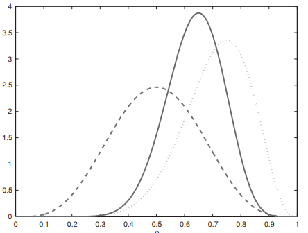
Figure 2.1 Prior (dashed line), scaled likelihood (dotted line), and posterior distribution (solid line) for the gambler’s ruin problem.
the posterior mean, that is,
$$
E[\boldsymbol{\theta} \mid \mathbf{x}]=\int \boldsymbol{\theta} f(\boldsymbol{\theta} \mid \mathbf{x}) \mathrm{d} \boldsymbol{\theta}
$$
or, in the univariate case, through a posterior median, that is,
$$
\theta_{\text {med }} \in{y: P(\theta \leq y \mid x)=1 / 2 ; P(\theta \geq y \mid x)=1 / 2}
$$
or through a posterior mode, that is
$$
\theta_{\text {mode }}=\arg \max f(\theta \mid \mathbf{x})
$$

随机过程代写

统计代写|应用随机过程代写Stochastic process代考|Bayesian analysis

在本章中，我们简要介绍了本书标题的第一部分，即贝叶斯分析，提供了本书其余部分使用的关键结果、方法和工具的摘要。大多数想法都是通过几个展示相关模型的工作示例来说明的。本章还设置了我们稍后将遵循的基本符号。

在过去的几年里，已经出版了许多涉及贝叶斯分析各个方面的书籍。本章末尾的讨论中引用了一些最相关的文献。然而，与这些书中的大多数相比，鉴于我们后来对随机过程的处理所强调的重点，我们将在此强调我们本书的两个核心问题，即决策和计算问题。

本章组织如下。一、在节2.2我们概述了推断、估计、假设检验和预测的贝叶斯方法的基础知识。我们还简要考虑了对先验分布的敏感性和使用非信息性先验分布的问题。在 2.3 节中，我们概述了贝叶斯决策分析。然后，在第 2.4 节中，我们简要回顾了贝叶斯计算方法。我们在第 2.5 节结束讨论。

统计代写|应用随机过程代写Stochastic process代考|Bayesian statistics

用于推理和预测的贝叶斯框架很容易描述。事实上，在概念层面上，贝叶斯方法的主要优势之一是基本思想易于实施。

特别是，统计学的典型目标之一是了解一个（或多个）参数，比如θ，它描述了一种感兴趣的随机现象。学习关于θ，我们将观察现象，收集数据样本，说X=(X1,X2,…,Xn)

并计算给定数据的条件密度或概率函数θ, 我们记为F(X∣θ). 这种联合密度，当被认为是θ, 通常被称为似然函数，通常表示为l(θ∣X)， 或者l(θ∣数据）当符号变得麻烦时。尽管在本书中并非总是如此，但由于随机过程产生的数据的内在依赖性，为了说明贝叶斯统计的主要思想，在本章中，我们通常假设X=(X1,…,Xn)给定（有条件地）独立同分布（CIID）θ.

除了似然函数，贝叶斯方法还考虑了有关参数的另一个信息来源θ. 通常，分析师可以访问外部信息来源，例如专家信息，可能基于过去的经验或以前的相关研究。该外部信息作为先验分布并入贝叶斯分析，F(θ).

先验和似然可以通过提供后验分布的贝叶斯定理组合F(θ∣X)，即参数的分布θ给定观察到的数据X,
F(θ∣X)=F(θ)F(X∣θ)∫F(θ)F(X∣θ)dθ∝F(θ)F(X∣θ)
后验分布总结了有关参数的所有可用信息，可用于解决所有标准统计问题，如点和区间估计、假设检验或预测。在本章中，我们将使用以下两个示例来说明这些问题。

统计代写|应用随机过程代写Stochastic process代考|Parameter estimation

作为使用后验分布的一个例子，我们可能对点估计感兴趣。这通常通过总结分布来解决，要么

图 2.1 赌徒破产问题的先验（虚线）、比例似然（虚线）和后验分布（实线）。
后验均值，即
和[θ∣X]=∫θF(θ∣X)dθ
或者，在单变量情况下，通过后中位数，即
θ和 ∈是:磷(θ≤是∣X)=1/2;磷(θ≥是∣X)=1/2
或通过后验模式，即
θ模式 =参数⁡最大限度F(θ∣X)

统计代写请认准statistics-lab™. statistics-lab™为您的留学生涯保驾护航。

金融工程代写

金融工程是使用数学技术来解决金融问题。金融工程使用计算机科学、统计学、经济学和应用数学领域的工具和知识来解决当前的金融问题，以及设计新的和创新的金融产品。

非参数统计代写

非参数统计指的是一种统计方法，其中不假设数据来自于由少数参数决定的规定模型；这种模型的例子包括正态分布模型和线性回归模型。

广义线性模型代考

广义线性模型（GLM）归属统计学领域，是一种应用灵活的线性回归模型。该模型允许因变量的偏差分布有除了正态分布之外的其它分布。

术语 广义线性模型（GLM）通常是指给定连续和/或分类预测因素的连续响应变量的常规线性回归模型。它包括多元线性回归，以及方差分析和方差分析（仅含固定效应）。

有限元方法代写

有限元方法（FEM）是一种流行的方法，用于数值解决工程和数学建模中出现的微分方程。典型的问题领域包括结构分析、传热、流体流动、质量运输和电磁势等传统领域。

有限元是一种通用的数值方法，用于解决两个或三个空间变量的偏微分方程（即一些边界值问题）。为了解决一个问题，有限元将一个大系统细分为更小、更简单的部分，称为有限元。这是通过在空间维度上的特定空间离散化来实现的，它是通过构建对象的网格来实现的：用于求解的数值域，它有有限数量的点。边界值问题的有限元方法表述最终导致一个代数方程组。该方法在域上对未知函数进行逼近。[1] 然后将模拟这些有限元的简单方程组合成一个更大的方程系统，以模拟整个问题。然后，有限元通过变化微积分使相关的误差函数最小化来逼近一个解决方案。

tatistics-lab作为专业的留学生服务机构，多年来已为美国、英国、加拿大、澳洲等留学热门地的学生提供专业的学术服务，包括但不限于Essay代写，Assignment代写，Dissertation代写，Report代写，小组作业代写，Proposal代写，Paper代写，Presentation代写，计算机作业代写，论文修改和润色，网课代做，exam代考等等。写作范围涵盖高中，本科，研究生等海外留学全阶段，辐射金融，经济学，会计学，审计学，管理学等全球99%专业科目。写作团队既有专业英语母语作者，也有海外名校硕博留学生，每位写作老师都拥有过硬的语言能力，专业的学科背景和学术写作经验。我们承诺100%原创，100%专业，100%准时，100%满意。

随机分析代写

随机微积分是数学的一个分支，对随机过程进行操作。它允许为随机过程的积分定义一个关于随机过程的一致的积分理论。这个领域是由日本数学家伊藤清在第二次世界大战期间创建并开始的。

时间序列分析代写

随机过程，是依赖于参数的一组随机变量的全体，参数通常是时间。 随机变量是随机现象的数量表现，其时间序列是一组按照时间发生先后顺序进行排列的数据点序列。通常一组时间序列的时间间隔为一恒定值（如1秒，5分钟，12小时，7天，1年），因此时间序列可以作为离散时间数据进行分析处理。研究时间序列数据的意义在于现实中，往往需要研究某个事物其随时间发展变化的规律。这就需要通过研究该事物过去发展的历史记录，以得到其自身发展的规律。

回归分析代写

多元回归分析渐进（Multiple Regression Analysis Asymptotics）属于计量经济学领域，主要是一种数学上的统计分析方法，可以分析复杂情况下各影响因素的数学关系，在自然科学、社会和经济学等多个领域内应用广泛。

MATLAB代写

MATLAB 是一种用于技术计算的高性能语言。它将计算、可视化和编程集成在一个易于使用的环境中，其中问题和解决方案以熟悉的数学符号表示。典型用途包括：数学和计算算法开发建模、仿真和原型制作数据分析、探索和可视化科学和工程图形应用程序开发，包括图形用户界面构建MATLAB 是一个交互式系统，其基本数据元素是一个不需要维度的数组。这使您可以解决许多技术计算问题，尤其是那些具有矩阵和向量公式的问题，而只需用 C 或 Fortran 等标量非交互式语言编写程序所需的时间的一小部分。MATLAB 名称代表矩阵实验室。MATLAB 最初的编写目的是提供对由 LINPACK 和 EISPACK 项目开发的矩阵软件的轻松访问，这两个项目共同代表了矩阵计算软件的最新技术。MATLAB 经过多年的发展，得到了许多用户的投入。在大学环境中，它是数学、工程和科学入门和高级课程的标准教学工具。在工业领域，MATLAB 是高效研究、开发和分析的首选工具。MATLAB 具有一系列称为工具箱的特定于应用程序的解决方案。对于大多数 MATLAB 用户来说非常重要，工具箱允许您学习和应用专业技术。工具箱是 MATLAB 函数（M 文件）的综合集合，可扩展 MATLAB 环境以解决特定类别的问题。可用工具箱的领域包括信号处理、控制系统、神经网络、模糊逻辑、小波、仿真等。

R语言代写	问卷设计与分析代写
PYTHON代写	回归分析与线性模型代写
MATLAB代写	方差分析与试验设计代写
STATA代写	机器学习/统计学习代写
SPSS代写	计量经济学代写
EVIEWS代写	时间序列分析代写
EXCEL代写	深度学习代写
SQL代写	各种数据建模与可视化代写

如果你也在 怎样代写应用随机过程Stochastic process这个学科遇到相关的难题，请随时右上角联系我们的24/7代写客服。

随机过程被定义为随机变量X={Xt:t∈T}的集合，定义在一个共同的概率空间上，时期内的控制和状态轨迹，以使性能指数最小化的过程。

statistics-lab™ 为您的留学生涯保驾护航 在代写应用随机过程Stochastic process方面已经树立了自己的口碑, 保证靠谱, 高质且原创的统计Statistics代写服务。我们的专家在代写应用随机过程Stochastic process代写方面经验极为丰富，各种代写应用随机过程Stochastic process相关的作业也就用不着说。

我们提供的应用随机过程Stochastic process及其相关学科的代写，服务范围广, 其中包括但不限于:

• Statistical Inference 统计推断
• Statistical Computing 统计计算
• Advanced Probability Theory 高等楖率论
• Advanced Mathematical Statistics 高等数理统计学
• (Generalized) Linear Models 广义线性模型
• Statistical Machine Learning 统计机器学习
• Longitudinal Data Analysis 纵向数据分析
• Foundations of Data Science 数据科学基础

统计代写|应用随机过程代写Stochastic process代考|Poisson process

Poisson processes are continuous time, discrete space processes that we shall analyze in detail in Chapter 5. Here, we shall distinguish between homogeneous and nonhomogeneous Poisson processes.

Definition 1.12: Suppose that the stochastic process $\left{X_{t}\right}_{t \in T}$ describes the number of events of a certain type produced until time t and has the following properties:

1. The number of events in nonoverlapping intervals are independent.
2. There is a constant $\lambda$ such that the probabilities of occurrence of events over ‘small’ intervals of duration $\Delta t$ are:

• $P$ (number of events in $(t, t+\Delta t]=1)=\lambda \Delta t+o(\Delta t)$.
• $P$ (number of events in $(t, t+\Delta t]>1)=o(\Delta t)$, where o( $\Delta t)$ is such that $o(\Delta t) / \Delta t \rightarrow 0$ when $\Delta t \rightarrow 0 .$

Then, we say that $\left{X_{t}\right}$ is an homogeneous Poisson process with parameter $\lambda$, char acterized by the fact that $X_{t} \sim P o(\lambda t)$.

For such a process, it can be proved that the times between successive events are IID random variables with distribution $\operatorname{Ex}(\lambda)$.

The Poisson process is a particular case of many important generic types of processes. Among others, it is an example of a renewal process, that is, a process describing the number of events of a phenomenon of interest occurring until a certain time such that the times between events are IID random variables (exponential in the case of the Poisson process). Poisson processes are also a special case of continuous time Markov chains, with transition probabilities $p_{i, i+1}=1, \forall i$ and $\lambda_{i}=\lambda$.
Nonhomogeneous Poisson processes
Nonhomogeneous Poisson processes are characterized by the intensity function $\lambda(t)$ or the mean function $m(t)=\int_{0}^{t} \lambda(s) \mathrm{d} s$; we consider, in general, a time-dependent intensity function but it could be space and space-time dependent as well. Note that, when $\lambda(t)=\lambda$, we have an homogeneous Poisson process. For a nonhomogeneous Poisson process, the number of events occurring in the interval $(t, t+s]$ will have a $\mathrm{Po}(m(t+s)-m(t))$ distribution.

统计代写|应用随机过程代写Stochastic process代考|Gaussian processes

The Gaussian process is continuous in both time and state spaces. Let $\left{X_{t}\right}$ be a stochastic process such that for any $n$ times $\left{t_{1}, t_{2}, \ldots, t_{n}\right}$ the joint distribution of $X_{t_{i}}, i=1,2, \ldots, n$, is $n$-variate normal. Then, the process is Gaussian. Moreover, if for any finite set of time instants $\left{t_{i}\right}, i=1,2, \ldots$ the random variables are mutually independent and $X_{t}$ is normally distributed for every $t$, we call it a purely random Gaussian process.

Because of the specific properties of the normal distribution, we may easily specify many properties of a Gaussian process. For example, if a Gaussian process is weakly stationary, then it is strictly stationary.

统计代写|应用随机过程代写Stochastic process代考|Inference, prediction, and decision-making

Given the key definitions and results concerning stochastic processes, we can now informally set up the statistical and decision-making problems that we shall deal with in the following chapters.

Clearly, stochastic processes will be characterized by their initial value and the values of their parameters, which may be finite or infinite dimensional.

Example 1.3: In the case of the gambler’s ruin problem of Example $1.2$ the process is parameterized by $p$, the probability of heads. More generally, for a stationary finite Markov chain model with states $1,2, \ldots, k$, the parameters will be the transition probabilities $\left(p_{11}, \ldots, p_{k, k}\right)$, where $p_{i j}$ satisfy that $p_{i j} \geq 0$ and $\sum_{j} p_{i j}=1$.

The AR(1) process of Example $1.1$ is parameterized through the parameters $\phi_{0}$ and $\phi_{1}$ –

A nonhomogeneous Poisson process with intensity function $\lambda(t)=M \beta t^{\beta-1}$, corresponding to a Power Law model, is a finite parametric model with parameters $(M, \beta)$.

A normal dynamic linear model (DLM) with univariate observations $X_{n}$, is described by
$$
\begin{aligned}
\theta_{0} \mid D_{0} & \sim \mathrm{N}\left(m_{0}, C_{0}\right) \
\theta_{n} \mid \theta_{n-1} & \sim \mathrm{N}\left(\boldsymbol{G}{n} \theta{n-1}, \boldsymbol{W}{n}\right) \ X{n} \mid \theta_{n} & \sim \mathrm{N}\left(F_{n}^{\prime} \theta_{n}, V_{n}\right)
\end{aligned}
$$
where, for each $n, F_{n}$ is a known vector of dimension $m \times 1, \boldsymbol{G}{n}$ is a known $m \times m$ matrix, $V{n}$ is a known variance, and $W_{n}$ is a known $m \times m$ variance matrix. The parameters are now $\left{\theta_{0}, \theta_{1}, \ldots\right}$.

随机过程代写

统计代写|应用随机过程代写Stochastic process代考|Poisson process

泊松过程是连续的时间、离散的空间过程，我们将在第 5 章详细分析。在这里，我们将区分齐次和非齐次泊松过程。

定义 1.12：假设随机过程\left{X_{t}\right}_{t \in T}\left{X_{t}\right}_{t \in T}描述了在时间 t 之前产生的某种类型的事件的数量，并具有以下属性：

1. 非重叠间隔中的事件数是独立的。
2. 有一个常数λ使得事件在“小”持续时间间隔内发生的概率Δ吨是：

• 磷（事件数(吨,吨+Δ吨]=1)=λΔ吨+这(Δ吨).
• 磷（事件数(吨,吨+Δ吨]>1)=这(Δ吨), 其中 o(Δ吨)是这样的这(Δ吨)/Δ吨→0什么时候Δ吨→0.

然后，我们说\left{X_{t}\right}\left{X_{t}\right}是具有参数的齐次 Poisson 过程λ, 特点是X吨∼磷这(λ吨).

对于这样的过程，可以证明连续事件之间的时间是具有分布的 IID 随机变量前任⁡(λ).

泊松过程是许多重要的通用过程类型的一个特例。其中，它是更新过程的一个示例，即描述在某个时间之前发生的感兴趣现象的事件数量的过程，使得事件之间的时间是 IID 随机变量（在 Poisson 的情况下为指数过程）。泊松过程也是连续时间马尔可夫链的特例，具有转移概率p一世,一世+1=1,∀一世和λ一世=λ.
非齐次泊松过程
非齐次泊松过程的特征是强度函数λ(吨)或平均函数米(吨)=∫0吨λ(s)ds; 一般来说，我们认为强度函数是时间相关的，但它也可能是空间和时空相关的。请注意，当λ(吨)=λ，我们有一个齐次泊松过程。对于非齐次 Poisson 过程，区间内发生的事件数(吨,吨+s]会有一个磷这(米(吨+s)−米(吨))分配。

统计代写|应用随机过程代写Stochastic process代考|Gaussian processes

高斯过程在时间和状态空间都是连续的。让\left{X_{t}\right}\left{X_{t}\right}是一个随机过程，使得对于任何n次\left{t_{1}, t_{2}, \ldots, t_{n}\right}\left{t_{1}, t_{2}, \ldots, t_{n}\right}的联合分布X吨一世,一世=1,2,…,n， 是n- 变化正常。然后，该过程是高斯的。此外，如果对于任何有限的时刻集\left{t_{i}\right}, i=1,2, \ldots\left{t_{i}\right}, i=1,2, \ldots随机变量相互独立且X吨正态分布于每个吨，我们称其为纯随机高斯过程。

由于正态分布的特殊性质，我们可以很容易地指定高斯过程的许多性质。例如，如果高斯过程是弱平稳的，则它是严格平稳的。

统计代写|应用随机过程代写Stochastic process代考|Inference, prediction, and decision-making

鉴于有关随机过程的关键定义和结果，我们现在可以非正式地设置我们将在接下来的章节中处理的统计和决策问题。

显然，随机过程的特征在于它们的初始值和它们的参数值，它们可能是有限维或无限维的。

例 1.3：以 Example 的赌徒破产问题为例1.2该过程由以下参数化p，正面的概率。更一般地，对于具有状态的平稳有限马尔可夫链模型1,2,…,ķ，参数将是转移概率(p11,…,pķ,ķ)， 在哪里p一世j满足p一世j≥0和∑jp一世j=1.

示例的 AR(1) 过程1.1通过参数参数化φ0和φ1 –

具有强度函数的非齐次 Poisson 过程λ(吨)=米b吨b−1，对应于幂律模型，是带参数的有限参数模型(米,b).

具有单变量观测值的正态动态线性模型 (DLM)Xn, 描述为
θ0∣D0∼ñ(米0,C0) θn∣θn−1∼ñ(Gnθn−1,在n) Xn∣θn∼ñ(Fn′θn,在n)
其中，对于每个n,Fn是一个已知的维度向量米×1,Gn是一个已知的米×米矩阵，在n是一个已知的方差，并且在n是一个已知的米×米方差矩阵。现在的参数是\left{\theta_{0}, \theta_{1}, \ldots\right}\left{\theta_{0}, \theta_{1}, \ldots\right}.

统计代写请认准statistics-lab™. statistics-lab™为您的留学生涯保驾护航。

金融工程代写

金融工程是使用数学技术来解决金融问题。金融工程使用计算机科学、统计学、经济学和应用数学领域的工具和知识来解决当前的金融问题，以及设计新的和创新的金融产品。

非参数统计代写

非参数统计指的是一种统计方法，其中不假设数据来自于由少数参数决定的规定模型；这种模型的例子包括正态分布模型和线性回归模型。

广义线性模型代考

广义线性模型（GLM）归属统计学领域，是一种应用灵活的线性回归模型。该模型允许因变量的偏差分布有除了正态分布之外的其它分布。

术语 广义线性模型（GLM）通常是指给定连续和/或分类预测因素的连续响应变量的常规线性回归模型。它包括多元线性回归，以及方差分析和方差分析（仅含固定效应）。

有限元方法代写

有限元方法（FEM）是一种流行的方法，用于数值解决工程和数学建模中出现的微分方程。典型的问题领域包括结构分析、传热、流体流动、质量运输和电磁势等传统领域。

有限元是一种通用的数值方法，用于解决两个或三个空间变量的偏微分方程（即一些边界值问题）。为了解决一个问题，有限元将一个大系统细分为更小、更简单的部分，称为有限元。这是通过在空间维度上的特定空间离散化来实现的，它是通过构建对象的网格来实现的：用于求解的数值域，它有有限数量的点。边界值问题的有限元方法表述最终导致一个代数方程组。该方法在域上对未知函数进行逼近。[1] 然后将模拟这些有限元的简单方程组合成一个更大的方程系统，以模拟整个问题。然后，有限元通过变化微积分使相关的误差函数最小化来逼近一个解决方案。

tatistics-lab作为专业的留学生服务机构，多年来已为美国、英国、加拿大、澳洲等留学热门地的学生提供专业的学术服务，包括但不限于Essay代写，Assignment代写，Dissertation代写，Report代写，小组作业代写，Proposal代写，Paper代写，Presentation代写，计算机作业代写，论文修改和润色，网课代做，exam代考等等。写作范围涵盖高中，本科，研究生等海外留学全阶段，辐射金融，经济学，会计学，审计学，管理学等全球99%专业科目。写作团队既有专业英语母语作者，也有海外名校硕博留学生，每位写作老师都拥有过硬的语言能力，专业的学科背景和学术写作经验。我们承诺100%原创，100%专业，100%准时，100%满意。

随机分析代写

随机微积分是数学的一个分支，对随机过程进行操作。它允许为随机过程的积分定义一个关于随机过程的一致的积分理论。这个领域是由日本数学家伊藤清在第二次世界大战期间创建并开始的。

时间序列分析代写

随机过程，是依赖于参数的一组随机变量的全体，参数通常是时间。 随机变量是随机现象的数量表现，其时间序列是一组按照时间发生先后顺序进行排列的数据点序列。通常一组时间序列的时间间隔为一恒定值（如1秒，5分钟，12小时，7天，1年），因此时间序列可以作为离散时间数据进行分析处理。研究时间序列数据的意义在于现实中，往往需要研究某个事物其随时间发展变化的规律。这就需要通过研究该事物过去发展的历史记录，以得到其自身发展的规律。

回归分析代写

多元回归分析渐进（Multiple Regression Analysis Asymptotics）属于计量经济学领域，主要是一种数学上的统计分析方法，可以分析复杂情况下各影响因素的数学关系，在自然科学、社会和经济学等多个领域内应用广泛。

MATLAB代写

MATLAB 是一种用于技术计算的高性能语言。它将计算、可视化和编程集成在一个易于使用的环境中，其中问题和解决方案以熟悉的数学符号表示。典型用途包括：数学和计算算法开发建模、仿真和原型制作数据分析、探索和可视化科学和工程图形应用程序开发，包括图形用户界面构建MATLAB 是一个交互式系统，其基本数据元素是一个不需要维度的数组。这使您可以解决许多技术计算问题，尤其是那些具有矩阵和向量公式的问题，而只需用 C 或 Fortran 等标量非交互式语言编写程序所需的时间的一小部分。MATLAB 名称代表矩阵实验室。MATLAB 最初的编写目的是提供对由 LINPACK 和 EISPACK 项目开发的矩阵软件的轻松访问，这两个项目共同代表了矩阵计算软件的最新技术。MATLAB 经过多年的发展，得到了许多用户的投入。在大学环境中，它是数学、工程和科学入门和高级课程的标准教学工具。在工业领域，MATLAB 是高效研究、开发和分析的首选工具。MATLAB 具有一系列称为工具箱的特定于应用程序的解决方案。对于大多数 MATLAB 用户来说非常重要，工具箱允许您学习和应用专业技术。工具箱是 MATLAB 函数（M 文件）的综合集合，可扩展 MATLAB 环境以解决特定类别的问题。可用工具箱的领域包括信号处理、控制系统、神经网络、模糊逻辑、小波、仿真等。

R语言代写	问卷设计与分析代写
PYTHON代写	回归分析与线性模型代写
MATLAB代写	方差分析与试验设计代写
STATA代写	机器学习/统计学习代写
SPSS代写	计量经济学代写
EVIEWS代写	时间序列分析代写
EXCEL代写	深度学习代写
SQL代写	各种数据建模与可视化代写

如果你也在 怎样代写应用随机过程Stochastic process这个学科遇到相关的难题，请随时右上角联系我们的24/7代写客服。

随机过程被定义为随机变量X={Xt:t∈T}的集合，定义在一个共同的概率空间上，时期内的控制和状态轨迹，以使性能指数最小化的过程。

statistics-lab™ 为您的留学生涯保驾护航 在代写应用随机过程Stochastic process方面已经树立了自己的口碑, 保证靠谱, 高质且原创的统计Statistics代写服务。我们的专家在代写应用随机过程Stochastic process代写方面经验极为丰富，各种代写应用随机过程Stochastic process相关的作业也就用不着说。

我们提供的应用随机过程Stochastic process及其相关学科的代写，服务范围广, 其中包括但不限于:

• Statistical Inference 统计推断
• Statistical Computing 统计计算
• Advanced Probability Theory 高等楖率论
• Advanced Mathematical Statistics 高等数理统计学
• (Generalized) Linear Models 广义线性模型
• Statistical Machine Learning 统计机器学习
• Longitudinal Data Analysis 纵向数据分析
• Foundations of Data Science 数据科学基础

统计代写|应用随机过程代写Stochastic process代考|Key concepts in stochastic processes

Stochastic processes model systems that evolve randomly in time, space or spacetime. This evolution will be described through an index $t \in T$. Consider a random experiment with sample space $\Omega$, endowed with a $\sigma$-algebra $\mathcal{F}$ and a base probability measure $P$. Associating numerical values with the elements of that space, we may define a family of random variables $\left{X_{t}, t \in T\right}$, which will be a stochastic process. This idea is formalized in our first definition that covers our object of interest in this book.

Definition 1.1: A stochastic process $\left{X_{t}, t \in T\right}$ is a collection of random variables $X_{t}$, indexed by a set $T$, taking values in a common measurable space $S$ endowed with an appropriate $\sigma$-algebra.
$T$ could be a set of times, when we have a temporal stochastic process; a set of spatial coordinates, when we have a spatial process; or a set of both time and spatial coordinates, when we deal with a spatio-temporal process. In this book, in general,

we shall focus on stochastic processes indexed by time, and will call $T$ the space of times. When $T$ is discrete, we shall say that the process is in discrete time and will denote time through $n$ and represent the process through $\left{X_{n}, n=0,1,2, \ldots\right}$. When $T$ is continuous, we shall say that the process is in continuous time. We shall usually assume that $T=[0, \infty)$ in this case. The values adopted by the process will be called the states of the process and will belong to the state space $S$. Again, $S$ may be either discrete or continuous.

At least two visions of a stochastic process can be given. First, for each $\omega \in \Omega$, we may rewrite $X_{t}(\omega)=g_{\omega}(t)$ and we have a function of $t$ which is a realization or a sample function of the stochastic process and describes a possible evolution of the process through time. Second, for any given $t, X_{t}$ is a random variable. To completely describe the stochastic process, we need a joint description of the family of random variables $\left{X_{t}, t \in T\right}$, not just the individual random variables. To do this, we may provide a description based on the joint distribution of the random variables at any discrete subset of times, that is, for any $\left{t_{1}, \ldots, t_{n}\right}$ with $t_{1}<\cdots<t_{n}$, and for any $\left{x_{1}, \ldots, x_{n}\right}$, we provide
$$
P\left(X_{t_{1}} \leq x_{1}, \ldots, X_{t_{n}} \leq x_{n}\right)
$$
Appropriate consistency conditions over these finite-dimensional families of distributions will ensure the definition of the stochastic process, via the Kolmogorov extension theorem, as in, for example, Øksendal (2003).

统计代写|应用随机过程代写Stochastic process代考|Main classes of stochastic processes

Except for the case of independence, the simplest dependence form among the random variables in a stochastic process is the Markovian one.

Definition 1.6: Consider a set of time instants $\left{t_{0}, t_{1}, \ldots, t_{n}, t\right}$ with $t_{0}<t_{1}<\cdots<$ $t_{n}<t$ and $t, t_{i} \in T$. A stochastic process $\left{X_{t}, t \in T\right}$ is Markovian if the distribution

of $X_{t}$ conditional on the values of $X_{t_{1}}, \ldots, X_{t_{n}}$ depends only on $X_{t_{n}}$, that is, the most recent known value of the process
$$
\begin{gathered}
P\left(X_{t} \leq x \mid X_{t_{x}} \leq x_{n}, X_{t_{n-1}} \leq x_{n-1}, \ldots, X_{t_{0}} \leq x_{0}\right) \
=P\left(X_{t} \leq x \mid X_{t_{n}} \leq x_{n}\right)=F\left(x_{n}, x ; t_{n}, t\right)
\end{gathered}
$$
As a consequence of the previous relation, we have
$$
F\left(x_{0}, x ; t_{0}, t_{0}+t\right)=\int_{y \in S} F(y, x ; \tau, t) \mathrm{d} F\left(x_{0}, y ; t_{0}, \tau\right)
$$
with $t_{0}<\taun_{1}>\cdots>n_{k}$, we have
$$
\begin{aligned}
P\left(X_{n}=j \mid X_{n_{1}}=i_{1}, X_{n_{2}}=i_{2}, \ldots, X_{n_{k}}=i_{n_{k}}\right) &=\
P\left(X_{n}=j \mid X_{n_{1}}=i_{1}\right) &=p_{i_{1} j}^{\left(n_{1}, n\right)}
\end{aligned}
$$
Using this property and taking $r$ such that $m<r<n$, we have
$$
\begin{aligned}
p_{i j}^{(m, n)} &=P\left(X_{n}=j \mid X_{m}=i\right) \
&=\sum_{k \in S} P\left(X_{n}=j \mid X_{r}=k\right) P\left(X_{r}=k \mid X_{m}=i\right)
\end{aligned}
$$
Equations (1.4) and (1.5) are called the Chapman-Kolmogorov equations for the continuous and discrete cases, respectively. In this book we shall refer to discrete state space Markov processes as Markov chains and will use the term Markov process to refer to processes with continuous state spaces and the Markovian property.

统计代写|应用随机过程代写Stochastic process代考|Discrete time Markov chains

Markov chains with discrete time space are an important class of stochastic processes whose analysis serves as a guide to the study of other more complex processes. The main features of such chains are outlined in the following text. Their full analysis is provided in Chapter 3 .

Consider a discrete state space Markov chain, $\left{X_{n}\right}$. Let $p_{i j}^{(m, n)}$ be defined as in (1.5), being the probability that the process is at time $n$ in $j$, when it was in $i$ at time $m$. If $n=m+1$, we have
$$
p_{i j}^{(m, m+1)}=P\left(X_{m+1}=j \mid X_{m}=i\right)
$$
which is known as the one-step transition probability. When $p_{i j}^{(m, m+1)}$ is independent of $m$, the process is stationary and the chain is called time homogeneous. Otherwise,

the process is called time inhomogeneous. Using the notation
$$
\begin{aligned}
&p_{i j}=P\left(X_{m+1}=j \mid X_{m}=i\right) \
&p_{i j}^{n}=P\left(X_{n+m}=j \mid X_{m}=i\right)
\end{aligned}
$$
for every $m$, the Chapman-Kolmogorov equations are now
$$
p_{i j}^{n+m}=\sum_{k \in S} p_{i k}^{n} p_{k j}^{m}
$$
for every $n, m \geq 0$ and $i, j$. The $n$-step transition probability matrix is defined as $\mathbf{P}^{(n)}$, with elements $p_{i j}^{n}$. Equation (1.6) is written $\mathbf{P}^{(n+m)}=\mathbf{P}^{(n)} \cdot \mathbf{P}^{(m)}$. These matrices fully characterize the transition behavior of an homogeneous Markov chain. When $n=1$, we shall usually write $\mathbf{P}$ instead of $\mathbf{P}^{(1)}$ and shall refer to the transition matrix instead of the one-step transition matrix.

随机过程代写

统计代写|应用随机过程代写Stochastic process代考|Key concepts in stochastic processes

随机过程模拟在时间、空间或时空中随机演化的系统。这种演变将通过一个索引来描述吨∈吨. 考虑一个带有样本空间的随机实验Ω, 具有σ-代数F和一个基本概率测度磷. 将数值与该空间的元素相关联，我们可以定义一系列随机变量\left{X_{t}, t \in T\right}\left{X_{t}, t \in T\right}，这将是一个随机过程。这个想法在我们的第一个定义中得到了形式化，该定义涵盖了我们在本书中感兴趣的对象。

定义 1.1：随机过程\left{X_{t}, t \in T\right}\left{X_{t}, t \in T\right}是随机变量的集合X吨, 由一组索引吨, 在一个共同的可测量空间中取值小号被赋予了适当的σ-代数。
吨可能是一组时间，当我们有一个时间随机过程时；一组空间坐标，当我们有一个空间过程时；或一组时间和空间坐标，当我们处理时空过程时。在本书中，一般来说，

我们将关注按时间索引的随机过程，并将调用吨时代的空间。什么时候吨是离散的，我们可以说这个过程是在离散时间中的，并且将表示通过的时间n并通过\left{X_{n}, n=0,1,2, \ldots\right}\left{X_{n}, n=0,1,2, \ldots\right}. 什么时候吨是连续的，我们可以说这个过程是在连续的时间内。我们通常会假设吨=[0,∞)在这种情况下。进程采用的值称为进程的状态，属于状态空间小号. 再次，小号可以是离散的或连续的。

至少可以给出随机过程的两种设想。首先，对于每个ω∈Ω, 我们可以重写X吨(ω)=Gω(吨)我们有一个函数吨它是随机过程的实现或样本函数，描述了该过程随时间的可能演变。其次，对于任何给定的吨,X吨是一个随机变量。为了完整描述随机过程，我们需要对随机变量族进行联合描述\left{X_{t}, t \in T\right}\left{X_{t}, t \in T\right}，而不仅仅是单个随机变量。为此，我们可以提供基于随机变量在任何离散时间子集的联合分布的描述，也就是说，对于任何\left{t_{1}, \ldots, t_{n}\right}\left{t_{1}, \ldots, t_{n}\right}和吨1<⋯<吨n，并且对于任何\left{x_{1}, \ldots, x_{n}\right}\left{x_{1}, \ldots, x_{n}\right}， 我们提供
磷(X吨1≤X1,…,X吨n≤Xn)
这些有限维分布族的适当一致性条件将确保通过 Kolmogorov 扩展定理定义随机过程，例如 Øksendal (2003)。

统计代写|应用随机过程代写Stochastic process代考|Main classes of stochastic processes

除了独立的情况，随机过程中随机变量之间最简单的依赖形式是马尔可夫。

定义 1.6：考虑一组时间点\left{t_{0}, t_{1}, \ldots, t_{n}, t\right}\left{t_{0}, t_{1}, \ldots, t_{n}, t\right}和吨0<吨1<⋯< 吨n<吨和吨,吨一世∈吨. 随机过程\left{X_{t}, t \in T\right}\left{X_{t}, t \in T\right}如果分布是马尔可夫

的X吨以价值为条件X吨1,…,X吨n只取决于X吨n，即过程的最新已知值
磷(X吨≤X∣X吨X≤Xn,X吨n−1≤Xn−1,…,X吨0≤X0) =磷(X吨≤X∣X吨n≤Xn)=F(Xn,X;吨n,吨)
由于前面的关系，我们有
F(X0,X;吨0,吨0+吨)=∫是∈小号F(是,X;τ,吨)dF(X0,是;吨0,τ)
和吨0<\ 年1>⋯>nķ， 我们有
磷(Xn=j∣Xn1=一世1,Xn2=一世2,…,Xnķ=一世nķ)= 磷(Xn=j∣Xn1=一世1)=p一世1j(n1,n)
使用此属性并采取r这样米<r<n， 我们有
p一世j(米,n)=磷(Xn=j∣X米=一世) =∑ķ∈小号磷(Xn=j∣Xr=ķ)磷(Xr=ķ∣X米=一世)
方程 (1.4) 和 (1.5) 分别称为连续和离散情况的 Chapman-Kolmogorov 方程。在本书中，我们将离散状态空间马尔可夫过程称为马尔可夫链，并将使用马尔可夫过程一词来指代具有连续状态空间和马尔可夫性质的过程。

统计代写|应用随机过程代写Stochastic process代考|Discrete time Markov chains

具有离散时间空间的马尔可夫链是一类重要的随机过程，其分析可作为研究其他更复杂过程的指南。下文概述了此类链的主要特征。第 3 章提供了他们的全面分析。

考虑一个离散状态空间马尔可夫链，\left{X_{n}\right}\left{X_{n}\right}. 让p一世j(米,n)在 (1.5) 中定义，是过程在时间上的概率n在j, 当它在一世有时米. 如果n=米+1， 我们有
p一世j(米,米+1)=磷(X米+1=j∣X米=一世)
这被称为一步转移概率。什么时候p一世j(米,米+1)独立于米，过程是平稳的，链称为时间齐次的。除此以外，

该过程称为时间不均匀。使用符号
p一世j=磷(X米+1=j∣X米=一世) p一世jn=磷(Xn+米=j∣X米=一世)
对于每个米, Chapman-Kolmogorov 方程现在是
p一世jn+米=∑ķ∈小号p一世ķnpķj米
对于每个n,米≥0和一世,j. 这n-step转移概率矩阵定义为磷(n), 有元素p一世jn. 方程（1.6）写成磷(n+米)=磷(n)⋅磷(米). 这些矩阵完全表征了齐次马尔可夫链的转变行为。什么时候n=1，我们通常会写成磷代替磷(1)并且应参考转移矩阵而不是一步转移矩阵。

统计代写请认准statistics-lab™. statistics-lab™为您的留学生涯保驾护航。

金融工程代写

金融工程是使用数学技术来解决金融问题。金融工程使用计算机科学、统计学、经济学和应用数学领域的工具和知识来解决当前的金融问题，以及设计新的和创新的金融产品。

非参数统计代写

非参数统计指的是一种统计方法，其中不假设数据来自于由少数参数决定的规定模型；这种模型的例子包括正态分布模型和线性回归模型。

广义线性模型代考

广义线性模型（GLM）归属统计学领域，是一种应用灵活的线性回归模型。该模型允许因变量的偏差分布有除了正态分布之外的其它分布。

术语 广义线性模型（GLM）通常是指给定连续和/或分类预测因素的连续响应变量的常规线性回归模型。它包括多元线性回归，以及方差分析和方差分析（仅含固定效应）。

有限元方法代写

有限元方法（FEM）是一种流行的方法，用于数值解决工程和数学建模中出现的微分方程。典型的问题领域包括结构分析、传热、流体流动、质量运输和电磁势等传统领域。

有限元是一种通用的数值方法，用于解决两个或三个空间变量的偏微分方程（即一些边界值问题）。为了解决一个问题，有限元将一个大系统细分为更小、更简单的部分，称为有限元。这是通过在空间维度上的特定空间离散化来实现的，它是通过构建对象的网格来实现的：用于求解的数值域，它有有限数量的点。边界值问题的有限元方法表述最终导致一个代数方程组。该方法在域上对未知函数进行逼近。[1] 然后将模拟这些有限元的简单方程组合成一个更大的方程系统，以模拟整个问题。然后，有限元通过变化微积分使相关的误差函数最小化来逼近一个解决方案。

tatistics-lab作为专业的留学生服务机构，多年来已为美国、英国、加拿大、澳洲等留学热门地的学生提供专业的学术服务，包括但不限于Essay代写，Assignment代写，Dissertation代写，Report代写，小组作业代写，Proposal代写，Paper代写，Presentation代写，计算机作业代写，论文修改和润色，网课代做，exam代考等等。写作范围涵盖高中，本科，研究生等海外留学全阶段，辐射金融，经济学，会计学，审计学，管理学等全球99%专业科目。写作团队既有专业英语母语作者，也有海外名校硕博留学生，每位写作老师都拥有过硬的语言能力，专业的学科背景和学术写作经验。我们承诺100%原创，100%专业，100%准时，100%满意。

随机分析代写

随机微积分是数学的一个分支，对随机过程进行操作。它允许为随机过程的积分定义一个关于随机过程的一致的积分理论。这个领域是由日本数学家伊藤清在第二次世界大战期间创建并开始的。

时间序列分析代写

随机过程，是依赖于参数的一组随机变量的全体，参数通常是时间。 随机变量是随机现象的数量表现，其时间序列是一组按照时间发生先后顺序进行排列的数据点序列。通常一组时间序列的时间间隔为一恒定值（如1秒，5分钟，12小时，7天，1年），因此时间序列可以作为离散时间数据进行分析处理。研究时间序列数据的意义在于现实中，往往需要研究某个事物其随时间发展变化的规律。这就需要通过研究该事物过去发展的历史记录，以得到其自身发展的规律。

回归分析代写

多元回归分析渐进（Multiple Regression Analysis Asymptotics）属于计量经济学领域，主要是一种数学上的统计分析方法，可以分析复杂情况下各影响因素的数学关系，在自然科学、社会和经济学等多个领域内应用广泛。

MATLAB代写

MATLAB 是一种用于技术计算的高性能语言。它将计算、可视化和编程集成在一个易于使用的环境中，其中问题和解决方案以熟悉的数学符号表示。典型用途包括：数学和计算算法开发建模、仿真和原型制作数据分析、探索和可视化科学和工程图形应用程序开发，包括图形用户界面构建MATLAB 是一个交互式系统，其基本数据元素是一个不需要维度的数组。这使您可以解决许多技术计算问题，尤其是那些具有矩阵和向量公式的问题，而只需用 C 或 Fortran 等标量非交互式语言编写程序所需的时间的一小部分。MATLAB 名称代表矩阵实验室。MATLAB 最初的编写目的是提供对由 LINPACK 和 EISPACK 项目开发的矩阵软件的轻松访问，这两个项目共同代表了矩阵计算软件的最新技术。MATLAB 经过多年的发展，得到了许多用户的投入。在大学环境中，它是数学、工程和科学入门和高级课程的标准教学工具。在工业领域，MATLAB 是高效研究、开发和分析的首选工具。MATLAB 具有一系列称为工具箱的特定于应用程序的解决方案。对于大多数 MATLAB 用户来说非常重要，工具箱允许您学习和应用专业技术。工具箱是 MATLAB 函数（M 文件）的综合集合，可扩展 MATLAB 环境以解决特定类别的问题。可用工具箱的领域包括信号处理、控制系统、神经网络、模糊逻辑、小波、仿真等。

R语言代写	问卷设计与分析代写
PYTHON代写	回归分析与线性模型代写
MATLAB代写	方差分析与试验设计代写
STATA代写	机器学习/统计学习代写
SPSS代写	计量经济学代写
EVIEWS代写	时间序列分析代写
EXCEL代写	深度学习代写
SQL代写	各种数据建模与可视化代写