标签: UCASF3F5

物理代写|天体物理学和天文学代写Astrophysics and Astronomy代考|ASTY221

如果你也在 怎样代写天体物理学和天文学Astrophysics and Astronomy这个学科遇到相关的难题,请随时右上角联系我们的24/7代写客服。

天文学和天体物理学是对太阳系以外的物体和现象的研究。这结合了理论模拟和用地面和航天器携带的仪器对天体发射的电磁辐射和高能粒子进行观察。

statistics-lab™ 为您的留学生涯保驾护航 在代写天体物理学和天文学Astrophysics and Astronomy方面已经树立了自己的口碑, 保证靠谱, 高质且原创的统计Statistics代写服务。我们的专家在代写天体物理学和天文学Astrophysics and Astronomy代写方面经验极为丰富,各种代写天体物理学和天文学Astrophysics and Astronomy相关的作业也就用不着说。

我们提供的天体物理学和天文学Astrophysics and Astronomy及其相关学科的代写,服务范围广, 其中包括但不限于:

  • Statistical Inference 统计推断
  • Statistical Computing 统计计算
  • Advanced Probability Theory 高等概率论
  • Advanced Mathematical Statistics 高等数理统计学
  • (Generalized) Linear Models 广义线性模型
  • Statistical Machine Learning 统计机器学习
  • Longitudinal Data Analysis 纵向数据分析
  • Foundations of Data Science 数据科学基础
物理代写|天体物理学和天文学代写Astrophysics and Astronomy代考|ASTY221

物理代写|天体物理学和天文学代写Astrophysics and Astronomy代考|Declination of the Sun

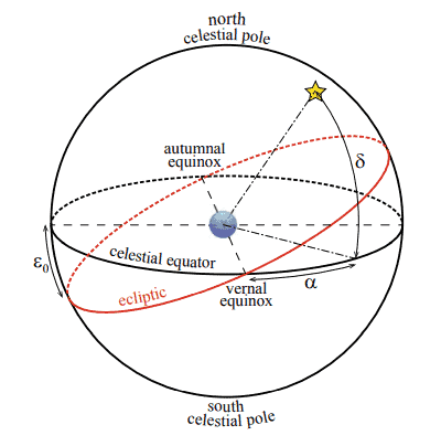
While the declination of stars is constant, the position of the Sun changes in the equatorial system over the period of a year. This is a consequence of the inclination of Earth’s rotation axis with respect to the direction perpendicular to the ecliptic, which is equal to $\epsilon_0=23.44^{\circ}$. The angle $\epsilon_0$ is called obliquity of the ecliptic. The annual variation of the declination of the Sun is approximately given by 3
$$
\delta_{\odot}=-\arcsin \left[\sin \epsilon_0 \cos \left(\frac{360^{\circ}}{365.24}(N+10)\right)\right]
$$

where $N$ is the difference in days starting from 1st January. So the first day of the year corresponds to $N=0$, and the last to $N=364$ (unless it is a leap year). The fraction $360^{\circ} / 365.24$ equals the change in the angular position of Earth per day, assuming a circular orbit. This is just the angular velocity $\omega$ of Earth’s orbital motion around the Sun in units of degrees per day. ${ }^4$

The Sun has zero declination at the equinoxes (intersection points of celestial equator and ecliptic) and reaches $\pm \epsilon_0$ at the solstices, where the rotation axis of the Earth is inclined towards or away from the Sun. The exact dates vary somewhat from year to year. In 2020, for instance, equinoxes were on 20th March and 22nd September and solstices on 20th June and 21st December (we neglect the exact times in the following). In Exercise $2.2$ you are asked to determine the corresponding values of $N$. For example, the 20th of June is the 172nd day of the year 2020. Counting from zero, we thus expect the maximum of the declination $\delta_{\odot}=\epsilon_0$ (first solstice) for $N=171$. Let us see if this is consistent with the approximation (2.1). The following Python code computes the declination $\delta_{\odot}$ based on this formula for a given value of $N$ :

The result
$$
\text { declination }=23.43 \text { deq }
$$
is close to the expected value of $23.44^{\circ}$. To implement Eq. (2.1), we use the sine, cosine, and arcsine functions from the math library. The arguments of these functions must be specified in radians. While the angular velocity is simply given by $2 \pi / 365.24 \mathrm{rad} / \mathrm{d}$ (see line 4 ), $\epsilon_0$ is converted into radians with the help of math.radians () in line 5. Both values are assigned to variables, which allows us to reuse them in subsequent parts of the program. Since the inverse function math. asin () returns an angle in radians, we need to convert delta into degrees when printing the result in line 9 (‘ $\mathrm{deg}$ ‘ is short for degrees).

物理代写|天体物理学和天文学代写Astrophysics and Astronomy代考|Diurnal Arc

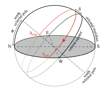
From the viewpoint of an observer on Earth, the apparent motion of an object on the celestial sphere follows an arc above the horizon, which is called diurnal arc (see Fig. 2.3). The time-dependent horizontal position of the object is measured by its hour angle $h$. An hour angle of $24^{\text {h }}$ corresponds to a full circle of $360^{\circ}$ parallel to the celestial equator (an example is the complete red circle in Fig. 2.3). For this reason, $h$ is can be equivalently expressed in degrees or radians. However, as we will see below, an hour angle of $1^{\mathrm{h}}$ is not equivalent to a time difference of one solar hour. By definition the hour angle is zero when the object reaches the highest altitude above the horizon (see also Exercise $2.4$ and Sect. 2.1.3). The hour angle corresponding to the setting time, when the object just vanishes beneath the horizon, is given by ${ }^6$

$$
\cos h_{\text {set }}=-\tan \delta \tan \phi,
$$
where $\delta$ is the declination of the object (see Sect. 2.1) and $\phi$ the latitude of the observer’s position on Earth. As a consequence, the variable $T=2 h_{\text {set }}$ measures the so-called sidereal time for which the object is in principle visible on the sky (stars are of course outshined by the Sun during daytime). It is also known as length of the diurnal are.

For example, let us consider the star Betelgeuse in the constellation of Orion. It is a red giant that is among the brightest stars on the sky. Its declination can be readily found with the help of astropy . coordinates, which offers a function that searches the name of an object in online databases: This tells us that the right ascension (ra) and declination (dec) of the object named Betelgeuse were found to be $88.79^{\circ}$ and $7.

物理代写|天体物理学和天文学代写Astrophysics and Astronomy代考|ASTY221

天体物理学和天文学代考

物理代写|天体物理学和天文学代写Astrophysics and Astronomy代考|Declination of the Sun

虽然恒星的偏角是恒定的,但一年中太阳在赤道系统中的位置会发生变化。这是地球自转轴相对于垂直于 黄道的方向倾斜的结果,等于 $\epsilon_0=23.44^{\circ}$. 角度 $\epsilon_0$ 称为黄道的倾角。太阳偏角的年变化大约为 3
$$
\delta_{\odot}=-\arcsin \left[\sin \epsilon_0 \cos \left(\frac{360^{\circ}}{365.24}(N+10)\right)\right]
$$
在哪里 $N$ 是从 1 月 1 日开始的天数差异。所以一年的第一天对应于 $N=0$ ,最后一个 $N=364$ (除非是 闰年)。分数 $360^{\circ} / 365.24$ 等于地球每天角位置的变化,假设为圆形轨道。这只是角速度 $\omega$ 地球围绕太 阳的轨道运动,以每天的度数为单位。4
太阳在春分点(天赤道和黄道的交点) 的赤纬为零,到达 $\pm \epsilon_0$ 在至点,地球的自转轴朝向或远离太阳倾 斜。确切的日期每年都有所不同。以2020年为例,春分是3月20日和9月22日,至日是6月20日和12月21 日 (以下具体时间略去) 。运动中 $2.2$ 你被要求确定相应的值 $N$. 例如, 6 月 20 日是 2020 年的第 172 天。从零开始计算,我们因此预计偏角的最大值 $\delta_{\odot}=\epsilon_0$ (初至) 为了 $N=171$. 让我们看看这是否与 近似 (2.1) 一致。以下 Python 代码计算偏角 $\delta_{\odot}$ 基于此公式的给定值 $N$ :
结果
$$
\text { declination }=23.43 \mathrm{deq}
$$
接近预期值 $23.44^{\circ}$. 实施方程式。(2.1),我们使用数学库中的正弦、余弦和反正弦函数。这些函数的参数 必须以弧度指定。虽然角速度简单地由下式给出 $2 \pi / 365.24 \mathrm{rad} / \mathrm{d}$ (见第 4 行), $\epsilon_0$ 在第 5 行的 math.radians() 的帮助下转换为弧度。这两个值都分配给变量,这使我们可以在程序的后续部分中重用它 们。由于反函数数学。 $\operatorname{asin}()$ 返回一个以弧度为单位的角度,我们需要在第 9 行打印结果时将 delta 转换 为度数 (‘deg’是学位的缩写)。

物理代写|天体物理学和天文学代写Astrophysics and Astronomy代考|Diurnal Arc

从地球上的观察者的角度来看,天球上物体的视运动沿着地平线上方的弧线运动,称为㡺弧(见图
2.3)。物体随时间变化的水平位置由其时角测量 $h$. 一个小时的角度 $24^{\mathrm{h}}$ 对应于一个完整的圆圈 $360^{\circ}$ 平 行于天赤道 (例如图 $2.3$ 中完整的红色圆圈) 。为此原因, $h$ 可以用度数或弧度等价地表示。然而,正如 我们将在下面看到的,小时角 $1^{\mathrm{h}}$ 不等于一个太阳时的时差。根据定义,当物体到达地平线以上的最高高 度时,时角为零 (另请参见练习 $2.4$ 和教派。2.1.3). 当物体刚刚消失在地平线下时,对应于设置时间的小 时角由下式给出 ${ }^6$
$$
\cos h_{\text {set }}=-\tan \delta \tan \phi,
$$
在哪里 $\delta$ 是物体的偏角(见第 $2.1$ 节) 和 $\phi$ 观察者在地球上的位置的纬度。因此,变量 $T=2 h_{\text {set }}$ 测量物 体在天空中原则上可见的所谓恒星时间(当然,白天星星比太阳更亮)。它也被称为昼夜长度。
例如,让我们考虑一下猎户座中的参宿四星。它是一颗红巨星,是天空中最亮的恒星之一。借助天体学可 以很容易地找到它的偏角。坐标,它提供了一个在在线数据库中搜索对象名称的功能:这告诉我们,名为 Betelgeuse 的对象的赤经 (ra) 和赤纬 (dec) 被发现是 $88.79^{\circ}$ 和 7 美元。

物理代写|天体物理学和天文学代写Astrophysics and Astronomy代考 请认准statistics-lab™

统计代写请认准statistics-lab™. statistics-lab™为您的留学生涯保驾护航。

金融工程代写

金融工程是使用数学技术来解决金融问题。金融工程使用计算机科学、统计学、经济学和应用数学领域的工具和知识来解决当前的金融问题,以及设计新的和创新的金融产品。

非参数统计代写

非参数统计指的是一种统计方法,其中不假设数据来自于由少数参数决定的规定模型;这种模型的例子包括正态分布模型和线性回归模型。

广义线性模型代考

广义线性模型(GLM)归属统计学领域,是一种应用灵活的线性回归模型。该模型允许因变量的偏差分布有除了正态分布之外的其它分布。

术语 广义线性模型(GLM)通常是指给定连续和/或分类预测因素的连续响应变量的常规线性回归模型。它包括多元线性回归,以及方差分析和方差分析(仅含固定效应)。

有限元方法代写

有限元方法(FEM)是一种流行的方法,用于数值解决工程和数学建模中出现的微分方程。典型的问题领域包括结构分析、传热、流体流动、质量运输和电磁势等传统领域。

有限元是一种通用的数值方法,用于解决两个或三个空间变量的偏微分方程(即一些边界值问题)。为了解决一个问题,有限元将一个大系统细分为更小、更简单的部分,称为有限元。这是通过在空间维度上的特定空间离散化来实现的,它是通过构建对象的网格来实现的:用于求解的数值域,它有有限数量的点。边界值问题的有限元方法表述最终导致一个代数方程组。该方法在域上对未知函数进行逼近。[1] 然后将模拟这些有限元的简单方程组合成一个更大的方程系统,以模拟整个问题。然后,有限元通过变化微积分使相关的误差函数最小化来逼近一个解决方案。

tatistics-lab作为专业的留学生服务机构,多年来已为美国、英国、加拿大、澳洲等留学热门地的学生提供专业的学术服务,包括但不限于Essay代写,Assignment代写,Dissertation代写,Report代写,小组作业代写,Proposal代写,Paper代写,Presentation代写,计算机作业代写,论文修改和润色,网课代做,exam代考等等。写作范围涵盖高中,本科,研究生等海外留学全阶段,辐射金融,经济学,会计学,审计学,管理学等全球99%专业科目。写作团队既有专业英语母语作者,也有海外名校硕博留学生,每位写作老师都拥有过硬的语言能力,专业的学科背景和学术写作经验。我们承诺100%原创,100%专业,100%准时,100%满意。

随机分析代写


随机微积分是数学的一个分支,对随机过程进行操作。它允许为随机过程的积分定义一个关于随机过程的一致的积分理论。这个领域是由日本数学家伊藤清在第二次世界大战期间创建并开始的。

时间序列分析代写

随机过程,是依赖于参数的一组随机变量的全体,参数通常是时间。 随机变量是随机现象的数量表现,其时间序列是一组按照时间发生先后顺序进行排列的数据点序列。通常一组时间序列的时间间隔为一恒定值(如1秒,5分钟,12小时,7天,1年),因此时间序列可以作为离散时间数据进行分析处理。研究时间序列数据的意义在于现实中,往往需要研究某个事物其随时间发展变化的规律。这就需要通过研究该事物过去发展的历史记录,以得到其自身发展的规律。

回归分析代写

多元回归分析渐进(Multiple Regression Analysis Asymptotics)属于计量经济学领域,主要是一种数学上的统计分析方法,可以分析复杂情况下各影响因素的数学关系,在自然科学、社会和经济学等多个领域内应用广泛。

MATLAB代写

MATLAB 是一种用于技术计算的高性能语言。它将计算、可视化和编程集成在一个易于使用的环境中,其中问题和解决方案以熟悉的数学符号表示。典型用途包括:数学和计算算法开发建模、仿真和原型制作数据分析、探索和可视化科学和工程图形应用程序开发,包括图形用户界面构建MATLAB 是一个交互式系统,其基本数据元素是一个不需要维度的数组。这使您可以解决许多技术计算问题,尤其是那些具有矩阵和向量公式的问题,而只需用 C 或 Fortran 等标量非交互式语言编写程序所需的时间的一小部分。MATLAB 名称代表矩阵实验室。MATLAB 最初的编写目的是提供对由 LINPACK 和 EISPACK 项目开发的矩阵软件的轻松访问,这两个项目共同代表了矩阵计算软件的最新技术。MATLAB 经过多年的发展,得到了许多用户的投入。在大学环境中,它是数学、工程和科学入门和高级课程的标准教学工具。在工业领域,MATLAB 是高效研究、开发和分析的首选工具。MATLAB 具有一系列称为工具箱的特定于应用程序的解决方案。对于大多数 MATLAB 用户来说非常重要,工具箱允许您学习应用专业技术。工具箱是 MATLAB 函数(M 文件)的综合集合,可扩展 MATLAB 环境以解决特定类别的问题。可用工具箱的领域包括信号处理、控制系统、神经网络、模糊逻辑、小波、仿真等。

R语言代写问卷设计与分析代写
PYTHON代写回归分析与线性模型代写
MATLAB代写方差分析与试验设计代写
STATA代写机器学习/统计学习代写
SPSS代写计量经济学代写
EVIEWS代写时间序列分析代写
EXCEL代写深度学习代写
SQL代写各种数据建模与可视化代写

物理代写|天体物理学和天文学代写Astrophysics and Astronomy代考|UCASF3F5

如果你也在 怎样代写天体物理学和天文学Astrophysics and Astronomy这个学科遇到相关的难题,请随时右上角联系我们的24/7代写客服。

天文学和天体物理学是对太阳系以外的物体和现象的研究。这结合了理论模拟和用地面和航天器携带的仪器对天体发射的电磁辐射和高能粒子进行观察。

statistics-lab™ 为您的留学生涯保驾护航 在代写天体物理学和天文学Astrophysics and Astronomy方面已经树立了自己的口碑, 保证靠谱, 高质且原创的统计Statistics代写服务。我们的专家在代写天体物理学和天文学Astrophysics and Astronomy代写方面经验极为丰富,各种代写天体物理学和天文学Astrophysics and Astronomy相关的作业也就用不着说。

我们提供的天体物理学和天文学Astrophysics and Astronomy及其相关学科的代写,服务范围广, 其中包括但不限于:

  • Statistical Inference 统计推断
  • Statistical Computing 统计计算
  • Advanced Probability Theory 高等概率论
  • Advanced Mathematical Statistics 高等数理统计学
  • (Generalized) Linear Models 广义线性模型
  • Statistical Machine Learning 统计机器学习
  • Longitudinal Data Analysis 纵向数据分析
  • Foundations of Data Science 数据科学基础
物理代写|天体物理学和天文学代写Astrophysics and Astronomy代考|UCASF3F5

物理代写|天体物理学和天文学代写Astrophysics and Astronomy代考|Control Structures

The computation of the orbital velocity of Earth in the previous section is a very simple example for the implementation of a numerical algorithm in Python. ${ }^9$ It involves the following steps:

  1. Initialisation of all data needed to perform the following computation.
  2. An exactly defined sequence of computational rules (usually based on mathematical formulas), unambiguously producing a result in a finite number of steps given the input from step 1.
  3. Output of the result.
    In our example, the definition of the variables radius and period provides the input, the expression for the orbital velocity is a computational rule, and the result assigned to the variable velocity is printed as output.

A common generalization of this simple scheme is the repeated execution of the same computational rule in a sequence of steps, where the outcome of one step is used as input for the next step. This is called iteration and will be explained in the remainder of this section. The independent application of the same operations to multiple elements of data is important when working with arrays, which will be introduced in Chap. 2.

Iteration requires a control structure for repeating the execution of a block of statements a given number of times or until a certain condition is met and the iteration terminates. Such a structure is called a loop. For example, let us consider the problem of summing up the first 100 natural numbers (this is a special case of an arithmetic series, in which each term differs by the previous one by a constant):
$$
s_n \equiv \sum_{k=1}^n k=1+2+3+\ldots+n
$$ The keywords for and in indicate that the loop counter $\mathrm{k}$ runs through all integers defined by range $(1, n+1)$, which means the sequence $1,2,3, \ldots, n$ in mathematical notation. It is a potential source of confusion that Python includes the start value 1 , but excludes the stop value $n+1$ in range $(1, n+1) .{ }^{10}$

物理代写|天体物理学和天文学代写Astrophysics and Astronomy代考|Working with Modules and Objects

Python offers a collection of useful tools in the Python Standard Library (see docs.python.org/3/library). Functions such as print () are part of the Standard Library. They are called built-in functions. Apart from that, many more optional

libraries (also called packages) are available. Depending on the Python distribution you use, you will find that some libraries are included and can be imported as shown below, while you might need to install others. ${ }^{16}$ Python libraries have a hierarchical modular structure. This means that you do not necessarily have to load a complete library, but you can access some part of a library, which can be a module, a submodule (i.e. a module within a module) or even individual names defined in a module. To get started, it will be sufficient to consider a module as a collection of definitions. By importing a module, you can use variables, functions, and classes (see below) defined in the module.

For example, important physical constants and conversion factors are defined in the constants module of the SciPy library (for more information, see www.scipy.org/about.html). A module can be loaded with the import command:
|import scipy.constants
To view an alphabetically ordered list of all names defined in this module, you can invoke dir (scipy. constants) (this works only after a module is imported). By scrolling through the list, you might notice the entry ‘gravitational_constant’. As the name suggests, this is the gravitational constant $G$. Try
2 print(scipy.constants.gravitational_constant)
which displays the value of $G$ in SI units:
$$
6.67408 e-11
$$
The same value is obtained via scipy.constants.G. Even so, an identifier composed of a library name in conjunction with a module and a variable name is rather cumbersome to use in programs. Alternatively, a module can be accessed via an alias: also displays the value of $G$. Here, const is a user-defined nickname for scipy. constants.

物理代写|天体物理学和天文学代写Astrophysics and Astronomy代考|UCASF3F5

天体物理学和天文学代考

物理代写|天体物理学和天文学代写Astrophysics and Astronomy代考|Control Structures

上一节中地球轨道速度的计算是用Python实现数值算法的一个非常简单的例子。 ${ }^9$ 它涉及以下步骤:

  1. 初始化执行以下计算所需的所有数据。
  2. 一个精确定义的计算规则序列(通常基于数学公式),在给定步骙 1 的输入的情况下,在有限的步 骤中明确地产生一个结果。
  3. 结果的输出。
    在我们的示例中,变量半径和周期的定义提供了输入,轨道速度的表达式是计算规则,分配给变量 速度的结果作为输出打印。
    这个简单方案的一个常见概括是在一系列步㡜中重复执行相同的计算规则,其中一步的结果用作下一步的 输入。这称为迭代,将在本节的其余部分进行解释。在使用数组时,将相同的操作独立应用于多个数据元 素非常重要,这将在第 1 章中介绍。2.
    迭代需要一个控制结构来重复执行一个语句块给定的次数,或者直到满足某个条件并且迭代终止。这样的 结构称为循环。例如,让我们考虑对前 100 个自然数求和的问题(这是算术级数的特例,其中每一项与 前一项相差一个常数):
    $$
    s_n \equiv \sum_{k=1}^n k=1+2+3+\ldots+n
    $$
    for和in关键字表示循环计数器k遍历范围定义的所有整数 $(1, n+1)$ ,这意味着序列 $1,2,3, \ldots, n$ 在数 学符号中。Python 包括起始值 1 但不包括停止值,这是一个潜在的混洧来源 $n+1$ 在范围内 $(1, n+1){ }^{10}$

物理代写|天体物理学和天文学代写Astrophysics and Astronomy代考|Working with Modules and Objects

Python 在 Python 标准库中提供了一系列有用的工具 (请参阅 docs.python.org/3/library) 。print() 等 函数是标准库的一部分。它们被称为内置函数。除此之外还有很多可选的
库 (也称为包) 可用。根据您使用的 Python 发行版,您会发现其中包含一些库并且可以如下所示导入, 而您可能需要安装其他库。 ${ }^{16}$ Python 库具有分层模块化结构。这意味着您不必加载完整的库,但您可以 访问库的某些部分,它可以是模块、子模块(即模块中的模块)甚至是模块中定义的单独名称。首先,将 模块视为定义的集合就足够了。通过导入模块,您可以使用模块中定义的变量、函数和类(见下文)。
例如,重要的物理常量和转换因子定义在 SciPy 库的常量模块中(有关更多信息,请参见 www.scipy.org/about.html) 。可以使用导入命令加载模块:
| import scipy.constants
要查看此模块中定义的所有名称的按字母顺序排列的列表,您可以调用 dir (scipy.constants) (这仅在导 入模块后有效)。通过滚动列表,您可能会注意到条目“gravitational_constant”。顾名思义,这就是万有 引力常数 $G$. 会试
2 print(scipy.constants.gravitational_constant)
显示值 $G$ 在 SI 单位中:
$$
6.67408 e-11
$$
通过 scipy.constants.G 获得相同的值。即便如此,由库名与模块名和变量名组成的标识符在程序中使用 起来还是相当麻烦。或者,可以通过别名访问模块:还显示 $G$. 这里,const 是 scipy 的用户自定义昵 称。常数。

物理代写|天体物理学和天文学代写Astrophysics and Astronomy代考 请认准statistics-lab™

统计代写请认准statistics-lab™. statistics-lab™为您的留学生涯保驾护航。

金融工程代写

金融工程是使用数学技术来解决金融问题。金融工程使用计算机科学、统计学、经济学和应用数学领域的工具和知识来解决当前的金融问题,以及设计新的和创新的金融产品。

非参数统计代写

非参数统计指的是一种统计方法,其中不假设数据来自于由少数参数决定的规定模型;这种模型的例子包括正态分布模型和线性回归模型。

广义线性模型代考

广义线性模型(GLM)归属统计学领域,是一种应用灵活的线性回归模型。该模型允许因变量的偏差分布有除了正态分布之外的其它分布。

术语 广义线性模型(GLM)通常是指给定连续和/或分类预测因素的连续响应变量的常规线性回归模型。它包括多元线性回归,以及方差分析和方差分析(仅含固定效应)。

有限元方法代写

有限元方法(FEM)是一种流行的方法,用于数值解决工程和数学建模中出现的微分方程。典型的问题领域包括结构分析、传热、流体流动、质量运输和电磁势等传统领域。

有限元是一种通用的数值方法,用于解决两个或三个空间变量的偏微分方程(即一些边界值问题)。为了解决一个问题,有限元将一个大系统细分为更小、更简单的部分,称为有限元。这是通过在空间维度上的特定空间离散化来实现的,它是通过构建对象的网格来实现的:用于求解的数值域,它有有限数量的点。边界值问题的有限元方法表述最终导致一个代数方程组。该方法在域上对未知函数进行逼近。[1] 然后将模拟这些有限元的简单方程组合成一个更大的方程系统,以模拟整个问题。然后,有限元通过变化微积分使相关的误差函数最小化来逼近一个解决方案。

tatistics-lab作为专业的留学生服务机构,多年来已为美国、英国、加拿大、澳洲等留学热门地的学生提供专业的学术服务,包括但不限于Essay代写,Assignment代写,Dissertation代写,Report代写,小组作业代写,Proposal代写,Paper代写,Presentation代写,计算机作业代写,论文修改和润色,网课代做,exam代考等等。写作范围涵盖高中,本科,研究生等海外留学全阶段,辐射金融,经济学,会计学,审计学,管理学等全球99%专业科目。写作团队既有专业英语母语作者,也有海外名校硕博留学生,每位写作老师都拥有过硬的语言能力,专业的学科背景和学术写作经验。我们承诺100%原创,100%专业,100%准时,100%满意。

随机分析代写


随机微积分是数学的一个分支,对随机过程进行操作。它允许为随机过程的积分定义一个关于随机过程的一致的积分理论。这个领域是由日本数学家伊藤清在第二次世界大战期间创建并开始的。

时间序列分析代写

随机过程,是依赖于参数的一组随机变量的全体,参数通常是时间。 随机变量是随机现象的数量表现,其时间序列是一组按照时间发生先后顺序进行排列的数据点序列。通常一组时间序列的时间间隔为一恒定值(如1秒,5分钟,12小时,7天,1年),因此时间序列可以作为离散时间数据进行分析处理。研究时间序列数据的意义在于现实中,往往需要研究某个事物其随时间发展变化的规律。这就需要通过研究该事物过去发展的历史记录,以得到其自身发展的规律。

回归分析代写

多元回归分析渐进(Multiple Regression Analysis Asymptotics)属于计量经济学领域,主要是一种数学上的统计分析方法,可以分析复杂情况下各影响因素的数学关系,在自然科学、社会和经济学等多个领域内应用广泛。

MATLAB代写

MATLAB 是一种用于技术计算的高性能语言。它将计算、可视化和编程集成在一个易于使用的环境中,其中问题和解决方案以熟悉的数学符号表示。典型用途包括:数学和计算算法开发建模、仿真和原型制作数据分析、探索和可视化科学和工程图形应用程序开发,包括图形用户界面构建MATLAB 是一个交互式系统,其基本数据元素是一个不需要维度的数组。这使您可以解决许多技术计算问题,尤其是那些具有矩阵和向量公式的问题,而只需用 C 或 Fortran 等标量非交互式语言编写程序所需的时间的一小部分。MATLAB 名称代表矩阵实验室。MATLAB 最初的编写目的是提供对由 LINPACK 和 EISPACK 项目开发的矩阵软件的轻松访问,这两个项目共同代表了矩阵计算软件的最新技术。MATLAB 经过多年的发展,得到了许多用户的投入。在大学环境中,它是数学、工程和科学入门和高级课程的标准教学工具。在工业领域,MATLAB 是高效研究、开发和分析的首选工具。MATLAB 具有一系列称为工具箱的特定于应用程序的解决方案。对于大多数 MATLAB 用户来说非常重要,工具箱允许您学习应用专业技术。工具箱是 MATLAB 函数(M 文件)的综合集合,可扩展 MATLAB 环境以解决特定类别的问题。可用工具箱的领域包括信号处理、控制系统、神经网络、模糊逻辑、小波、仿真等。

R语言代写问卷设计与分析代写
PYTHON代写回归分析与线性模型代写
MATLAB代写方差分析与试验设计代写
STATA代写机器学习/统计学习代写
SPSS代写计量经济学代写
EVIEWS代写时间序列分析代写
EXCEL代写深度学习代写
SQL代写各种数据建模与可视化代写

物理代写|天体物理学和天文学代写Astrophysics and Astronomy代考|Physics2151

如果你也在 怎样代写天体物理学和天文学Astrophysics and Astronomy这个学科遇到相关的难题,请随时右上角联系我们的24/7代写客服。

天文学和天体物理学是对太阳系以外的物体和现象的研究。这结合了理论模拟和用地面和航天器携带的仪器对天体发射的电磁辐射和高能粒子进行观察。

statistics-lab™ 为您的留学生涯保驾护航 在代写天体物理学和天文学Astrophysics and Astronomy方面已经树立了自己的口碑, 保证靠谱, 高质且原创的统计Statistics代写服务。我们的专家在代写天体物理学和天文学Astrophysics and Astronomy代写方面经验极为丰富,各种代写天体物理学和天文学Astrophysics and Astronomy相关的作业也就用不着说。

我们提供的天体物理学和天文学Astrophysics and Astronomy及其相关学科的代写,服务范围广, 其中包括但不限于:

  • Statistical Inference 统计推断
  • Statistical Computing 统计计算
  • Advanced Probability Theory 高等概率论
  • Advanced Mathematical Statistics 高等数理统计学
  • (Generalized) Linear Models 广义线性模型
  • Statistical Machine Learning 统计机器学习
  • Longitudinal Data Analysis 纵向数据分析
  • Foundations of Data Science 数据科学基础
物理代写|天体物理学和天文学代写Astrophysics and Astronomy代考|Physics2151

物理代写|天体物理学和天文学代写Astrophysics and Astronomy代考|Using Python

There is quite a variety of Python installations. Depending on the operating system of your computer, you might have some basic Python preinstalled. Typically, this is the case on Linux computers. However, you might find it rather cumbersome to use, especially if you are not well experienced with writing source code in elementary text editors and executing the code on the command line. What is more, installing additional packages typically requires administrative privileges. If you work, for example, in a computer lab it is likely that you do not have the necessary access rights. Apart from that, Python version 2.x (that is major version 2 with some subversion $\mathrm{x})$ is still in use, while this book is based on version 3.x.

Especially as a beginner, you will probably find it convenient to work with a a GUI (graphical user interface). Two popular choices for Python programming are Spyder and Jupyter. Spyder (www.spyder-ide.org) is a classical IDE (integrated development environment) which allows you to edit code, execute it and view the output in different frames. Jupyter (jupyter.org) can be operated via an arbitrary web browser. It allows you to run an interactive Python session with input and output cells (basically, just like the console-based ipython). Apart from input cells for typing Python source code, there are so-called markdown cells for writing headers and explanatory text. This allows you to use formatting similar to elementary HTML for webpages. A valuable feature is the incorporation of LaTeX to display mathematical expressions. The examples in this book can be downloaded as Jupyter notebooks and Python source code in zipped archives from uhh.de/phy-hs-pybook.

Since it depends on your personal preferences which software suits you best, we do not presume a particular GUI or Python distribution here. If you choose to work with Spyder or Jupyter, online documentation and tutorials will help you to install the software and to get started (browse the official documentation under docs.spyder-ide.org and jupyter-notebook.readthedocs.io/en/stable). For a comprehensive guideline, see also [1, appendices A and B]. A powerful all-in-one solution is Anaconda, a Python distribution and package manager that can be installed under Windows, macOS or Linux by any user (see docs.anaconda.com for more information). Anaconda provides a largely autonomous environment with all required components and libraries on a per-user basis. Of course, this comes at the cost of large resource consumption (in particular, watch your available disk space).

物理代写|天体物理学和天文学代写Astrophysics and Astronomy代考|Understanding Expressions and Assignments

Apart from printing messages on the screen, which is not particularly exciting by itself, Python can be used as a scientific calculator. Let us begin right away with an example from astronomy. Suppose we want to calculate the velocity at which Earth is moving along its orbit around the Sun. For simplicity, we treat the orbit as circular (in fact, it is elliptical with a small eccentricity of $0.017$ ). From the laws of circular motion it follows that we can simply calculate the velocity as the circumference $2 \pi r$ of the orbit divided by the period $P$, which happens to be one year for Earth. After having looked up the value of $\pi$, the orbital radius $r$ (i.e. the distance to the Sun) in $\mathrm{km}$, and the length of a year in seconds, ${ }^3$ we type
$$
12 * 3.14159 * 1.496 e 8 / 3.156 e 7
$$
and, once evaluated by Python, we obtain
$$
29.783388086185045
$$
for the orbital velocity in $\mathrm{km} / \mathrm{s}$. Line 1 is an example for a Python expression consisting of literal numbers and the arithmetic operators * and / for multiplication and division, respectively. The factor of two in the formula for the circumference is simply written as the integer 2 , while the number $\pi$ is approximately expressed in fixed-point decimal notation as $3.14159 . .^4$ The radius $r=1.496 \times 10^8 \mathrm{~km}$ is expressed as $1.496$ e8, which is a so-called floating point literal . The character e followed by an integer indicates the exponent of the leading digit in the decimal system. In this case, e8 corresponds to the factor $10^8$. Negative exponents are indicated by a minus sign after e. For example, $10^{-3}$ can be expressed as $1.0 e-3$ or just $1 e-3$ (inserting + for positive exponents is optional).

Of course, there is much more to Python than evaluating literal expressions like a calculator. To get an idea how this works, we turn the example shown above into a little Python program: Lines 1,2 , and 5 are examples for assignments. Each assignment binds the value of the expression on the right-hand side of the equality sign = to a name on the left-hand side.

物理代写|天体物理学和天文学代写Astrophysics and Astronomy代考|Physics2151

天体物理学和天文学代考

物理代写|天体物理学和天文学代写Astrophysics and Astronomy代考|Using Python

有相当多种 Python 安装。根据您计算机的操作系统,您可能预装了一些基本的 Python。通常,Linux 计算机就是这种情况。但是,您可能会发现它使用起来相当麻烦,尤其是如果您对在基本文本编辑器中编写源代码和在命令行上执行代码没有足够的经验。更重要的是,安装额外的包通常需要管理权限。例如,如果您在计算机实验室工作,您可能没有必要的访问权限。除此之外,Python 版本 2.x(即带有一些颠覆的主要版本 2X)仍在使用,而本书基于 3.x 版。

特别是作为初学者,您可能会发现使用 GUI(图形用户界面)很方便。Python 编程的两个流行选择是 Spyder 和 Jupyter。Spyder (www.spyder-ide.org) 是一个经典的 IDE(集成开发环境),它允许您编辑代码、执行它并在不同的框架中查看输出。Jupyter (jupyter.org) 可以通过任意网络浏览器运行。它允许您使用输入和输出单元运行交互式 Python 会话(基本上,就像基于控制台的 ipython 一样)。除了用于键入 Python 源代码的输入单元格外,还有用于编写标题和解释性文本的所谓降价单元格。这允许您对网页使用类似于基本 HTML 的格式。一个有价值的特性是结合了 LaTeX 来显示数学表达式。

由于最适合您的软件取决于您的个人喜好,因此我们不会在这里假定特定的 GUI 或 Python 发行版。如果您选择使用 Spyder 或 Jupyter,在线文档和教程将帮助您安装软件并开始使用(浏览 docs.spyder-ide.org 和 jupyter-notebook.readthedocs.io/en/stable 下的官方文档). 有关综合指南,另请参阅 [1,附录 A 和 B]。Anaconda 是一个功能强大的一体式解决方案,它是一个 Python 发行版和包管理器,任何用户都可以在 Windows、macOS 或 Linux 下安装(有关详细信息,请参阅 docs.anaconda.com)。Anaconda 为每个用户提供了一个高度自治的环境,其中包含所有必需的组件和库。当然,这是以大量资源消耗为代价的(特别是,

物理代写|天体物理学和天文学代写Astrophysics and Astronomy代考|Understanding Expressions and Assignments

除了在屏幕上打印消息本身并不是特别令人兴奋之外,Python 还可以用作科学计算器。让我们立即从天 文学的例子开始。假设我们要计算地球沿其绕太阳轨道运动的速度。为简单起见,我们将轨道视为圆形 (实际上,它是椭圆形,偏心率很小 $0.017$ ). 根据圆周运动定律,我们可以简单地将速度计算为圆周 $2 \pi r$ 轨道除以周期 $P$ ,这恰好是地球的一年。在查看了的值之后 $\pi$ ,轨道半径 $r$ (即到太阳的距离) 在 $\mathrm{km}$ ,以 及以秒为单位的一年的长度, ${ }^3$ 我们打字
$$
12 * 3.14159 * 1.496 e 8 / 3.156 e 7
$$
并且,一旦被 Python 评估,我们得到
$$
29.783388086185045
$$
对于轨道速度 $\mathrm{km} / \mathrm{s}$. 第 1 行是一个 Python 表达式的示例,该表达式由文字数字和分别用于乘法和除法 的算术运算符 * 和 / 组成。周长公式中的因数二简单地写为整数 2 ,而数 $\pi$ 用定点小数表示法近似表示为 $3.14159 . \mathrm{A}^4$ 半径 $r=1.496 \times 10^8 \mathrm{~km}$ 表示为 $1.496 \mathrm{e} 8$ ,也就是所谓的浮点字面量。字符 e 后跟一个整 数表示十进制系统中前导数字的指数。在这种情况下,e8 对应于因子 $10^8$. 负指数由 e 后的减号表示。例 如, $10^{-3}$ 可以表示为 $1.0 e-3$ 要不就 $1 e-3$ (为正指数揷入 $+$ 是可选的)。
当然,Python 的功能远不止像计算器那样计算文字表达式。为了了解这是如何工作的,我们将上面显示 的示例转换为一个小的 Python 程序: 第 1,2 和 5 行是赋值示例。每个赋值都将等号 = 右侧的表达式值绑 定到左侧的名称。

物理代写|天体物理学和天文学代写Astrophysics and Astronomy代考 请认准statistics-lab™

统计代写请认准statistics-lab™. statistics-lab™为您的留学生涯保驾护航。

金融工程代写

金融工程是使用数学技术来解决金融问题。金融工程使用计算机科学、统计学、经济学和应用数学领域的工具和知识来解决当前的金融问题,以及设计新的和创新的金融产品。

非参数统计代写

非参数统计指的是一种统计方法,其中不假设数据来自于由少数参数决定的规定模型;这种模型的例子包括正态分布模型和线性回归模型。

广义线性模型代考

广义线性模型(GLM)归属统计学领域,是一种应用灵活的线性回归模型。该模型允许因变量的偏差分布有除了正态分布之外的其它分布。

术语 广义线性模型(GLM)通常是指给定连续和/或分类预测因素的连续响应变量的常规线性回归模型。它包括多元线性回归,以及方差分析和方差分析(仅含固定效应)。

有限元方法代写

有限元方法(FEM)是一种流行的方法,用于数值解决工程和数学建模中出现的微分方程。典型的问题领域包括结构分析、传热、流体流动、质量运输和电磁势等传统领域。

有限元是一种通用的数值方法,用于解决两个或三个空间变量的偏微分方程(即一些边界值问题)。为了解决一个问题,有限元将一个大系统细分为更小、更简单的部分,称为有限元。这是通过在空间维度上的特定空间离散化来实现的,它是通过构建对象的网格来实现的:用于求解的数值域,它有有限数量的点。边界值问题的有限元方法表述最终导致一个代数方程组。该方法在域上对未知函数进行逼近。[1] 然后将模拟这些有限元的简单方程组合成一个更大的方程系统,以模拟整个问题。然后,有限元通过变化微积分使相关的误差函数最小化来逼近一个解决方案。

tatistics-lab作为专业的留学生服务机构,多年来已为美国、英国、加拿大、澳洲等留学热门地的学生提供专业的学术服务,包括但不限于Essay代写,Assignment代写,Dissertation代写,Report代写,小组作业代写,Proposal代写,Paper代写,Presentation代写,计算机作业代写,论文修改和润色,网课代做,exam代考等等。写作范围涵盖高中,本科,研究生等海外留学全阶段,辐射金融,经济学,会计学,审计学,管理学等全球99%专业科目。写作团队既有专业英语母语作者,也有海外名校硕博留学生,每位写作老师都拥有过硬的语言能力,专业的学科背景和学术写作经验。我们承诺100%原创,100%专业,100%准时,100%满意。

随机分析代写


随机微积分是数学的一个分支,对随机过程进行操作。它允许为随机过程的积分定义一个关于随机过程的一致的积分理论。这个领域是由日本数学家伊藤清在第二次世界大战期间创建并开始的。

时间序列分析代写

随机过程,是依赖于参数的一组随机变量的全体,参数通常是时间。 随机变量是随机现象的数量表现,其时间序列是一组按照时间发生先后顺序进行排列的数据点序列。通常一组时间序列的时间间隔为一恒定值(如1秒,5分钟,12小时,7天,1年),因此时间序列可以作为离散时间数据进行分析处理。研究时间序列数据的意义在于现实中,往往需要研究某个事物其随时间发展变化的规律。这就需要通过研究该事物过去发展的历史记录,以得到其自身发展的规律。

回归分析代写

多元回归分析渐进(Multiple Regression Analysis Asymptotics)属于计量经济学领域,主要是一种数学上的统计分析方法,可以分析复杂情况下各影响因素的数学关系,在自然科学、社会和经济学等多个领域内应用广泛。

MATLAB代写

MATLAB 是一种用于技术计算的高性能语言。它将计算、可视化和编程集成在一个易于使用的环境中,其中问题和解决方案以熟悉的数学符号表示。典型用途包括:数学和计算算法开发建模、仿真和原型制作数据分析、探索和可视化科学和工程图形应用程序开发,包括图形用户界面构建MATLAB 是一个交互式系统,其基本数据元素是一个不需要维度的数组。这使您可以解决许多技术计算问题,尤其是那些具有矩阵和向量公式的问题,而只需用 C 或 Fortran 等标量非交互式语言编写程序所需的时间的一小部分。MATLAB 名称代表矩阵实验室。MATLAB 最初的编写目的是提供对由 LINPACK 和 EISPACK 项目开发的矩阵软件的轻松访问,这两个项目共同代表了矩阵计算软件的最新技术。MATLAB 经过多年的发展,得到了许多用户的投入。在大学环境中,它是数学、工程和科学入门和高级课程的标准教学工具。在工业领域,MATLAB 是高效研究、开发和分析的首选工具。MATLAB 具有一系列称为工具箱的特定于应用程序的解决方案。对于大多数 MATLAB 用户来说非常重要,工具箱允许您学习应用专业技术。工具箱是 MATLAB 函数(M 文件)的综合集合,可扩展 MATLAB 环境以解决特定类别的问题。可用工具箱的领域包括信号处理、控制系统、神经网络、模糊逻辑、小波、仿真等。

R语言代写问卷设计与分析代写
PYTHON代写回归分析与线性模型代写
MATLAB代写方差分析与试验设计代写
STATA代写机器学习/统计学习代写
SPSS代写计量经济学代写
EVIEWS代写时间序列分析代写
EXCEL代写深度学习代写
SQL代写各种数据建模与可视化代写