
如果你也在 怎样代写热力学Thermodynamics 这个学科遇到相关的难题,请随时右上角联系我们的24/7代写客服。热力学Thermodynamics是物理学的一个分支,涉及热、功和温度,以及它们与能量、熵以及物质和辐射的物理特性的关系。这些数量的行为受热力学四大定律的制约,这些定律使用可测量的宏观物理量来传达定量描述,但可以用统计力学的微观成分来解释。热力学适用于科学和工程中的各种主题,特别是物理化学、生物化学、化学工程和机械工程,但也适用于其他复杂领域,如气象学。
热力学Thermodynamics从历史上看,热力学的发展源于提高早期蒸汽机效率的愿望,特别是通过法国物理学家萨迪-卡诺(1824年)的工作,他认为发动机的效率是可以帮助法国赢得拿破仑战争的关键。苏格兰-爱尔兰物理学家开尔文勋爵在1854年首次提出了热力学的简明定义,其中指出:”热力学是关于热与作用在身体相邻部分之间的力的关系,以及热与电的关系的课题。” 鲁道夫-克劳修斯重述了被称为卡诺循环的卡诺原理,为热学理论提供了更真实、更健全的基础。他最重要的论文《论热的运动力》发表于1850年,首次提出了热力学的第二定律。1865年,他提出了熵的概念。1870年,他提出了适用于热的维拉尔定理。
statistics-lab™ 为您的留学生涯保驾护航 在代写热力学thermodynamics方面已经树立了自己的口碑, 保证靠谱, 高质且原创的统计Statistics代写服务。我们的专家在代写热力学thermodynamics代写方面经验极为丰富,各种代写热力学thermodynamics相关的作业也就用不着说。
物理代写|热力学代写thermodynamics代考|Looking at entropy on a macroscopic level
On a macroscopic level, entropy is associated with the amount of energy in a system that is transferred by heat and isn’t used for doing work. For example, when a system (which could simply be a hot cup of tea sitting on your kitchen table) has an intemally reversible change in energy by a small amount of heat transfer $(\delta Q)$, the change in entropy $(d S)$, is equal to the heat transfer in the system divided by the absolute temperature $(T)$ of the system boundary. Mathematically, this definition of entropy is written like this:
$$
d S=\left(\frac{\delta Q}{T}\right)_{\text {im laer: }}
$$
The units for entropy on a per unit mass basis are kilojoules per kilogramKelvin $(\mathrm{kJ} / \mathrm{kg}-\mathrm{K})$.
The system boundary separates the system from its environment or surroundings. If you define the tea in the cup as the system, the cup itself can be considered the boundary, and the kitchen can be considered the surroundings.
An internally reversible change in energy means the system can go back to its original state if the process goes in the reverse direction. This concept is an idealization of real heat-transfer processes and assumes the temperature of the system and the surroundings are the same during heat transfer. In the real world, heat transfer requires a temperature difference between two objects. As the temperature difference between two objects approaches zero, the heat transfer rate between them decreases. It may require a very long time or a very large area to transfer heat between two objects to the point where it becomes impractical.
In real systems, there are always irreversibilities, such as friction, sudden expansion of a gas, or heat transfer with a temperature difference. The entropy change in a system having a real process is always greater than that of an internally reversible process, which means the entropy change for a system with a real irreversible process is expressed by the following inequality:
$$
d S_{\text {irrev }}>\left(\frac{\delta Q}{T}\right)_{\text {tint } \mathrm{Rev} \text {. }}
$$
物理代写|热力学代写thermodynamics代考|Working with T-s Diagrams
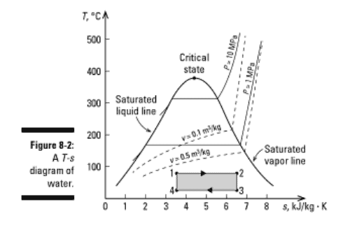
The temperature-entropy, or $T$-s, diagram helps you visualize a process with respect to the second law of thermodynamics; much like the $P-v$ and $T-v$ property diagrams I discuss in Chapter 3 help you grasp the first law of thermodynamics. Figure $8-2$ shows the $T$ s diagram of water. The diagram shows the saturated liquid and saturated vapor lines in the shape of a dome. Lines of constant pressure (for $P=1$ and 10 megapascals) and constant volume (for $v=0.1$ and 0.5 cubic meter per kilogram) on the diagram give you a sense of how constant pressure or constant volume processes may follow along these paths. You usually don’t find pressure-entropy, or P-s, diagrams in thermodynamics books, because they’re not as useful as the $T$-s diagram.
You can find the heat transfer for an internally reversible process by rearranging the equation used to define entropy (see the section “Looking at entropy on a macroscopic level”) and integrating it like this:
$$
Q_{\ln . \text { Rev. }}=\int_1^2 T d S
$$
From this equation, you see that heat transfer $(Q)$ is related only to temperature and entropy and equals the area under an internally reversible process curve drawn on a $T$-s diagram. To integrate this equation, you need the relationship between temperature and entropy for an internally reversible process. For example, a constant temperature process from States 1 to 2 at 75 degrees Celsius is shown in Figure 8-2. The entropy at States 1 and 2 is 3.5 and 6.5 kilojoules per kilogram-Kelvin, respectively. Integrating a constant temperature process gives the following equation for calculating heat transfer:
$$
Q=T \cdot \Delta S \text { or } q=T\left(s_2-s_1\right)
$$
As I discuss in Chapter 2, equations written with lowercase variables are on a unit mass basis (intensive form), whereas equations written with uppercase variables (extensive form) are used when the mass of the system is known.
You can calculate the heat transfer of an ideal reversible process, using absolute temperature. The result of this calculation is as follows:
$$
q=\left(75^{\circ} \mathrm{C}+273\right) \mathrm{K}(6.5-3.5) \mathrm{kJ} / \mathrm{kg} \cdot \mathrm{K}=1,044 \mathrm{~kJ} / \mathrm{kg}
$$
When heat is added to the system, it has an increase in entropy. When heat is removed from the system, it has a decrease in entropy, as shown from States 3 to 4 in Figure 8-2. For the isothermal process at 25 degrees Celsius from States 3 to 4 , you calculate the heat removed in a reversible process by using this equation:
$$
q=T\left(s_4-s_3\right)
$$
Substituting in the values for this equation gives the heat removed:
$$
q=\left(25^{\circ} \mathrm{C}+273\right) \mathrm{K}(3.5-6.5) \mathrm{kJ} / \mathrm{kg} \cdot \mathrm{K}=-894 \mathrm{~kJ} / \mathrm{kg}
$$
热力学代写
物理代写|热力学代写thermodynamics代考|Looking at entropy on a macroscopic level
宏观层面上,熵与系统中通过热传递而不用于做功的能量有关。例如,当一个系统(可以是你厨房桌子上的一杯热茶)有一个内部可逆的能量变化,通过少量的热量传递$(\delta Q)$,熵变$(d S)$,等于系统的热量传递除以系统边界的绝对温度$(T)$。在数学上,熵的定义是这样写的:
$$
d S=\left(\frac{\delta Q}{T}\right)_{\text {im laer: }}
$$
熵在单位质量基础上的单位是千焦每千克开尔文$(\mathrm{kJ} / \mathrm{kg}-\mathrm{K})$。
系统边界将系统与其环境或周围环境分开。如果你把杯子里的茶定义为系统,杯子本身可以被认为是边界,厨房可以被认为是环境。
内部可逆的能量变化意味着如果过程向相反的方向进行,系统可以回到原来的状态。这个概念是对实际传热过程的理想化,并假设在传热过程中系统和周围环境的温度是相同的。在现实世界中,传热需要两个物体之间的温差。当两个物体之间的温差趋近于零时,它们之间的传热速率减小。在两个物体之间传递热量可能需要很长时间或很大的面积,以至于变得不切实际。
在真实的系统中,总是存在着不可逆性,例如摩擦、气体的突然膨胀或有温差的热传递。真实过程系统的熵变总是大于内部可逆过程系统的熵变,这意味着真实不可逆过程系统的熵变可以用下面的不等式表示:
$$
d S_{\text {irrev }}>\left(\frac{\delta Q}{T}\right)_{\text {tint } \mathrm{Rev} \text {. }}
$$
物理代写|热力学代写thermodynamics代考|Working with T-s Diagrams
温度-熵,或$T$ -s,图表可以帮助你直观地看到热力学第二定律的过程;就像我在第三章讨论的$P-v$和$T-v$属性图一样,可以帮助你掌握热力学第一定律。图$8-2$显示了水的$T$ s图。该图显示了圆顶形状的饱和液体和饱和蒸汽线。图上的恒压线(对于$P=1$和10兆帕斯卡)和恒容线(对于$v=0.1$和每公斤0.5立方米)可以让您了解恒压或恒容过程如何沿着这些路径进行。你通常在热力学书上找不到压力-熵图,或者P-s图,因为它们没有$T$ -s图有用。
你可以通过重新排列用于定义熵的方程(参见“在宏观层面上观察熵”一节)并像这样积分来找到内部可逆过程的传热:
$$
Q_{\ln . \text { Rev. }}=\int_1^2 T d S
$$
从这个方程,你看到传热$(Q)$只与温度和熵有关,等于在$T$ -s图上绘制的内部可逆过程曲线下的面积。要对这个方程积分,你需要知道内部可逆过程的温度和熵的关系。例如,在75摄氏度下从状态1到状态2的恒温过程如图8-2所示。状态1和状态2的熵分别是3.5和6.5千焦耳每千克开尔文。对恒温过程积分得到传热计算公式如下:
$$
Q=T \cdot \Delta S \text { or } q=T\left(s_2-s_1\right)
$$
正如我在第2章中讨论的,用小写变量写的方程是基于单位质量的(密集形式),而用大写变量写的方程(扩展形式)是在系统质量已知的情况下使用的。
你可以用绝对温度来计算理想可逆过程的传热。计算结果如下:
$$
q=\left(75^{\circ} \mathrm{C}+273\right) \mathrm{K}(6.5-3.5) \mathrm{kJ} / \mathrm{kg} \cdot \mathrm{K}=1,044 \mathrm{~kJ} / \mathrm{kg}
$$
当热量加入系统时,熵增加。当热量从系统中移出时,熵会减少,如图8-2中状态3到状态4所示。对于从状态3到状态4在25摄氏度的等温过程,你可以用这个方程计算可逆过程中释放的热量:
$$
q=T\left(s_4-s_3\right)
$$
代入这个方程的值,得到了去除的热量:
$$
q=\left(25^{\circ} \mathrm{C}+273\right) \mathrm{K}(3.5-6.5) \mathrm{kJ} / \mathrm{kg} \cdot \mathrm{K}=-894 \mathrm{~kJ} / \mathrm{kg}
$$

统计代写请认准statistics-lab™. statistics-lab™为您的留学生涯保驾护航。
金融工程代写
金融工程是使用数学技术来解决金融问题。金融工程使用计算机科学、统计学、经济学和应用数学领域的工具和知识来解决当前的金融问题,以及设计新的和创新的金融产品。
非参数统计代写
非参数统计指的是一种统计方法,其中不假设数据来自于由少数参数决定的规定模型;这种模型的例子包括正态分布模型和线性回归模型。
广义线性模型代考
广义线性模型(GLM)归属统计学领域,是一种应用灵活的线性回归模型。该模型允许因变量的偏差分布有除了正态分布之外的其它分布。
术语 广义线性模型(GLM)通常是指给定连续和/或分类预测因素的连续响应变量的常规线性回归模型。它包括多元线性回归,以及方差分析和方差分析(仅含固定效应)。
有限元方法代写
有限元方法(FEM)是一种流行的方法,用于数值解决工程和数学建模中出现的微分方程。典型的问题领域包括结构分析、传热、流体流动、质量运输和电磁势等传统领域。
有限元是一种通用的数值方法,用于解决两个或三个空间变量的偏微分方程(即一些边界值问题)。为了解决一个问题,有限元将一个大系统细分为更小、更简单的部分,称为有限元。这是通过在空间维度上的特定空间离散化来实现的,它是通过构建对象的网格来实现的:用于求解的数值域,它有有限数量的点。边界值问题的有限元方法表述最终导致一个代数方程组。该方法在域上对未知函数进行逼近。[1] 然后将模拟这些有限元的简单方程组合成一个更大的方程系统,以模拟整个问题。然后,有限元通过变化微积分使相关的误差函数最小化来逼近一个解决方案。
tatistics-lab作为专业的留学生服务机构,多年来已为美国、英国、加拿大、澳洲等留学热门地的学生提供专业的学术服务,包括但不限于Essay代写,Assignment代写,Dissertation代写,Report代写,小组作业代写,Proposal代写,Paper代写,Presentation代写,计算机作业代写,论文修改和润色,网课代做,exam代考等等。写作范围涵盖高中,本科,研究生等海外留学全阶段,辐射金融,经济学,会计学,审计学,管理学等全球99%专业科目。写作团队既有专业英语母语作者,也有海外名校硕博留学生,每位写作老师都拥有过硬的语言能力,专业的学科背景和学术写作经验。我们承诺100%原创,100%专业,100%准时,100%满意。
随机分析代写
随机微积分是数学的一个分支,对随机过程进行操作。它允许为随机过程的积分定义一个关于随机过程的一致的积分理论。这个领域是由日本数学家伊藤清在第二次世界大战期间创建并开始的。
时间序列分析代写
随机过程,是依赖于参数的一组随机变量的全体,参数通常是时间。 随机变量是随机现象的数量表现,其时间序列是一组按照时间发生先后顺序进行排列的数据点序列。通常一组时间序列的时间间隔为一恒定值(如1秒,5分钟,12小时,7天,1年),因此时间序列可以作为离散时间数据进行分析处理。研究时间序列数据的意义在于现实中,往往需要研究某个事物其随时间发展变化的规律。这就需要通过研究该事物过去发展的历史记录,以得到其自身发展的规律。
回归分析代写
多元回归分析渐进(Multiple Regression Analysis Asymptotics)属于计量经济学领域,主要是一种数学上的统计分析方法,可以分析复杂情况下各影响因素的数学关系,在自然科学、社会和经济学等多个领域内应用广泛。
MATLAB代写
MATLAB 是一种用于技术计算的高性能语言。它将计算、可视化和编程集成在一个易于使用的环境中,其中问题和解决方案以熟悉的数学符号表示。典型用途包括:数学和计算算法开发建模、仿真和原型制作数据分析、探索和可视化科学和工程图形应用程序开发,包括图形用户界面构建MATLAB 是一个交互式系统,其基本数据元素是一个不需要维度的数组。这使您可以解决许多技术计算问题,尤其是那些具有矩阵和向量公式的问题,而只需用 C 或 Fortran 等标量非交互式语言编写程序所需的时间的一小部分。MATLAB 名称代表矩阵实验室。MATLAB 最初的编写目的是提供对由 LINPACK 和 EISPACK 项目开发的矩阵软件的轻松访问,这两个项目共同代表了矩阵计算软件的最新技术。MATLAB 经过多年的发展,得到了许多用户的投入。在大学环境中,它是数学、工程和科学入门和高级课程的标准教学工具。在工业领域,MATLAB 是高效研究、开发和分析的首选工具。MATLAB 具有一系列称为工具箱的特定于应用程序的解决方案。对于大多数 MATLAB 用户来说非常重要,工具箱允许您学习和应用专业技术。工具箱是 MATLAB 函数(M 文件)的综合集合,可扩展 MATLAB 环境以解决特定类别的问题。可用工具箱的领域包括信号处理、控制系统、神经网络、模糊逻辑、小波、仿真等。