如果你也在 怎样代写信息论information theory这个学科遇到相关的难题,请随时右上角联系我们的24/7代写客服。
信息论是对数字信息的量化、存储和通信的科学研究。该领域从根本上是由哈里-奈奎斯特和拉尔夫-哈特利在20世纪20年代以及克劳德-香农在20世纪40年代的作品所确立的。
statistics-lab™ 为您的留学生涯保驾护航 在代写信息论information theory方面已经树立了自己的口碑, 保证靠谱, 高质且原创的统计Statistics代写服务。我们的专家在代写信息论information theory代写方面经验极为丰富,各种代写信息论information theory相关的作业也就用不着说。
我们提供的信息论information theory及其相关学科的代写,服务范围广, 其中包括但不限于:
- Statistical Inference 统计推断
- Statistical Computing 统计计算
- Advanced Probability Theory 高等概率论
- Advanced Mathematical Statistics 高等数理统计学
- (Generalized) Linear Models 广义线性模型
- Statistical Machine Learning 统计机器学习
- Longitudinal Data Analysis 纵向数据分析
- Foundations of Data Science 数据科学基础
数学代写|信息论代写information theory代考|Metrical Logical Entropy = (Twice) Variance
Since logical entropy is a measure of distinctions, differences, distinguishability, and diversity or heterogeneity, there should be a relationship with the notion of variance in statistics. Given a probability distribution $p=\left(p_{1}, \ldots, p_{n}\right)$, the logical entropy is the two-draw probability of getting a different index $h(p)=\sum_{i \neq j} p_{i} p_{j}=1-$ $\sum_{i} p_{i}^{2}$. The probabilities are typically supplied from the inverse-image of a random variable $X: U \rightarrow \mathbb{R}$ on an outcome set or sample space $U$ where the possible values of $x_{1}, \ldots, x_{n}$ have probabilities $p_{i}=\operatorname{Pr}\left(X=x_{i}\right)$ for $i=1, \ldots, n$. If the statistical data being modeled is categorical, then the distinct numbers $x_{i}$ assigned to different categories have no metrical significance, and thus cannot be meaningfully added or multiplied. But the situation can still be modeled to compute a variance by using a random vector $X=\left(X_{1}, \ldots, X_{n}\right)$ where on each trial, one of the random variables has value 1 and the rest 0 with the probabilities $\operatorname{Pr}\left(X_{i}=1\right)=p_{i}$ for $i=1, \ldots, n$. Then the expectation of the random vector is $E(X)=\left(p_{1}, \ldots, p_{n}\right)$. The variance added over the components of the vector is:
$$
\begin{aligned}
\operatorname{Var}(X) &=\sum_{i} p_{i}\left[\left(1-p_{i}\right)^{2}+\sum_{j \neq i}\left(0-p_{j}\right)^{2}\right] \
&=\sum_{i} p_{i}\left[1-2 p_{i}+p_{i}^{2}+\sum_{j \neq i}\left(0-p_{j}\right)^{2}\right] \
&=\sum_{i} p_{i}\left[1-2 p_{i}+\sum_{j} p_{j}^{2}\right] \
&=1-2 \sum_{i} p_{i}^{2}+\sum_{j} p_{j}^{2}=1-\sum_{i} p_{i}^{2}=h(p)
\end{aligned}
$$
Variance of random vector for categorical data $=$ logical entropy. [8]
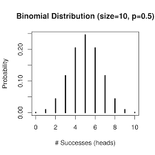
Another way to model this situation is $n$ Bernoulli trials with variable probabilities $p_{i}$ for success $X_{i}=1$ and $1-p_{i}=q_{i}$ for failure $X_{i}=0$ on the $i$ th trial where the expectations are $E\left(X_{i}\right)=p_{i}$ and those probabilities make up a distribution, i.e., $\sum_{i=1}^{n} p_{i}=1$. The random variable for the number of successes is: $S=\sum_{i=1}^{n} X_{i}$ with the expectation $E(S)=\sum_{i} E\left(X_{i}\right)=\sum_{i} p_{i}=1$. The variance of $X_{i}$ is:
$$
\begin{aligned}
\operatorname{Var}\left(X_{i}\right) &=E\left[\left(X_{i}-p_{i}\right)\left(X_{i}-p_{i}\right)\right]=\left(1-p_{i}\right)^{2} p_{i}+\left(0-p_{i}\right)^{2} q_{i} \
&=q_{i}^{2} p_{i}+p_{i}^{2} q_{i}=p_{i} q_{i}\left(p_{i}+q_{i}\right)=p_{i}\left(1-p_{i}\right)
\end{aligned}
$$
数学代写|信息论代写information theory代考|Boltzmann and Shannon Entropies
In Boltzmannian statistical mechanics, when $n$ particles can be in $m$ different distinguishable “states” (e.g., levels of energy), then a configuration or macrostate $\left(n_{1}, \ldots, n_{m}\right)$ is given by the occupation numbers $n_{i}$ of particles in the $i$ th state where $n_{1}+\ldots+n_{m}=n$. Then the total number of possible microstates for that configuration is the multinomial coefficient $\left(\begin{array}{c}n \ n_{1}, \ldots, n_{m}\end{array}\right)=\frac{n !}{n_{1} ! \ldots n_{m} !}$. If all the $m^{n}$ possible states are equiprobable, then the larger the multinomial coefficient, the higher probability that a system will be in that state. The system will spontaneously propagate to higher probability states subject to the constraint that the sum of the energies of the particles is a constant, the total energy in the system. Hence to find the characteristics of the equilibrium towards which a system will spontaneously evolve, one needs to maximize the multinomial coefficient subject to the energy constraint. The natural logarithm of the multinomial coefficient is a monotonic transformation so maximizing the one is equivalent to maximizing the other. And taking the natural log of the multinomial coefficient yields an additive quantity to be associated with the extensive quantity of entropy in thermodynamics.
The Boltzmann entropy ${ }^{5} \ln \left(\frac{n !}{n_{1} ! \ldots n_{m} !}\right)$ is usually represented as related to the Shannon entropy via the two-term Stirling approximation. It is important to note that the Boltzmann entropy is already a Shannon entropy for the probability distribution of $p=\left(1 / \frac{n !}{n_{1} ! \ldots n_{m} !}, \ldots, 1 / \frac{n !}{n_{1} ! \ldots n_{m} !}\right)$ where all the microstates for the configuration $\left(n_{1}, \ldots, n_{m}\right)$ are equiprobable:
$$
\begin{gathered}
H_{e}\left(1 / \frac{n !}{n_{1} ! \ldots n_{m} !}, \ldots, 1 / \frac{n !}{n_{1} ! \ldots n_{m} !}\right)=\sum_{i=1}^{\frac{n !}{n_{1} \cdots n_{m}}} \frac{1}{\frac{n !}{n ! ! \ldots n_{m} !}} \ln \left(\frac{1}{1 / \frac{n !}{n_{1} ! \ldots n_{m} !}}\right) \
\quad=\frac{n !}{n_{1} ! \ldots n_{m} !} \frac{1}{\frac{n !}{n ! \ldots n_{m} !}} \ln \left(\frac{n !}{n_{1} ! \ldots n_{m} !}\right)=\ln \left(\frac{n !}{n_{1} ! \ldots n_{m} !}\right)
\end{gathered}
$$
There is no approximation involved. Taking the Shannon entropy to base 2 , the usual interpretation is that it is the average number of yes-or-no questions it takes to determine the specific microstate given the macrostate. The logical entropy for that probability distribution is: $h\left(1 / \frac{n !}{n_{1} ! \ldots n_{m} !}, \ldots, 1 / \frac{n !}{n_{1} ! \ldots n_{m} !}\right)=1-\frac{1}{\frac{n !}{n_{1} ! \ldots n_{m} !}}$
数学代写|信息论代写information theory代考|MaxEntropies for Discrete Distributions
Given a function $X: U \rightarrow \mathbb{R}$ with metrical real values $\left(x_{1}, \ldots, x_{n}\right)$, what is the probability distribution $p=\left(p_{1}, \ldots, p_{n}\right)$ such that $\sum_{i=1}^{n} p_{i} x_{i}=m$ for a given mean or average $m$ such that logical entropy is a maximum? Since there are inequality constraints $p_{i} \geq 0$ on the variables and since logical entropy is quadratic in the variables, this is a quadratic programming problem. But we can first approach it as a classical optimization problem (equality constraints and no non-negativity constraints on the variables) and then derive the conditions on $m$ so that all the probabilities will be non-negative anyway.
The Lagrangian for the maximization problem is:
$$
\mathcal{L}\left(p_{1}, \ldots, p_{n}\right)=1-\sum_{i} p_{i}^{2}-\lambda\left(1-\sum p_{i}\right)+\tau\left(m-\sum p_{i} x_{i}\right)
$$
so the first-order conditions are:
$$
\partial \mathcal{L} / \partial p_{j}=-2 p_{j}+\lambda-\tau x_{j}=0 \text { so } p_{j}=\frac{1}{2}\left(\lambda-\tau x_{j}\right) .
$$
The calculations are simplified if we define $\mu=\sum_{i} x_{i} / n$ and $\operatorname{Var}(X)=E\left(X^{2}\right)-$ $\mu^{2}=\sum_{i} x_{i}^{2} / n-\mu^{2}=\sigma^{2}$. Using the first constraint:
$$
1=\sum p_{i}=\frac{1}{2}(n \lambda-\tau n \mu)=\frac{n}{2}(\lambda-\tau \mu),
$$
and using the second constraint:
$$
\begin{gathered}
m=\sum p_{i} x_{i}=\sum_{i} x_{i} \frac{1}{2}\left(\lambda-\tau x_{i}\right)=\lambda \frac{n}{2} \mu-\tau \frac{1}{2} \sum x_{i}^{2} \
=\frac{n}{2} \lambda \mu-\frac{n}{2} \tau\left[\operatorname{Var}(X)+\mu^{2}\right]=\mu\left(\frac{n}{2}(\lambda-\tau \mu)\right)-\frac{n}{2} \operatorname{Var}(X) \tau=\mu-\frac{n}{2} \operatorname{Var}(X) \tau
\end{gathered}
$$
so we have two equations that can be used to solve for the Lagrange multipliers $\lambda$ and $\tau$. Solving for $\tau$ in the second constraint:
$$
\tau=\frac{2}{n} \frac{(\mu-m)}{\operatorname{Var}(X)}
$$
信息论代考
数学代写|信息论代写information theory代考|Metrical Logical Entropy = (Twice) Variance
由于逻辑熵是对区别、差异、可区分性和多样性或异质性的度量,因此应该与统计中的方差概念相关。给定一个概率分布p=(p1,…,pn), 逻辑熵是得到不同索引的两次抽取概率H(p)=∑一世≠jp一世pj=1− ∑一世p一世2. 概率通常由随机变量的逆图像提供X:在→R在结果集或样本空间上在其中可能的值X1,…,Xn有概率p一世=公关(X=X一世)为了一世=1,…,n. 如果被建模的统计数据是分类的,那么不同的数字X一世分配给不同的类别没有度量意义,因此不能有意义地相加或相乘。但是仍然可以通过使用随机向量对情况进行建模以计算方差X=(X1,…,Xn)在每次试验中,其中一个随机变量的值为 1,其余的为 0,概率为公关(X一世=1)=p一世为了一世=1,…,n. 那么随机向量的期望是和(X)=(p1,…,pn). 向量分量上的方差为:
曾是(X)=∑一世p一世[(1−p一世)2+∑j≠一世(0−pj)2] =∑一世p一世[1−2p一世+p一世2+∑j≠一世(0−pj)2] =∑一世p一世[1−2p一世+∑jpj2] =1−2∑一世p一世2+∑jpj2=1−∑一世p一世2=H(p)
分类数据的随机向量的方差=逻辑熵。[8]
模拟这种情况的另一种方法是n具有可变概率的伯努利试验p一世为了成功X一世=1和1−p一世=q一世对于失败X一世=0在一世期望值的试验和(X一世)=p一世并且这些概率构成了一个分布,即∑一世=1np一世=1. 成功次数的随机变量是:小号=∑一世=1nX一世带着期待和(小号)=∑一世和(X一世)=∑一世p一世=1. 的方差X一世是:
曾是(X一世)=和[(X一世−p一世)(X一世−p一世)]=(1−p一世)2p一世+(0−p一世)2q一世 =q一世2p一世+p一世2q一世=p一世q一世(p一世+q一世)=p一世(1−p一世)
数学代写|信息论代写information theory代考|Boltzmann and Shannon Entropies
在玻尔兹曼统计力学中,当n粒子可以在米不同的可区分“状态”(例如,能量水平),然后是配置或宏观状态(n1,…,n米)由职业编号给出n一世中的粒子一世状态n1+…+n米=n. 那么该配置的可能微观状态的总数是多项式系数(n n1,…,n米)=n!n1!…n米!. 如果所有的米n可能的状态是等概率的,则多项式系数越大,系统处于该状态的概率就越高。系统将自发传播到更高概率的状态,受制于粒子能量之和是一个常数,即系统中的总能量。因此,要找到系统自发演化的平衡特征,需要在能量约束下最大化多项式系数。多项式系数的自然对数是单调变换,因此最大化一个等于最大化另一个。并且取多项式系数的自然对数会产生一个与热力学中熵的广泛量相关的附加量。
玻尔兹曼熵5ln(n!n1!…n米!)通常通过两项斯特林近似表示为与香农熵有关。重要的是要注意玻尔兹曼熵已经是香农熵的概率分布p=(1/n!n1!…n米!,…,1/n!n1!…n米!)配置的所有微观状态(n1,…,n米)是等概率的:
H和(1/n!n1!…n米!,…,1/n!n1!…n米!)=∑一世=1n!n1⋯n米1n!n!!…n米!ln(11/n!n1!…n米!) =n!n1!…n米!1n!n!…n米!ln(n!n1!…n米!)=ln(n!n1!…n米!)
不涉及近似值。以香农熵为底 2 ,通常的解释是它是确定宏观状态下特定微观状态所需的是或否问题的平均数量。该概率分布的逻辑熵是:H(1/n!n1!…n米!,…,1/n!n1!…n米!)=1−1n!n1!…n米!
数学代写|信息论代写information theory代考|MaxEntropies for Discrete Distributions
给定一个函数X:在→R具有度量实值(X1,…,Xn), 什么是概率分布p=(p1,…,pn)这样∑一世=1np一世X一世=米对于给定的平均值或平均值米这样逻辑熵是最大值?由于存在不等式约束p一世≥0在变量上并且由于逻辑熵在变量中是二次的,这是一个二次规划问题。但我们可以首先将其视为经典优化问题(等式约束且对变量没有非负性约束),然后推导出条件米这样所有的概率无论如何都是非负的。
最大化问题的拉格朗日是:
大号(p1,…,pn)=1−∑一世p一世2−λ(1−∑p一世)+τ(米−∑p一世X一世)
所以一阶条件是:
∂大号/∂pj=−2pj+λ−τXj=0 所以 pj=12(λ−τXj).
如果我们定义,计算会被简化μ=∑一世X一世/n和曾是(X)=和(X2)− μ2=∑一世X一世2/n−μ2=σ2. 使用第一个约束:
1=∑p一世=12(nλ−τnμ)=n2(λ−τμ),
并使用第二个约束:
米=∑p一世X一世=∑一世X一世12(λ−τX一世)=λn2μ−τ12∑X一世2 =n2λμ−n2τ[曾是(X)+μ2]=μ(n2(λ−τμ))−n2曾是(X)τ=μ−n2曾是(X)τ
所以我们有两个方程可以用来求解拉格朗日乘数λ和τ. 解决τ在第二个约束中:
τ=2n(μ−米)曾是(X)

统计代写请认准statistics-lab™. statistics-lab™为您的留学生涯保驾护航。
金融工程代写
金融工程是使用数学技术来解决金融问题。金融工程使用计算机科学、统计学、经济学和应用数学领域的工具和知识来解决当前的金融问题,以及设计新的和创新的金融产品。
非参数统计代写
非参数统计指的是一种统计方法,其中不假设数据来自于由少数参数决定的规定模型;这种模型的例子包括正态分布模型和线性回归模型。
广义线性模型代考
广义线性模型(GLM)归属统计学领域,是一种应用灵活的线性回归模型。该模型允许因变量的偏差分布有除了正态分布之外的其它分布。
术语 广义线性模型(GLM)通常是指给定连续和/或分类预测因素的连续响应变量的常规线性回归模型。它包括多元线性回归,以及方差分析和方差分析(仅含固定效应)。
有限元方法代写
有限元方法(FEM)是一种流行的方法,用于数值解决工程和数学建模中出现的微分方程。典型的问题领域包括结构分析、传热、流体流动、质量运输和电磁势等传统领域。
有限元是一种通用的数值方法,用于解决两个或三个空间变量的偏微分方程(即一些边界值问题)。为了解决一个问题,有限元将一个大系统细分为更小、更简单的部分,称为有限元。这是通过在空间维度上的特定空间离散化来实现的,它是通过构建对象的网格来实现的:用于求解的数值域,它有有限数量的点。边界值问题的有限元方法表述最终导致一个代数方程组。该方法在域上对未知函数进行逼近。[1] 然后将模拟这些有限元的简单方程组合成一个更大的方程系统,以模拟整个问题。然后,有限元通过变化微积分使相关的误差函数最小化来逼近一个解决方案。
tatistics-lab作为专业的留学生服务机构,多年来已为美国、英国、加拿大、澳洲等留学热门地的学生提供专业的学术服务,包括但不限于Essay代写,Assignment代写,Dissertation代写,Report代写,小组作业代写,Proposal代写,Paper代写,Presentation代写,计算机作业代写,论文修改和润色,网课代做,exam代考等等。写作范围涵盖高中,本科,研究生等海外留学全阶段,辐射金融,经济学,会计学,审计学,管理学等全球99%专业科目。写作团队既有专业英语母语作者,也有海外名校硕博留学生,每位写作老师都拥有过硬的语言能力,专业的学科背景和学术写作经验。我们承诺100%原创,100%专业,100%准时,100%满意。
随机分析代写
随机微积分是数学的一个分支,对随机过程进行操作。它允许为随机过程的积分定义一个关于随机过程的一致的积分理论。这个领域是由日本数学家伊藤清在第二次世界大战期间创建并开始的。
时间序列分析代写
随机过程,是依赖于参数的一组随机变量的全体,参数通常是时间。 随机变量是随机现象的数量表现,其时间序列是一组按照时间发生先后顺序进行排列的数据点序列。通常一组时间序列的时间间隔为一恒定值(如1秒,5分钟,12小时,7天,1年),因此时间序列可以作为离散时间数据进行分析处理。研究时间序列数据的意义在于现实中,往往需要研究某个事物其随时间发展变化的规律。这就需要通过研究该事物过去发展的历史记录,以得到其自身发展的规律。
回归分析代写
多元回归分析渐进(Multiple Regression Analysis Asymptotics)属于计量经济学领域,主要是一种数学上的统计分析方法,可以分析复杂情况下各影响因素的数学关系,在自然科学、社会和经济学等多个领域内应用广泛。
MATLAB代写
MATLAB 是一种用于技术计算的高性能语言。它将计算、可视化和编程集成在一个易于使用的环境中,其中问题和解决方案以熟悉的数学符号表示。典型用途包括:数学和计算算法开发建模、仿真和原型制作数据分析、探索和可视化科学和工程图形应用程序开发,包括图形用户界面构建MATLAB 是一个交互式系统,其基本数据元素是一个不需要维度的数组。这使您可以解决许多技术计算问题,尤其是那些具有矩阵和向量公式的问题,而只需用 C 或 Fortran 等标量非交互式语言编写程序所需的时间的一小部分。MATLAB 名称代表矩阵实验室。MATLAB 最初的编写目的是提供对由 LINPACK 和 EISPACK 项目开发的矩阵软件的轻松访问,这两个项目共同代表了矩阵计算软件的最新技术。MATLAB 经过多年的发展,得到了许多用户的投入。在大学环境中,它是数学、工程和科学入门和高级课程的标准教学工具。在工业领域,MATLAB 是高效研究、开发和分析的首选工具。MATLAB 具有一系列称为工具箱的特定于应用程序的解决方案。对于大多数 MATLAB 用户来说非常重要,工具箱允许您学习和应用专业技术。工具箱是 MATLAB 函数(M 文件)的综合集合,可扩展 MATLAB 环境以解决特定类别的问题。可用工具箱的领域包括信号处理、控制系统、神经网络、模糊逻辑、小波、仿真等。