如果你也在 怎样代写Generalized linear model这个学科遇到相关的难题,请随时右上角联系我们的24/7代写客服。
广义线性模型(GLiM,或GLM)是John Nelder和Robert Wedderburn在1972年提出的一种高级统计建模技术。它是一个包括许多其他模型的总称,它允许响应变量y具有正态分布以外的误差分布。
statistics-lab™ 为您的留学生涯保驾护航 在代写Generalized linear model方面已经树立了自己的口碑, 保证靠谱, 高质且原创的统计Statistics代写服务。我们的专家在代写Generalized linear model代写方面经验极为丰富,各种代写Generalized linear model相关的作业也就用不着说。
我们提供的Generalized linear model及其相关学科的代写,服务范围广, 其中包括但不限于:
- Statistical Inference 统计推断
- Statistical Computing 统计计算
- Advanced Probability Theory 高等概率论
- Advanced Mathematical Statistics 高等数理统计学
- (Generalized) Linear Models 广义线性模型
- Statistical Machine Learning 统计机器学习
- Longitudinal Data Analysis 纵向数据分析
- Foundations of Data Science 数据科学基础
统计代写|Generalized linear model代考广义线性模型代写|Frequency Tables
One of the simplest ways to display data is in a frequency table. To create a frequency table for a variable, you need to list every value for the variable in the dataset and then list the frequency, which is the count of how many times each value occurs. Table 3.2a shows an example from Waite et al.’s (2015) study. When asked how much the subjects agree with the statement “I feel that my sibling understands me well,” one person strongly disagreed, three people disagreed, three felt neutral about the statement, five agreed, and one strongly agreed. A frequency table just compiles this information in an easy to use format, as shown below. The first column of a frequency table consists of the response label (labeled “Response”) and the second column is the number of each response (labeled “Frequency”).
Frequency tables can only show data for one variable at a time, but they are helpful for discerning general patterns within a variable. Table $3.2 \mathrm{a}$, for example, shows that few people in the Waite et al. (2015) study felt strongly about whether their sibling with autism understood them well. Most responses clustered towards the middle of the scale.
Table $3.2 \mathrm{a}$ also shows an important characteristic of frequency tables: the number of responses adds up to the number of participants in the study. This will be true if there are responses from everyone in the study (as is the case in Waite et al.’s study).
Frequency tables can include additional information about subjects’ scores in new columns. The first new column is labeled “Cumulative frequency,” which is determined by counting the number of people in a row and adding it to the number of people in higher rows in the frequency table. For example, in Table $3.2 \mathrm{~b}$, the cumulative frequency for the second row (labeled “Disagree”) is 4 – which was calculated by summing the frequency from that row, which was 3 , and the
frequency of the higher row, which was $1(3+1=4)$. As another example, the cumulative frequency column shows that, for example, 7 of the 13 respondents responded “strongly disagree,” “disagree,” or “neutral” when asked about whether their sibling with autism understood them well.
It is also possible to use a frequency table to identify the proportion of people giving each response. In a frequency table, a proportion is a number expressed as a decimal or a fraction that shows how many subjects in the dataset have the same value for a variable. To calculate the proportion of people who gave each response, use the following formula:
$$
\text { Proportion }=\frac{f}{n} \quad \text { (Formula 3.1) }
$$
In Formula $3.1, f$ is the frequency of a response, and $n$ is the sample size. Therefore, calculating the proportion merely requires finding the frequency of a response and dividing it by the number of people in the sample. Proportions will always be between the values of 0 to 1 .
Table $3.3$ shows the frequency table for the Waite et al. (2015) study, with new columns showing the proportions for the frequencies and the cumulative frequencies. The table nicely provides examples of the properties of proportions. For example, it is apparent that all of the values in both the “Frequency proportion” and “Cumulative proportion” columns are between 0 and 1.0. Additionally, those columns show how the frequency proportions were calculated – by taking the number in the frequency column and dividing by $n$ (which is 13 in this small study). A similar process was used to calculate the cumulative proportions in the far right column.
Table $3.3$ is helpful in visualizing data because it shows quickly which variable responses were most common and which responses were rare. It is obvious, for example, that “Agree” was the most common response to the question of whether the subjects’ sibling with autism understood them well, which is apparent because that response had the highest frequency (5) and the highest frequency proportion (.385). Likewise, “strongly disagree” and “strongly agree” were unusual responses because they tied for having the lowest frequency (1) and lowest frequency proportion (.077). Combined together, this information reveals that even though autism is characterized by pervasive difficulties in social situations and interpersonal relationships, many people with autism can still have a relationship with their sibling without a disability (Waite et al., 2015). This is important information for professionals who work with families that include a person with a diagnosis of autism.
统计代写|Generalized linear model代考广义线性模型代写|Histograms
Frequency tables are very helpful, but they have a major drawback: they are just a summary of the data, and they are not very visual. For people who prefer a picture to a table, there is the option of creating a histogram, an example of which is shown below in Figure 3.1.
A histogram converts the data in a frequency table into visual format. Each bar in a histogram (called an interval) represents a range of possible values for a variable. The height of the bar represents the frequency of responses within the range of the interval. In Figure $3.1$ it is clear that, for the second bar, which represents the “disagree” response, three people gave this response (because the bar is 3 units high).
Notice how the variable scores (i.e., 1, 2, 3, 4, or 5) are in the middle of the interval for each bar. Technically, this means that the interval includes more than just whole number values. This is illustrated in Figure 3.2, which shows that each interval has a width of 1 unit. The figure also annotates how, for the second bar, the interval ranges between $1.5$ and $2.5$. In Waite et al.’s study (2015), all of the responses were whole numbers, but this is not always true of social science data, especially for variables that can be measured very precisely, such as reaction time (often measured in milliseconds) or grade-point average (often calculated to two or three decimal places).
Figures $3.1$ and $3.2$ also show another important characteristic of histograms: the bars in the histogram touch. This is because the variable on this histogram is assumed to measure a continuous trait (i.e., level of agreement), even if Waite et al. (2015) only permitted their subjects to give five possible responses to the question. In other words, there are probably subtle differences in how much each subject agreed with the statement that their sibling with autism knows them well. If Waite et al. (2015) had a more precise way of measuring their subjects’ responses, it is possible that the data would include responses that were not whole numbers, such as $1.8,2.1$, and 2.3. However, if only whole numbers were permitted in their data, these responses would be rounded to 2. Yet, it is still possible that there are differences in the subjects’ actual levels of agreement. Having the histogram bars touch shows that, theoretically, the respondents’ opinions are on a continuum.
The only gaps in a histogram should occur in intervals where there are no values for a variable within the interval. An example of the types of gaps that are appropriate for a histogram is Figure $3.3$, which is a histogram of the subjects’ ages.
The gaps in Figure $3.3$ are acceptable because they represent intervals where there were no subjects. For example, there were no subjects in the study who were 32 years old. (This can be verified by checking Table 3.1, which shows the subjects’ ages in the third column.) Therefore, there is a gap at this place on the histogram in Figure 3.3.
Some people do not like having a large number of intervals in their histograms, so they will combine intervals as they build their histogram. For example, having intervals that span 3 years instead of 1 year will change Figure $3.3$ into Figure 3.4.
Combining intervals simplifies the visual model even more, but this simplification may be needed. In some studies with precisely measured variables or large sample sizes, having an interval for every single value of a variable may result in complex histograms that are difficult to understand. By simplifying the visual model, the data become more intelligible. There are no firm guidelines for choosing the number of intervals in a histogram, but I recommend having no fewer than five. Regardless of the number of intervals you choose for a histogram, you should always ensure that the intervals are all the same width.
统计代写|Generalized linear model代考广义线性模型代写|Number of Peaks
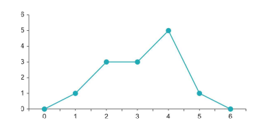
Another way to describe distributions is to describe the number of peaks that the histogram has. A distribution with a single peak is called a unimodal distribution. All of the distributions in the chapter so far (including the normal distribution in Figure $3.9$ and Quetelet’s data in Figure $3.10$ ) are unimodal distributions because they have one peak. The term “-modal” refers to the most common score in a distribution, a concept explained in further detail in Chapter $4 .$
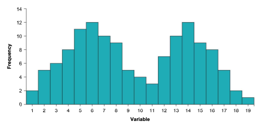
Sometimes distributions have two peaks, as in Figure 3.17. When a distribution has two peaks, it is called a bimodal distribution. In the social sciences most distributions have only one peak, but bimodal distributions like the one in Figure $3.17$ occur occasionally, as in Lacritz et al.’s (2004) study that found that people’s test scores on a test of visual short-term memory were bimodal. In that case the peaks of the histograms were at the two extreme ends of the distribution – meaning people tended to have very poor or very good recognition of pictures they had seen earlier. Bimodal distributions can occur when a sample consists of two different groups (as when some members of a sample have had a treatment and the other sample members have not).
广义线性模型代写
统计代写|Generalized linear model代考广义线性模型代写|Frequency Tables
显示数据的最简单方法之一是在频率表中。要为变量创建频率表,您需要列出数据集中变量的每个值,然后列出频率,即每个值出现次数的计数。表 3.2a 显示了 Waite 等人 (2015) 研究的一个示例。当被问及受试者对“我觉得我的兄弟姐妹很了解我”这句话的同意程度时,一个人非常不同意,三个人不同意,三个人对这个陈述持中立态度,五个人同意,一个人非常同意。频率表只是以易于使用的格式编译此信息,如下所示。频率表的第一列由响应标签(标记为“响应”)组成,第二列是每个响应的数量(标记为“频率”)。
频率表一次只能显示一个变量的数据,但它们有助于识别变量中的一般模式。桌子3.2一种,例如,表明在 Waite 等人中很少有人。(2015)的研究强烈认为他们的自闭症兄弟姐妹是否理解他们。大多数反应集中在量表的中间。
桌子3.2一种还显示了频率表的一个重要特征:响应的数量加起来就是研究参与者的数量。如果研究中的每个人都有回应,这将是正确的(就像 Waite 等人的研究中的情况一样)。
频率表可以在新列中包含有关科目分数的附加信息。第一个新列标记为“累积频率”,它是通过计算一行中的人数并将其添加到频率表中较高行的人数来确定的。例如,在表3.2 b,第二行(标记为“不同意”)的累积频率为 4 – 这是通过将该行的频率相加计算得出的,即 3 ,并且
较高行的频率,即1(3+1=4). 作为另一个例子,累积频率列显示,例如,当被问及自闭症兄弟姐妹是否理解他们时,13 名受访者中有 7 人回答“非常不同意”、“不同意”或“中立”。
也可以使用频率表来确定给出每个响应的人的比例。在频率表中,比例是表示为小数或分数的数字,显示数据集中有多少受试者具有相同的变量值。要计算给出每个响应的人的比例,请使用以下公式:
部分 =Fn (公式 3.1)
在公式中3.1,F是响应的频率,并且n是样本量。因此,计算比例只需要找到响应的频率并将其除以样本中的人数。比例将始终介于 0 到 1 的值之间。
桌子3.3显示了 Waite 等人的频率表。(2015) 研究,新列显示频率和累积频率的比例。该表很好地提供了比例属性的示例。例如,很明显“频率比例”和“累积比例”列中的所有值都在 0 和 1.0 之间。此外,这些列显示了频率比例的计算方式——通过将频率列中的数字除以n(在这个小型研究中是 13)。使用类似的过程来计算最右列中的累积比例。
桌子3.3有助于可视化数据,因为它可以快速显示哪些变量响应最常见,哪些响应很少。很明显,例如,对于受试者的自闭症兄弟姐妹是否理解他们的问题,“同意”是最常见的回答,这很明显,因为该回答具有最高频率(5)和最高频率比例( .385)。同样,“非常不同意”和“非常同意”是不寻常的反应,因为它们具有最低频率 (1) 和最低频率比例 (0.077)。综合起来,这些信息表明,尽管自闭症的特点是在社交场合和人际关系中普遍存在困难,但许多自闭症患者仍然可以与没有残疾的兄弟姐妹建立关系(Waite 等,2015)。
统计代写|Generalized linear model代考广义线性模型代写|Histograms
频率表非常有用,但它们有一个主要缺点:它们只是数据的摘要,并且不是很直观。对于喜欢图片而不是表格的人,可以选择创建直方图,图 3.1 中显示了一个示例。
直方图将频率表中的数据转换为可视格式。直方图中的每个条形(称为区间)代表变量可能值的范围。条形的高度表示区间范围内的响应频率。如图3.1很明显,对于代表“不同意”响应的第二个条形,三个人给出了这个响应(因为条形高 3 个单位)。
请注意变量分数(即 1、2、3、4 或 5)如何位于每个条的区间中间。从技术上讲,这意味着区间不仅包括整数值。图 3.2 对此进行了说明,该图显示每个间隔的宽度为 1 个单位。该图还注释了第二个条的间隔范围1.5和2.5. 在 Waite 等人的研究(2015 年)中,所有响应都是整数,但社会科学数据并非总是如此,特别是对于可以非常精确测量的变量,例如反应时间(通常以毫秒为单位) ) 或平均成绩(通常计算到小数点后两位或三位)。
数据3.1和3.2还显示了直方图的另一个重要特征:直方图中的条形触摸。这是因为假设该直方图上的变量衡量的是连续性状(即一致性水平),即使 Waite 等人也如此。(2015)只允许他们的受试者对这个问题给出五种可能的回答。换句话说,每个受试者在多大程度上同意他们的自闭症兄弟姐妹非常了解他们的说法可能存在细微的差异。如果韦特等人。(2015)有一种更精确的方法来衡量他们的受试者的反应,数据可能包括不是整数的反应,例如1.8,2.1,和 2.3。但是,如果他们的数据中只允许整数,则这些响应将四舍五入为 2。然而,受试者的实际一致性水平仍然可能存在差异。让直方图条形接触表明,理论上,受访者的意见是连续的。
直方图中唯一的间隙应该出现在区间内没有变量值的区间内。适合直方图的间隙类型示例如下图3.3,这是受试者年龄的直方图。
图中的差距3.3是可以接受的,因为它们代表没有主题的区间。例如,研究中没有 32 岁的受试者。(这可以通过查看表 3.1 来验证,表 3.1 在第三列中显示了受试者的年龄。)因此,在图 3.3 的直方图上这个地方有一个差距。
有些人不喜欢在他们的直方图中有大量的区间,所以他们会在构建直方图时组合区间。例如,间隔 3 年而不是 1 年将改变图3.3进入图 3.4。
组合区间进一步简化了视觉模型,但可能需要这种简化。在一些具有精确测量变量或大样本量的研究中,为变量的每个单个值设置一个区间可能会导致难以理解的复杂直方图。通过简化可视化模型,数据变得更易理解。在直方图中选择区间数没有明确的指导方针,但我建议不少于五个。无论您为直方图选择多少间隔,您都应始终确保所有间隔的宽度相同。
统计代写|Generalized linear model代考广义线性模型代写|Number of Peaks
描述分布的另一种方法是描述直方图的峰值数量。具有单峰的分布称为单峰分布。到目前为止本章中的所有分布(包括图中的正态分布)3.9和Quetelet的数据如图3.10) 是单峰分布,因为它们有一个峰值。术语“-modal”指的是分布中最常见的分数,这一概念在第 1 章中有更详细的解释4.
有时分布有两个峰值,如图 3.17 所示。当一个分布有两个峰时,称为双峰分布。在社会科学中,大多数分布只有一个峰值,但是如图中所示的双峰分布3.17偶尔会发生,如 Lacritz 等人 (2004) 的研究发现,人们在视觉短期记忆测试中的测试分数是双峰的。在这种情况下,直方图的峰值位于分布的两个极端——这意味着人们对他们之前看到的图片的识别往往很差或很好。当样本由两个不同的组组成时(如样本中的一些成员接受过治疗而其他样本成员没有接受过治疗),就会出现双峰分布。

统计代写请认准statistics-lab™. statistics-lab™为您的留学生涯保驾护航。
金融工程代写
金融工程是使用数学技术来解决金融问题。金融工程使用计算机科学、统计学、经济学和应用数学领域的工具和知识来解决当前的金融问题,以及设计新的和创新的金融产品。
非参数统计代写
非参数统计指的是一种统计方法,其中不假设数据来自于由少数参数决定的规定模型;这种模型的例子包括正态分布模型和线性回归模型。
广义线性模型代考
广义线性模型(GLM)归属统计学领域,是一种应用灵活的线性回归模型。该模型允许因变量的偏差分布有除了正态分布之外的其它分布。
术语 广义线性模型(GLM)通常是指给定连续和/或分类预测因素的连续响应变量的常规线性回归模型。它包括多元线性回归,以及方差分析和方差分析(仅含固定效应)。
有限元方法代写
有限元方法(FEM)是一种流行的方法,用于数值解决工程和数学建模中出现的微分方程。典型的问题领域包括结构分析、传热、流体流动、质量运输和电磁势等传统领域。
有限元是一种通用的数值方法,用于解决两个或三个空间变量的偏微分方程(即一些边界值问题)。为了解决一个问题,有限元将一个大系统细分为更小、更简单的部分,称为有限元。这是通过在空间维度上的特定空间离散化来实现的,它是通过构建对象的网格来实现的:用于求解的数值域,它有有限数量的点。边界值问题的有限元方法表述最终导致一个代数方程组。该方法在域上对未知函数进行逼近。[1] 然后将模拟这些有限元的简单方程组合成一个更大的方程系统,以模拟整个问题。然后,有限元通过变化微积分使相关的误差函数最小化来逼近一个解决方案。
tatistics-lab作为专业的留学生服务机构,多年来已为美国、英国、加拿大、澳洲等留学热门地的学生提供专业的学术服务,包括但不限于Essay代写,Assignment代写,Dissertation代写,Report代写,小组作业代写,Proposal代写,Paper代写,Presentation代写,计算机作业代写,论文修改和润色,网课代做,exam代考等等。写作范围涵盖高中,本科,研究生等海外留学全阶段,辐射金融,经济学,会计学,审计学,管理学等全球99%专业科目。写作团队既有专业英语母语作者,也有海外名校硕博留学生,每位写作老师都拥有过硬的语言能力,专业的学科背景和学术写作经验。我们承诺100%原创,100%专业,100%准时,100%满意。
随机分析代写
随机微积分是数学的一个分支,对随机过程进行操作。它允许为随机过程的积分定义一个关于随机过程的一致的积分理论。这个领域是由日本数学家伊藤清在第二次世界大战期间创建并开始的。
时间序列分析代写
随机过程,是依赖于参数的一组随机变量的全体,参数通常是时间。 随机变量是随机现象的数量表现,其时间序列是一组按照时间发生先后顺序进行排列的数据点序列。通常一组时间序列的时间间隔为一恒定值(如1秒,5分钟,12小时,7天,1年),因此时间序列可以作为离散时间数据进行分析处理。研究时间序列数据的意义在于现实中,往往需要研究某个事物其随时间发展变化的规律。这就需要通过研究该事物过去发展的历史记录,以得到其自身发展的规律。
回归分析代写
多元回归分析渐进(Multiple Regression Analysis Asymptotics)属于计量经济学领域,主要是一种数学上的统计分析方法,可以分析复杂情况下各影响因素的数学关系,在自然科学、社会和经济学等多个领域内应用广泛。
MATLAB代写
MATLAB 是一种用于技术计算的高性能语言。它将计算、可视化和编程集成在一个易于使用的环境中,其中问题和解决方案以熟悉的数学符号表示。典型用途包括:数学和计算算法开发建模、仿真和原型制作数据分析、探索和可视化科学和工程图形应用程序开发,包括图形用户界面构建MATLAB 是一个交互式系统,其基本数据元素是一个不需要维度的数组。这使您可以解决许多技术计算问题,尤其是那些具有矩阵和向量公式的问题,而只需用 C 或 Fortran 等标量非交互式语言编写程序所需的时间的一小部分。MATLAB 名称代表矩阵实验室。MATLAB 最初的编写目的是提供对由 LINPACK 和 EISPACK 项目开发的矩阵软件的轻松访问,这两个项目共同代表了矩阵计算软件的最新技术。MATLAB 经过多年的发展,得到了许多用户的投入。在大学环境中,它是数学、工程和科学入门和高级课程的标准教学工具。在工业领域,MATLAB 是高效研究、开发和分析的首选工具。MATLAB 具有一系列称为工具箱的特定于应用程序的解决方案。对于大多数 MATLAB 用户来说非常重要,工具箱允许您学习和应用专业技术。工具箱是 MATLAB 函数(M 文件)的综合集合,可扩展 MATLAB 环境以解决特定类别的问题。可用工具箱的领域包括信号处理、控制系统、神经网络、模糊逻辑、小波、仿真等。