如果你也在 怎样代写复变函数Complex function这个学科遇到相关的难题,请随时右上角联系我们的24/7代写客服。
复数函数是一个从复数到复数的函数。换句话说,它是一个以复数的一个子集为域,以复数为子域的函数。复数函数通常应该有一个包含复数平面的非空开放子集的域。
statistics-lab™ 为您的留学生涯保驾护航 在代写复变函数Complex function方面已经树立了自己的口碑, 保证靠谱, 高质且原创的统计Statistics代写服务。我们的专家在代写复变函数Complex function代写方面经验极为丰富,各种代写复变函数Complex function相关的作业也就用不着说。
我们提供的复变函数Complex function及其相关学科的代写,服务范围广, 其中包括但不限于:
- Statistical Inference 统计推断
- Statistical Computing 统计计算
- Advanced Probability Theory 高等概率论
- Advanced Mathematical Statistics 高等数理统计学
- (Generalized) Linear Models 广义线性模型
- Statistical Machine Learning 统计机器学习
- Longitudinal Data Analysis 纵向数据分析
- Foundations of Data Science 数据科学基础
数学代写|复变函数作业代写Complex function代考|The Behavior of a Holomorphic Function
In the proof of the Cauchy integral formula in Section 2.4, we saw that it is often important to consider a function that is holomorphic on a punctured open set $U \backslash{P} \subset \mathbb{C}$. The consideration of a holomorphic function with such an “isolated singularity” turns out to occupy a central position in much of the subject. These singularities can arise in various ways. Perhaps the most obvious way occurs as the reciprocal of a holomorphic function, for instance passing from $z^{j}$ to $1 / z^{j}, j$ a positive integer. More complicated examples can be generated, for instance, by exponentiating the reciprocals of holomorphic functions: for example, $e^{1 / z}, z \neq 0$.
In this chapter we shall study carefully the behavior of holomorphic functions near a singularity. In particular, we shall obtain a new kind of infinite series expansion which generalizes the idea of the power series expansion of a holomorphic function about a (nonsingular) point. We shall in the process completely classify the behavior of holomorphic functions near an isolated singular point.
Let $U \subseteq \mathbb{C}$ be an open set and $P \in U$. Suppose that $f: U \backslash{P} \rightarrow \mathbb{C}$ is holomorphic. In this situation we say that $f$ has an isolated singular point (or isolated singularity) at $P$. The implication of the phrase is usually just that $f$ is defined and holomorphic on some such “deleted neighborhood” of $P$. The specification of the set $U$ is of secondary interest; we wish to consider the behavior of $f$ “near $P^{\prime \prime}$.
There are three possibilities for the behavior of $f$ near $P$ that are worth distinguishing:
(i) $|f(z)|$ is bounded on $D(P, r) \backslash{P}$ for some $r>0$ with $D(P, r) \subseteq$ $U$; that is, there is some $r>0$ and some $M>0$ such that $|f(z)| \leq$ $M$ for all $z \in U \cap D(P, r) \backslash{P}$.
(ii) $\lim _{z \rightarrow P}|f(z)|=+\infty$.
(iii) Neither (i) nor (ii) applies.
Of course this classification does not say much unless we can find some other properties of $f$ related to (i), (ii), and (iii). We shall prove momentarily that if case (i) holds, then $f$ has a limit at $P$ which extends $f$ so that it is holomorphic on all of $U$. It is commonly said in this circumstance that $f$ has a removable singularity at $P$. In case (ii), we will say that $f$ has a pole at $P$. In case (iii), $f$ will be said to have an essential singularity at $P$. Our goal in this and the next section is to understand (i), (ii), and (iii) in some further detail.
Theorem 4.1.1 (The Riemann removable singularities theorem). Let $f$ : $D(P, r) \backslash{P} \rightarrow \mathbb{C}$ be holomorphic and bounded. Then
(1) $\lim {z \rightarrow P} f(z)$ exists; (2) the function $\widehat{f}: D(P, r) \rightarrow \mathbb{C}$ defined by $$ \widehat{f}(z)=\left{\begin{array}{lll} f(z) & \text { if } & z \neq P \ \lim {\zeta \rightarrow P} f(\zeta) & \text { if } & z=P
\end{array}\right.
$$
is holomorphic.
数学代写|复变函数作业代写Complex function代考|Expansion around Singular Points
To aid in our further understanding of poles and essential singularities, we are going to develop a method of series expansion of holomorphic functions on $D(P, r) \backslash{P}$. Except for removable singularities, we cannot expect to expand such a function in a power series convergent in a neighborhood of $P$, since such a power series would define a holomorphic function on a whole neighborhood of $P$, including $P$ itself. A natural extension of the idea of power series is to allow negative as well as positive powers of $(z-P)$. This extension turns out to be enough to handle poles and essential singularities
both. That it works well for poles is easy to see; essential singularities take a bit more work. We turn now to the details.
A Laurent series on $D(P, r)$ is a (formal) expression of the form
$$
\sum_{j=-\infty}^{+\infty} a_{j}(z-P)^{j}
$$
Note that the individual terms are each defined for all $z \in D(P, r) \backslash{P}$.
To discuss Laurent series in terms of convergence, we must first make a general agreement as to the meaning of the convergence of a “doubly infinite” series $\sum_{j=-\infty}^{+\infty} \alpha_{j}$. We say that such a series converges if $\sum_{j=0}^{+\infty} \alpha_{j}$ and $\sum_{j=1}^{+\infty} \alpha_{-j}$ converge in the usual sense. In this case, we set
$$
\sum_{-\infty}^{+\infty} \alpha_{j}=\left(\sum_{j=0}^{+\infty} \alpha_{j}\right)+\left(\sum_{j=1}^{+\infty} \alpha_{-j}\right)
$$
You can check easily that $\sum_{-\infty}^{+\infty} \alpha_{j}$ converges to a complex number $\sigma$ if and only if for each $\epsilon>0$ there is an $N>0$ such that, if $\ell \geq N$ and $k \geq N$, then $\left|\left(\sum_{j=-k}^{\ell} \alpha_{j}\right)-\sigma\right|<\epsilon$. It is important to realize that $\ell$ and $k$ are independent here. [In particular, the existence of the limit $\lim {k \rightarrow+\infty} \sum{j=-k}^{+k} \alpha_{j}$ does not imply in general that $\sum_{-\infty}^{+\infty} \alpha_{j}$ converges. See Exercises 10 and 11.]
With these convergence ideas in mind, we can now present the analogue for Laurent series of Lemmas $3.2 .3$ and $3.2 .5$ for power series.
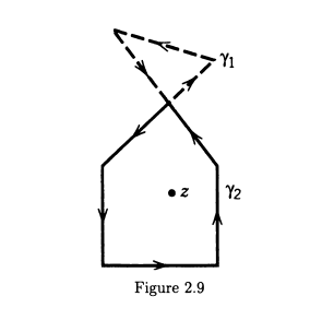
Lemma 4.2.1. If $\sum_{j=-\infty}^{+\infty} a_{j}(z-P)^{j}$ converges at $z_{1} \neq P$ and at $z_{2} \neq P$ and if $\left|z_{1}-P\right|<\left|z_{2}-P\right|$, then the series converges for all $z$ with $\left|z_{1}-P\right|<$ $|z-P|<\left|z_{2}-P\right|$.
Refer to Figure $4.1$ for an illustration of the situation described in the Lemma.
Proof of Lemma 4.2.1. If $\sum_{j=-\infty}^{+\infty} a_{j}\left(z_{2}-P\right)^{j}$ converges, then the definition of convergence of a doubly infinite sum implies that $\sum_{j=0}^{+\infty} a_{j}\left(z_{2}-P\right)^{j}$ converges. By Lemma $3.2 .3, \sum_{j=0}^{+\infty} a_{j}(z-P)^{j}$ then converges when $|z-P|<$ $\left|z_{2}-P\right|$. If $\sum_{j=-\infty}^{+\infty} a_{j}\left(z_{1}-P\right)^{j}$ converges, then so does $\sum_{j=1}^{+\infty} a_{-j}\left(z_{1}-P\right)^{-j}$. Since $0<\left|z_{1}-P\right|<|z-P|$, it follows that $|1 /(z-P)|<\left|1 /\left(z_{1}-P\right)\right|$. Hence Lemma 3.2.3 again applies to show that $\sum_{j=1}^{+\infty} a_{-j}(z-P)^{-j}$ converges. Thus $\sum_{-\infty}^{+\infty} a_{j}(z-P)^{j}$ converges when $\left|z_{1}-P\right|<|z-P|<\left|z_{2}-P\right|$.
数学代写|复变函数作业代写Complex function代考|Existence of Laurent Expansions
We turn now to establishing that convergent Laurent expansions of functions holomorphic on an annulus do in fact exist. We will require the following result.
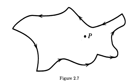
Theorem 4.3.1 (The Cauchy integral formula for an annulus). Suppose that $0 \leq r_{1}<r_{2} \leq+\infty$ and that $f: D\left(P, r_{2}\right) \backslash \bar{D}\left(P, r_{1}\right) \rightarrow \mathbb{C}$ is holomorphic. Then, for each $s_{1}, s_{2}$ such that $r_{1}<s_{1}<s_{2}<r_{2}$ and each $z \in D\left(P, s_{2}\right) \backslash$ $\bar{D}\left(P, s_{1}\right)$, it holds that
$$
f(z)=\frac{1}{2 \pi i} \oint_{|\zeta-P|=s_{2}} \frac{f(\zeta)}{\zeta-z} d \zeta-\frac{1}{2 \pi i} \oint_{|\zeta-P|=s_{1}} \frac{f(\zeta)}{\zeta-z} d \zeta .
$$
Proof. Fix a point $z \in D\left(P, s_{2}\right) \backslash \bar{D}\left(P, s_{1}\right)$. Define, for $\zeta \in D\left(P, r_{2}\right) \backslash$ $\bar{D}\left(P, r_{1}\right)$,
$$
g_{z}(\zeta)= \begin{cases}\frac{f(\zeta)-f(z)}{\zeta-z} & \zeta \neq z \ f^{\prime}(z) & \zeta=z\end{cases}
$$
Then $g_{z}$ is a holomorphic function of $\zeta, \zeta \in D\left(P, r_{2}\right) \backslash \bar{D}\left(P, r_{1}\right)$ (by the Riemann removable singularities theorem).
Now we consider the integrals
$$
\oint_{|\zeta-P|=s_{1}} g_{z}(\zeta) d \zeta
$$
and
$$
\oint_{|\zeta-P|=s_{2}} g_{z}(\zeta) d \zeta
$$
By the considerations in Section 2.6, these two. integrals are equal. So
$$
0=\oint_{|\zeta-P|=s_{2}} g_{z}(\zeta) d \zeta-\oint_{|\zeta-P|=s_{1}} g_{z}(\zeta) d \zeta
$$
$$
=\oint_{|\zeta-P|=s_{2}} \frac{f(\zeta)-f(z)}{\zeta-z} d \zeta-\oint_{|\zeta-P|=s_{1}} \frac{f(\zeta)-f(z)}{\zeta-z} d \zeta
$$
Hence
$$
\begin{aligned}
&\oint_{|\zeta-P|=s_{2}} \frac{f(\zeta)}{\zeta-z} d \zeta-\oint_{|\zeta-P|=s_{2}} \frac{f(z)}{\zeta-z} d \zeta \
&=\oint_{|\zeta-P|=s_{1}} \frac{f(\zeta)}{\zeta-z} d \zeta-\oint_{|\zeta-P|=s_{1}} \frac{f(z)}{\zeta-z} d \zeta
\end{aligned}
$$
Now
$$
\oint_{|\zeta-P|=s_{2}} \frac{f(z)}{\zeta-z} d \zeta=f(z) \oint_{|\zeta-P|=s_{2}} \frac{1}{\zeta-z} d \zeta=2 \pi i f(z)
$$
by the Cauchy integral formula for the constant function 1 on $D\left(P, r_{2}\right)$ (or by direct calculation).
Also
$$
\oint_{|\zeta-P|=s_{1}} \frac{f(z)}{\zeta-z} d \zeta=f(z) \oint_{|\zeta-P|=s_{1}} \frac{1}{\zeta-z} d \zeta=0 .
$$
This can be seen from the Cauchy integral theorem (Theorem 2.4.3) since $1 /(\zeta-z)$ is holomorphic for $\zeta \in D(P,|z-P|)$ and $\left{\zeta:|\zeta-P| \leq s_{1}\right} \subseteq$ $D(P,|z-P|)$. See Figure $4.2$.
So
$$
2 \pi i f(z)=\oint_{|\zeta-P|=s_{2}} \frac{f(\zeta)}{\zeta-z} d \zeta-\oint_{|\zeta-P|=s_{1}} \frac{f(\zeta)}{\zeta-z} d \zeta
$$
as desired.
复变函数代写
数学代写|复变函数作业代写Complex function代考|The Behavior of a Holomorphic Function
在第 2.4 节的柯西积分公式的证明中,我们看到考虑一个在穿孔开集上的全纯函数通常很重要在∖磷⊂C. 对具有这种“孤立奇点”的全纯函数的考虑在该主题的大部分内容中占据了中心位置。这些奇点可以以各种方式出现。也许最明显的方式是作为全纯函数的倒数出现,例如从和j到1/和j,j一个正整数。例如,可以通过对全纯函数的倒数求幂来生成更复杂的示例:例如,和1/和,和≠0.
在本章中,我们将仔细研究全纯函数在奇点附近的行为。特别是,我们将获得一种新的无限级数展开,它推广了关于(非奇异)点的全纯函数的幂级数展开的概念。在此过程中,我们将对孤立奇异点附近的全纯函数的行为进行完全分类。
让在⊆C是一个开集并且磷∈在. 假设F:在∖磷→C是全纯的。在这种情况下,我们说F在处有一个孤立的奇异点(或孤立的奇异点)磷. 这句话的含义通常就是F在一些这样的“删除邻域”上被定义和全纯磷. 套装规格在是次要利益;我们希望考虑的行为F“靠近磷′′.
行为的三种可能性F靠近磷值得区分的:
(i)|F(和)|有界D(磷,r)∖磷对于一些r>0和D(磷,r)⊆ 在; 也就是说,有一些r>0还有一些米>0这样|F(和)|≤ 米对全部和∈在∩D(磷,r)∖磷.
(二)林和→磷|F(和)|=+∞.
(iii) (i) 或 (ii) 均不适用。
当然这个分类并没有说太多,除非我们能找到一些其他的属性F与 (i)、(ii) 和 (iii) 相关。我们将暂时证明,如果情况 (i) 成立,那么F有一个限制磷延伸F所以它是全纯的在. 在这种情况下,人们常说F在磷. 在情况(ii)中,我们会说F有一个极点磷. 在情况 (iii) 中,F可以说在磷. 我们在本节和下一节中的目标是更详细地理解 (i)、(ii) 和 (iii)。
定理 4.1.1(黎曼可移除奇点定理)。让F : D(磷,r)∖磷→C是全纯的和有界的。那么
(一)林和→磷F(和)存在;(2) 功能F^:D(磷,r)→C由 $$ \widehat{f}(z)=\left{ 定义F(和) 如果 和≠磷 林G→磷F(G) 如果 和=磷\对。
$$
是全纯的。
数学代写|复变函数作业代写Complex function代考|Expansion around Singular Points
为了帮助我们进一步理解极点和本质奇点,我们将开发一种全纯函数的级数展开方法D(磷,r)∖磷. 除了可移除的奇点,我们不能期望在幂级数中扩展这样的函数,该幂级数收敛于磷,因为这样的幂级数将在整个邻域上定义一个全纯函数磷, 包含磷本身。幂级数概念的自然延伸是允许负幂和正幂(和−磷). 事实证明,这种扩展足以处理极点和基本奇点
两个都。很容易看出它适用于两极;本质奇点需要更多的工作。我们现在转向细节。
一个 Laurent 系列D(磷,r)是形式的(正式)表达
∑j=−∞+∞一种j(和−磷)j
请注意,各个术语均针对所有和∈D(磷,r)∖磷.
要从收敛的角度讨论 Laurent 级数,我们必须首先对“双无穷”级数的收敛意义达成一个一般性的共识∑j=−∞+∞一种j. 我们说这样的级数收敛,如果∑j=0+∞一种j和∑j=1+∞一种−j通常意义上的收敛。在这种情况下,我们设置
∑−∞+∞一种j=(∑j=0+∞一种j)+(∑j=1+∞一种−j)
您可以轻松检查∑−∞+∞一种j收敛到一个复数σ当且仅当对于每个ε>0有一个ñ>0这样,如果ℓ≥ñ和ķ≥ñ, 然后|(∑j=−ķℓ一种j)−σ|<ε. 认识到这一点很重要ℓ和ķ在这里是独立的。【特别是存在极限$\lim {k \rightarrow+\infty} \sum {j=-k}^{+k} \alpha_{j}d这和sn这吨一世米pl是一世nG和n和r一种l吨H一种吨\sum_{-\infty}^{+\infty} \alpha_{j}$ 收敛。见练习 10 和 11。]
考虑到这些收敛思想,我们现在可以展示 Laurent 系列引理的类比3.2.3和3.2.5为幂级数。
引理 4.2.1。如果∑j=−∞+∞一种j(和−磷)j收敛于和1≠磷并且在和2≠磷而如果|和1−磷|<|和2−磷|,则该级数收敛于所有和和|和1−磷|< |和−磷|<|和2−磷|.
参考图4.1用于说明引理中描述的情况。
引理 4.2.1 的证明。如果∑j=−∞+∞一种j(和2−磷)j收敛,则双重无限和收敛的定义意味着∑j=0+∞一种j(和2−磷)j收敛。引理3.2.3,∑j=0+∞一种j(和−磷)j然后收敛时|和−磷|< |和2−磷|. 如果∑j=−∞+∞一种j(和1−磷)j收敛,然后也收敛∑j=1+∞一种−j(和1−磷)−j. 自从0<|和1−磷|<|和−磷|, 它遵循|1/(和−磷)|<|1/(和1−磷)|. 因此引理 3.2.3 再次适用于证明∑j=1+∞一种−j(和−磷)−j收敛。因此∑−∞+∞一种j(和−磷)j收敛时|和1−磷|<|和−磷|<|和2−磷|.
数学代写|复变函数作业代写Complex function代考|Existence of Laurent Expansions
我们现在转向确定环上全纯函数的收敛 Laurent 展开实际上确实存在。我们将需要以下结果。
定理 4.3.1(环的柯西积分公式)。假设0≤r1<r2≤+∞然后F:D(磷,r2)∖D¯(磷,r1)→C是全纯的。然后,对于每个s1,s2这样r1<s1<s2<r2并且每个和∈D(磷,s2)∖ D¯(磷,s1), 它认为
F(和)=12圆周率一世∮|G−磷|=s2F(G)G−和dG−12圆周率一世∮|G−磷|=s1F(G)G−和dG.
证明。定点和∈D(磷,s2)∖D¯(磷,s1). 定义,对于G∈D(磷,r2)∖ D¯(磷,r1),
G和(G)={F(G)−F(和)G−和G≠和 F′(和)G=和
然后G和是一个全纯函数G,G∈D(磷,r2)∖D¯(磷,r1)(由黎曼可移动奇点定理)。
现在我们考虑积分
∮|G−磷|=s1G和(G)dG
和
∮|G−磷|=s2G和(G)dG
通过第 2.6 节中的考虑,这两个。积分相等。所以
0=∮|G−磷|=s2G和(G)dG−∮|G−磷|=s1G和(G)dG=∮|G−磷|=s2F(G)−F(和)G−和dG−∮|G−磷|=s1F(G)−F(和)G−和dG
因此
∮|G−磷|=s2F(G)G−和dG−∮|G−磷|=s2F(和)G−和dG =∮|G−磷|=s1F(G)G−和dG−∮|G−磷|=s1F(和)G−和dG
现在
∮|G−磷|=s2F(和)G−和dG=F(和)∮|G−磷|=s21G−和dG=2圆周率一世F(和)
由常数函数 1 的柯西积分公式D(磷,r2)(或直接计算)。
还
∮|G−磷|=s1F(和)G−和dG=F(和)∮|G−磷|=s11G−和dG=0.
这可以从柯西积分定理(定理 2.4.3)中看出,因为1/(G−和)是全纯的G∈D(磷,|和−磷|)和\左{\zeta:|\zeta-P| \leq s_{1}\right} \subseteq\左{\zeta:|\zeta-P| \leq s_{1}\right} \subseteq D(磷,|和−磷|). 见图4.2.
所以
2圆周率一世F(和)=∮|G−磷|=s2F(G)G−和dG−∮|G−磷|=s1F(G)G−和dG
如预期的。

统计代写请认准statistics-lab™. statistics-lab™为您的留学生涯保驾护航。
金融工程代写
金融工程是使用数学技术来解决金融问题。金融工程使用计算机科学、统计学、经济学和应用数学领域的工具和知识来解决当前的金融问题,以及设计新的和创新的金融产品。
非参数统计代写
非参数统计指的是一种统计方法,其中不假设数据来自于由少数参数决定的规定模型;这种模型的例子包括正态分布模型和线性回归模型。
广义线性模型代考
广义线性模型(GLM)归属统计学领域,是一种应用灵活的线性回归模型。该模型允许因变量的偏差分布有除了正态分布之外的其它分布。
术语 广义线性模型(GLM)通常是指给定连续和/或分类预测因素的连续响应变量的常规线性回归模型。它包括多元线性回归,以及方差分析和方差分析(仅含固定效应)。
有限元方法代写
有限元方法(FEM)是一种流行的方法,用于数值解决工程和数学建模中出现的微分方程。典型的问题领域包括结构分析、传热、流体流动、质量运输和电磁势等传统领域。
有限元是一种通用的数值方法,用于解决两个或三个空间变量的偏微分方程(即一些边界值问题)。为了解决一个问题,有限元将一个大系统细分为更小、更简单的部分,称为有限元。这是通过在空间维度上的特定空间离散化来实现的,它是通过构建对象的网格来实现的:用于求解的数值域,它有有限数量的点。边界值问题的有限元方法表述最终导致一个代数方程组。该方法在域上对未知函数进行逼近。[1] 然后将模拟这些有限元的简单方程组合成一个更大的方程系统,以模拟整个问题。然后,有限元通过变化微积分使相关的误差函数最小化来逼近一个解决方案。
tatistics-lab作为专业的留学生服务机构,多年来已为美国、英国、加拿大、澳洲等留学热门地的学生提供专业的学术服务,包括但不限于Essay代写,Assignment代写,Dissertation代写,Report代写,小组作业代写,Proposal代写,Paper代写,Presentation代写,计算机作业代写,论文修改和润色,网课代做,exam代考等等。写作范围涵盖高中,本科,研究生等海外留学全阶段,辐射金融,经济学,会计学,审计学,管理学等全球99%专业科目。写作团队既有专业英语母语作者,也有海外名校硕博留学生,每位写作老师都拥有过硬的语言能力,专业的学科背景和学术写作经验。我们承诺100%原创,100%专业,100%准时,100%满意。
随机分析代写
随机微积分是数学的一个分支,对随机过程进行操作。它允许为随机过程的积分定义一个关于随机过程的一致的积分理论。这个领域是由日本数学家伊藤清在第二次世界大战期间创建并开始的。
时间序列分析代写
随机过程,是依赖于参数的一组随机变量的全体,参数通常是时间。 随机变量是随机现象的数量表现,其时间序列是一组按照时间发生先后顺序进行排列的数据点序列。通常一组时间序列的时间间隔为一恒定值(如1秒,5分钟,12小时,7天,1年),因此时间序列可以作为离散时间数据进行分析处理。研究时间序列数据的意义在于现实中,往往需要研究某个事物其随时间发展变化的规律。这就需要通过研究该事物过去发展的历史记录,以得到其自身发展的规律。
回归分析代写
多元回归分析渐进(Multiple Regression Analysis Asymptotics)属于计量经济学领域,主要是一种数学上的统计分析方法,可以分析复杂情况下各影响因素的数学关系,在自然科学、社会和经济学等多个领域内应用广泛。
MATLAB代写
MATLAB 是一种用于技术计算的高性能语言。它将计算、可视化和编程集成在一个易于使用的环境中,其中问题和解决方案以熟悉的数学符号表示。典型用途包括:数学和计算算法开发建模、仿真和原型制作数据分析、探索和可视化科学和工程图形应用程序开发,包括图形用户界面构建MATLAB 是一个交互式系统,其基本数据元素是一个不需要维度的数组。这使您可以解决许多技术计算问题,尤其是那些具有矩阵和向量公式的问题,而只需用 C 或 Fortran 等标量非交互式语言编写程序所需的时间的一小部分。MATLAB 名称代表矩阵实验室。MATLAB 最初的编写目的是提供对由 LINPACK 和 EISPACK 项目开发的矩阵软件的轻松访问,这两个项目共同代表了矩阵计算软件的最新技术。MATLAB 经过多年的发展,得到了许多用户的投入。在大学环境中,它是数学、工程和科学入门和高级课程的标准教学工具。在工业领域,MATLAB 是高效研究、开发和分析的首选工具。MATLAB 具有一系列称为工具箱的特定于应用程序的解决方案。对于大多数 MATLAB 用户来说非常重要,工具箱允许您学习和应用专业技术。工具箱是 MATLAB 函数(M 文件)的综合集合,可扩展 MATLAB 环境以解决特定类别的问题。可用工具箱的领域包括信号处理、控制系统、神经网络、模糊逻辑、小波、仿真等。