如果你也在 怎样代写统计力学Statistical mechanics这个学科遇到相关的难题,请随时右上角联系我们的24/7代写客服。
统计力学是一个数学框架,它将统计方法和概率理论应用于大型微观实体的集合。它不假设或假定任何自然法则,而是从这种集合体的行为来解释自然界的宏观行为。
statistics-lab™ 为您的留学生涯保驾护航 在代写统计力学Statistical mechanics方面已经树立了自己的口碑, 保证靠谱, 高质且原创的统计Statistics代写服务。我们的专家在代写统计力学Statistical mechanics代写方面经验极为丰富,各种代写统计力学Statistical mechanics相关的作业也就用不着说。
我们提供的统计力学Statistical mechanics及其相关学科的代写,服务范围广, 其中包括但不限于:
- Statistical Inference 统计推断
- Statistical Computing 统计计算
- Advanced Probability Theory 高等概率论
- Advanced Mathematical Statistics 高等数理统计学
- (Generalized) Linear Models 广义线性模型
- Statistical Machine Learning 统计机器学习
- Longitudinal Data Analysis 纵向数据分析
- Foundations of Data Science 数据科学基础
物理代写|统计力学代写Statistical mechanics代考|Convexity
The convexity of the internal energy function is an important property directly related to the stability of thermodynamic equilibrium. In this chapter we derive some properties of convex functions which will enable us to develop the theory of thermodynamics further. We state the theorems in general but give proofs for the one-dimensional case only. Proofs in the general $k$-dimensional case can be found in appendix C. In any case, the proofs are not essential for understanding the subsequent theory though the definitions, concepts, and theorems are.
We start with a definition.
If $g: \mathbb{R}^{k} \rightarrow \mathbb{R} \cup{+\infty}$ is a function which can take the value $+\infty$ then one defines its essential domain by
$$
D(g)=\left{\vec{x} \in \mathbb{R}^{k} \mid g(\vec{x})<+\infty\right} .
$$
Theorem 7.1 A convex function $g: \mathbb{R}^{k} \rightarrow \mathbb{R} \cup{+\infty}$ is continuous at every interior point of its essential domain.
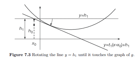
Proof. It is clear that the essential domain of $g$ is convex. We give the proof of the theorem in one dimension, so that $D(g)=I$ is an interval. Without loss of generality we may assume that $I$ is an open interval. We shall prove that for all $x_{0} \in I, g\left(x_{0}\right) \leqslant \liminf {x \rightarrow x{0}} g(x)$ and $g\left(x_{0}\right) \geqslant \limsup {x \rightarrow x{0}} g(x)$.
To prove that $g\left(x_{0}\right) \leqslant \liminf {x \rightarrow x{0}} g(x)$, suppose to the contrary that $g\left(x_{0}\right)>\liminf {x \rightarrow x{0}} g(x)$. If there were to exist $x_{1}<x_{0}<x_{2}$ such that $g\left(x_{1}\right)<g\left(x_{0}\right)$ and $g\left(x_{2}\right)<g\left(x_{0}\right)$ then
$$
g\left(x_{0}\right) \leqslant \frac{x_{2}-x_{0}}{x_{2}-x_{1}} g\left(x_{1}\right)+\frac{x_{0}-x_{1}}{x_{2}-x_{1}} g\left(x_{2}\right)<g\left(x_{0}\right)
$$
which is a contradiction. We conclude that $g(x) \geqslant g\left(x_{0}\right)$, either for all $x \geqslant x_{0}$ or for all $x \leqslant x_{0}$. Both cases are similar. We consider only the first. We may assumẻ that therrê êxists a sęuuencê $\left{\bar{x}{n}\right}$ such that $x{n} \sim_{n} x_{0}$ and $g\left(x_{n}\right) \rightarrow$
$\liminf {x \rightarrow x{0}}[g(x)]x_{0}$ we have (see figure $7.1)$
$$
g\left(x_{0}\right) \leqslant \frac{\tilde{x}-x_{0}}{\tilde{x} \quad x_{n}} g\left(x_{n}\right)+\frac{x_{0}-x_{n}}{\tilde{x} \quad x_{n}} g(\tilde{x}) .
$$
As $x_{n} \rightarrow x_{0}$ the right hand side tends to $\liminf {x \rightarrow x{0}} g(x)$ which contradicts the assumption.
物理代写|统计力学代写Statistical mechanics代考|Thermodynamic Potentials
After the preliminaries about convex functions in chapter 7 , we can now define the free energy density $f(v, T)$ as minus the Legendre transform of $u(s, v)$ with respect to the variable $s$ :
$$
f(v, T)=-\sup {s}{T s-u(s, v)} . $$ It is easy to see that the function $u(s, v)$ is convex so that we can use theorem $7.2$ to invert the Legendre transform and write $$ u(s, v)=\sup {T}{T s+f(v, T)} .
$$
Note that we can also write
$$
f(v, T)=\inf {u}{u-T s(u, v)} $$ that is, $-(1 / T) f(v, T)$ is the Legendre transform of $-s(u, v)$. Inverting this relation we obtain $$ s(u, v)=\inf {T>0} \frac{1}{T}{u-f(v, T)} .
$$
The free energy density is an important quantity in thermodynamics because in many experimental situations it is easier to control the temperature than the internal energy. Note that the supremum in (8.1) is attained at the value of $s$ satisfying (6.8) so that it is legitimate to denote the variable $T$ in the free energy density as the temperature. We can therefore write
$$
f(v, T)=u(s(v, T), v)-T s(v, T),
$$
where $s(v, T)$ is defined as the solution of (6.8). Alternatively,
$$
f(v, T)=u(v, T)-T s(u(v, T), v)
$$
where $u(v, T)$ is the solution of
$$
\frac{1}{T}=\left(\frac{\partial s}{\partial u}\right){v} $$ Differentiating (8.5) w.r.t. to $v$ we obtain, using equations (6.8) and $(6.9)$, $$ \left(\frac{\partial f}{\partial v}\right){T}(v, T)=\left(\frac{\partial u}{\partial v}\right){s}(s(v, T), v)=-p(v, T) $$ Similarly we have $$ \left(\frac{\partial f}{\partial T}\right){v}=-s(v, T)
$$
so that we can write
$$
\mathrm{d} f=-p \mathrm{~d} v-s \mathrm{~d} T
$$
Note that this implies in particular that for an isothermal process from an equilibrium state $\alpha$ to an equilibrium state $\beta$, the work done per particle $w$ equals
$$
w=f(\beta)-f(\alpha)
$$
Thus, the free energy plays a role similar to the potential energy in mechanics: given the work done in an isothermal process, (8.11) determines the new equilibrium state.
In some cases it is convenient to work in terms of the variables $s$ and $p$. We then take a Legendre transform with respect to $v$ and define the enthalpy $h(s, p)$ by
$$
h(s, p)=\inf _{v}{p v+u(s, v)}
$$
It is easy to prove that
$$
\mathrm{d} h=\delta q+v \mathrm{~d} p
$$
物理代写|统计力学代写Statistical mechanics代考|Phase Transitions
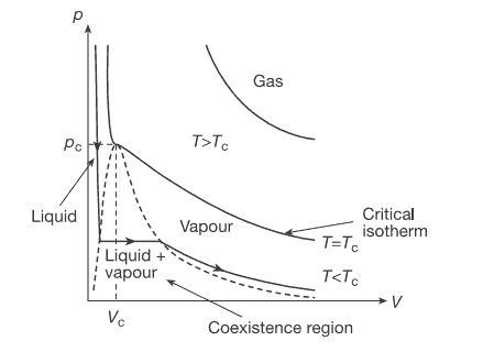
Consider again the $p-V$ diagram for a general fluid given as figure 1 in the introduction. In the region under the broken curve, liquid and vapour (gas at temperatures below $T_{c}$ is usually called vapour) coexist. As the volume is increased in this region the pressure remains constant and liquid vaporizes (figure 9.1).
It follows that the pressure at which liquid and vapour coexist is a function of the temperature alone. If the temperature of the liquid is raised while keeping the pressure above the liquid constant, it will no longer be in equilibrium and will evaporate. If we want to keep it in equilibrium, we must increase the pressure. The equilibrium pressure is therefore an increasing function of the temperature. The graph of this function is the line of coexistence of liquid and vapour shown in figure $9.2$. Above this line, only liquid exists in equilibrium while below the curve only vapour exists in equilibrium. This argument also shows that by lowering the pressure above a liquid its boiling point decreases. This is an important method for obtaining low temperatures (refrigeration). For example, by pumping away the vapour above liquid helium-3 $\left({ }^{3} \mathrm{He}\right.$ ) (a rare isotope of helium), one can reduce the temperature by an order of magnitude, from approximately $3 \mathrm{~K}$ to $0.3 \mathrm{~K}$.
Another look at the $p-V$ diagram shows that the coexistence curve must end at a maximum temperature $T_{c}$ called the critical temperature. This point of the coexistence curve $p_{e q}(T)$ corresponds to one single point $\left(p_{c}, V_{c}\right)$ in the $p-V$ diagram, the critical point. At this point remarkable things happen: the so called critical phenomena. For example, the isothermal compressibility $\kappa_{T}$ (see equation (4.14)) diverges at the critical point. Also the specific heat $c_{V}$ diverges. This means that the free energy is not twice differentiable at the critical point. One therefore speaks of a second-order phase transition. The degree of divergence can be expressed in terms of critical exponents. It turns out that $\kappa_{T}$ and $c_{V}$ behave near the critical point asymptotically as
$$
\kappa_{T} \sim \mathcal{K}\left|’ I^{\prime}-H_{c}^{\prime}\right|^{-\gamma}
$$
统计力学代考
物理代写|统计力学代写Statistical mechanics代考|Convexity
内能函数的凸性是直接关系到热力学平衡稳定性的重要性质。在本章中,我们推导出凸函数的一些性质,这将使我们能够进一步发展热力学理论。我们一般地陈述这些定理,但只给出一维情况的证明。一般证明ķ维情况可以在附录C中找到。无论如何,尽管定义、概念和定理是理解后续理论的必要证明,但证明并不是必不可少的。
我们从一个定义开始。
如果G:Rķ→R∪+∞是一个可以取值的函数+∞然后定义它的基本域
D(g)=\left{\vec{x} \in \mathbb{R}^{k} \mid g(\vec{x})<+\infty\right} 。D(g)=\left{\vec{x} \in \mathbb{R}^{k} \mid g(\vec{x})<+\infty\right} 。
定理 7.1 一个凸函数G:Rķ→R∪+∞在其本质域的每个内部点上是连续的。
证明。很明显,基本领域G是凸的。我们在一维上给出定理的证明,所以D(G)=我是一个区间。不失一般性,我们可以假设我是一个开区间。我们将证明对所有人X0∈我,G(X0)⩽林信息X→X0G(X)和G(X0)⩾林汤X→X0G(X).
为了证明G(X0)⩽林信息X→X0G(X), 假设相反G(X0)>林信息X→X0G(X). 如果存在X1<X0<X2这样G(X1)<G(X0)和G(X2)<G(X0)然后
G(X0)⩽X2−X0X2−X1G(X1)+X0−X1X2−X1G(X2)<G(X0)
这是一个矛盾。我们得出结论G(X)⩾G(X0), 要么对所有人X⩾X0或为所有人X⩽X0. 两种情况都是相似的。我们只考虑第一个。我们可以假设 therrê ê 存在一个 sęuuencê\left{\bar{x}{n}\right}\left{\bar{x}{n}\right}这样Xn∼nX0和G(Xn)→
林信息X→X0[G(X)]X0我们有(见图7.1)
G(X0)⩽X~−X0X~XnG(Xn)+X0−XnX~XnG(X~).
作为Xn→X0右手边倾向于林信息X→X0G(X)这与假设相矛盾。
物理代写|统计力学代写Statistical mechanics代考|Thermodynamic Potentials
在第 7 章中关于凸函数的初步介绍之后,我们现在可以定义自由能密度了。F(在,吨)减去勒让德变换在(s,在)关于变量s :
F(在,吨)=−支持s吨s−在(s,在).很容易看出函数在(s,在)是凸的,所以我们可以使用定理7.2反转勒让德变换并写入
在(s,在)=支持吨吨s+F(在,吨).
注意我们也可以写
F(在,吨)=信息在在−吨s(在,在)那是,−(1/吨)F(在,吨)是勒让德变换−s(在,在). 反转这个关系,我们得到
s(在,在)=信息吨>01吨在−F(在,吨).
自由能密度是热力学中的一个重要量,因为在许多实验情况下,控制温度比控制内能更容易。请注意,(8.1)中的上确界是在以下值处获得的s满足(6.8),因此表示变量是合法的吨在自由能密度中作为温度。因此我们可以写
F(在,吨)=在(s(在,吨),在)−吨s(在,吨),
在哪里s(在,吨)定义为 (6.8) 的解。或者,
F(在,吨)=在(在,吨)−吨s(在(在,吨),在)
在哪里在(在,吨)是解决方案
1吨=(∂s∂在)在将 (8.5) 微分到在我们得到,使用方程(6.8)和(6.9),
(∂F∂在)吨(在,吨)=(∂在∂在)s(s(在,吨),在)=−p(在,吨)同样我们有
(∂F∂吨)在=−s(在,吨)
这样我们就可以写
dF=−p d在−s d吨
请注意,这尤其意味着对于从平衡状态开始的等温过程一个达到平衡状态b, 每个粒子所做的功在等于
在=F(b)−F(一个)
因此,自由能在力学中起着类似于势能的作用:给定在等温过程中所做的功,(8.11) 决定了新的平衡状态。
在某些情况下,根据变量工作很方便s和p. 然后我们对以下内容进行勒让德变换在并定义焓H(s,p)经过
H(s,p)=信息在p在+在(s,在)
很容易证明
dH=dq+在 dp
物理代写|统计力学代写Statistical mechanics代考|Phase Transitions
再次考虑p−在介绍中图 1 给出的一般流体图。在折断曲线下的区域,液体和蒸汽(温度低于吨C通常称为蒸汽)共存。随着该区域的体积增加,压力保持恒定,液体蒸发(图 9.1)。
由此可见,液体和蒸汽共存的压力是单独温度的函数。如果在保持液体上方压力恒定的情况下提高液体温度,它将不再处于平衡状态并会蒸发。如果我们想保持平衡,我们必须增加压力。因此,平衡压力是温度的增函数。该函数的图形是如图所示的液体和蒸汽共存线9.2. 在这条线之上,只有液体处于平衡状态,而在曲线之下,只有蒸汽处于平衡状态。这一论点还表明,通过降低液体以上的压力,其沸点会降低。这是获得低温(冷藏)的重要方法。例如,通过抽走液态氦 3 上方的蒸汽(3H和)(氦的一种稀有同位素),可以将温度降低一个数量级,从大约3 ķ至0.3 ķ.
再看看p−在图显示共存曲线必须在最高温度结束吨C称为临界温度。共存曲线的这一点p和q(吨)对应一个点(pC,在C)在里面p−在图,关键点。在这一点上发生了非凡的事情:所谓的临界现象。例如,等温可压缩性ķ吨(见方程(4.14))在临界点发散。还有比热C在分歧。这意味着自由能在临界点不是两次可微的。因此有人谈到二阶相变。分歧程度可以用临界指数来表示。事实证明ķ吨和C在在临界点附近表现得渐近为
ķ吨∼ķ|′我′−HC′|−C

统计代写请认准statistics-lab™. statistics-lab™为您的留学生涯保驾护航。
金融工程代写
金融工程是使用数学技术来解决金融问题。金融工程使用计算机科学、统计学、经济学和应用数学领域的工具和知识来解决当前的金融问题,以及设计新的和创新的金融产品。
非参数统计代写
非参数统计指的是一种统计方法,其中不假设数据来自于由少数参数决定的规定模型;这种模型的例子包括正态分布模型和线性回归模型。
广义线性模型代考
广义线性模型(GLM)归属统计学领域,是一种应用灵活的线性回归模型。该模型允许因变量的偏差分布有除了正态分布之外的其它分布。
术语 广义线性模型(GLM)通常是指给定连续和/或分类预测因素的连续响应变量的常规线性回归模型。它包括多元线性回归,以及方差分析和方差分析(仅含固定效应)。
有限元方法代写
有限元方法(FEM)是一种流行的方法,用于数值解决工程和数学建模中出现的微分方程。典型的问题领域包括结构分析、传热、流体流动、质量运输和电磁势等传统领域。
有限元是一种通用的数值方法,用于解决两个或三个空间变量的偏微分方程(即一些边界值问题)。为了解决一个问题,有限元将一个大系统细分为更小、更简单的部分,称为有限元。这是通过在空间维度上的特定空间离散化来实现的,它是通过构建对象的网格来实现的:用于求解的数值域,它有有限数量的点。边界值问题的有限元方法表述最终导致一个代数方程组。该方法在域上对未知函数进行逼近。[1] 然后将模拟这些有限元的简单方程组合成一个更大的方程系统,以模拟整个问题。然后,有限元通过变化微积分使相关的误差函数最小化来逼近一个解决方案。
tatistics-lab作为专业的留学生服务机构,多年来已为美国、英国、加拿大、澳洲等留学热门地的学生提供专业的学术服务,包括但不限于Essay代写,Assignment代写,Dissertation代写,Report代写,小组作业代写,Proposal代写,Paper代写,Presentation代写,计算机作业代写,论文修改和润色,网课代做,exam代考等等。写作范围涵盖高中,本科,研究生等海外留学全阶段,辐射金融,经济学,会计学,审计学,管理学等全球99%专业科目。写作团队既有专业英语母语作者,也有海外名校硕博留学生,每位写作老师都拥有过硬的语言能力,专业的学科背景和学术写作经验。我们承诺100%原创,100%专业,100%准时,100%满意。
随机分析代写
随机微积分是数学的一个分支,对随机过程进行操作。它允许为随机过程的积分定义一个关于随机过程的一致的积分理论。这个领域是由日本数学家伊藤清在第二次世界大战期间创建并开始的。
时间序列分析代写
随机过程,是依赖于参数的一组随机变量的全体,参数通常是时间。 随机变量是随机现象的数量表现,其时间序列是一组按照时间发生先后顺序进行排列的数据点序列。通常一组时间序列的时间间隔为一恒定值(如1秒,5分钟,12小时,7天,1年),因此时间序列可以作为离散时间数据进行分析处理。研究时间序列数据的意义在于现实中,往往需要研究某个事物其随时间发展变化的规律。这就需要通过研究该事物过去发展的历史记录,以得到其自身发展的规律。
回归分析代写
多元回归分析渐进(Multiple Regression Analysis Asymptotics)属于计量经济学领域,主要是一种数学上的统计分析方法,可以分析复杂情况下各影响因素的数学关系,在自然科学、社会和经济学等多个领域内应用广泛。
MATLAB代写
MATLAB 是一种用于技术计算的高性能语言。它将计算、可视化和编程集成在一个易于使用的环境中,其中问题和解决方案以熟悉的数学符号表示。典型用途包括:数学和计算算法开发建模、仿真和原型制作数据分析、探索和可视化科学和工程图形应用程序开发,包括图形用户界面构建MATLAB 是一个交互式系统,其基本数据元素是一个不需要维度的数组。这使您可以解决许多技术计算问题,尤其是那些具有矩阵和向量公式的问题,而只需用 C 或 Fortran 等标量非交互式语言编写程序所需的时间的一小部分。MATLAB 名称代表矩阵实验室。MATLAB 最初的编写目的是提供对由 LINPACK 和 EISPACK 项目开发的矩阵软件的轻松访问,这两个项目共同代表了矩阵计算软件的最新技术。MATLAB 经过多年的发展,得到了许多用户的投入。在大学环境中,它是数学、工程和科学入门和高级课程的标准教学工具。在工业领域,MATLAB 是高效研究、开发和分析的首选工具。MATLAB 具有一系列称为工具箱的特定于应用程序的解决方案。对于大多数 MATLAB 用户来说非常重要,工具箱允许您学习和应用专业技术。工具箱是 MATLAB 函数(M 文件)的综合集合,可扩展 MATLAB 环境以解决特定类别的问题。可用工具箱的领域包括信号处理、控制系统、神经网络、模糊逻辑、小波、仿真等。