如果你也在 怎样代写计量经济学Econometrics这个学科遇到相关的难题,请随时右上角联系我们的24/7代写客服。
计量经济学是将统计方法应用于经济数据,以赋予经济关系以经验内容。
statistics-lab™ 为您的留学生涯保驾护航 在代写计量经济学Econometrics方面已经树立了自己的口碑, 保证靠谱, 高质且原创的统计Statistics代写服务。我们的专家在代写计量经济学Econometrics代写方面经验极为丰富,各种代写计量经济学Econometrics相关的作业也就用不着说。
我们提供的计量经济学Econometrics及其相关学科的代写,服务范围广, 其中包括但不限于:
- Statistical Inference 统计推断
- Statistical Computing 统计计算
- Advanced Probability Theory 高等楖率论
- Advanced Mathematical Statistics 高等数理统计学
- (Generalized) Linear Models 广义线性模型
- Statistical Machine Learning 统计机器学习
- Longitudinal Data Analysis 纵向数据分析
- Foundations of Data Science 数据科学基础
- Statistical Inference 统计推断
- Statistical Computing 统计计算
- Advanced Probability Theory 高等楖率论
- Advanced Mathematical Statistics 高等数理统计学
- (Generalized) Linear Models 广义线性模型
- Statistical Machine Learning 统计机器学习
- Longitudinal Data Analysis 纵向数据分析
- Foundations of Data Science 数据科学基础
经济代写|计量经济学作业代写Econometrics代考|Consistency and Laws of Large Numbers
We begin this scetion by introducing the notion of consistency, one of the most basic ideas of asymptotic theory. When one is interested in estimating parameters from data, it is desirable that the parameter estimates should have certain properties. In Chapters 2 and 3 , we saw that, under certain regularity
conditions, the OLS estimator is unbiased and follows a normal distribution with a covariance matrix that is known up to a factor of the error variance, which factor can itself be estimated in an unbiased manner. We were not able in those chapters to prove any corresponding results for the NLS estimator, and it was remarked that asymptotic theory would be necessary in order to do so. Consistency is the first of the desirable asymptotic properties that an estimator may possess. In Chapter 5 we will provide conditions under which the NLS estimator is consistent. Here we will content ourselves with introducing the notion itself and illustrating the close link that exists between laws of large numbers and proofs of consistency.
An estimator $\hat{\beta}$ of a vector of parameters $\beta$ is said to be consistent if it converges to its true value as the sample size tends to infinity. That statement is not false or even seriously misleading, but it implicitly makes a number of assumptions and uses undefined terms. Let us try to rectify this and, in so doing, gain a better understanding of what consistency means.
First, how can an estimator converge? It can do so if we convert it to a sequence. To this end, we write $\hat{\beta}^{n}$ for the estimator that results from a sample of size $n$ and then define the estimator $\hat{\beta}$ itself as the sequence $\left{\hat{\beta}^{n}\right}_{n=m \text {. }}$. The lower limit $m$ of the sequence will usually be assumed to be the smallest sample size that allows $\hat{\beta}^{n}$ to be computed. For example, if we denote the regressand and regressor matrix for a linear regression done on a sample of size $n$ by $\boldsymbol{y}^{n}$ and $\boldsymbol{X}^{n}$, respectively, and if $\boldsymbol{X}^{n}$ is an $n \times k$ matrix, then $m$ cannot be any smaller than $k$, the number of regressors. For $n>k$ we have as usual that $\hat{\beta}^{n}=\left(\left(\boldsymbol{X}^{n}\right)^{\top} \boldsymbol{X}^{n}\right)^{-1}\left(\boldsymbol{X}^{n}\right)^{\top} \boldsymbol{y}^{n}$, and this formula embodies the rule which generates the sequence $\hat{\beta}$.
An element of a sequence $\hat{\boldsymbol{\beta}}$ is a random variable. If it is to converge to a true value, we must say what kind of convergence we have in mind. since we have seen that more than one kind is available. If we use almost sure convergence, we will say that we have strong consistency or that the estimator is strongly consistent. Sometimes such a claim is possible. More frequently we use convergence in probability and so obtain only weak consistency. Here “strong” and “weak” are used in the same sense as in the definitions of strong and weak laws of large numbers.
Next, what is meant by the “true value”? We answer this question in detail in the next chapter, but here we must at least note that convergence of a sequence of random variables to any kind of limit depends on the rule, or DGP, which generated the sequence. For example, if the rule ensures that, for any sample size $n$, the regressand and regressor matrix of a linear regression are in fact related by the equation
$$
\boldsymbol{y}^{n}=\boldsymbol{X}^{n} \beta_{0}+\boldsymbol{u}^{n}
$$
for some fixed vector $\beta_{0}$, with $\boldsymbol{u}^{n}$ an $n$-vector of white noise errors, then the true value for this DGP will be $\beta_{0}$. The estimator $\hat{\beta}$, to be consistent, should
converge, under the $\operatorname{DGP}(4.19)$, to $\beta_{0}$ whatever the fixed value $\beta_{0}$ happens to be. However, if the DGP is such that (4.19) does not hold for any $\boldsymbol{\beta}_{0}$ at all, then we cannot give any meaning to the term “consistency” as we are using it at present.
After this preamble, we can finally investigate consistency in a particular case. We could take as an example the linear regression (4.19), but that would lead us into consideration of too many side issues that will be dealt with in the next chapter. Instead, we will consider the very instructive example that is afforded by the Fundamental Theorem of Statistics, a simple version of which we will now prove. This theorem, which is indeed fundamental to all statistical inference, states that if we sample randomly with replacement from a population, the empirical distribution function is consistent for the population distribution function.
Let us formalize this statement and then prove it. The term population is used in its statistical sense of a set, finite or infinite, from which independent random draws can be made. Each such draw is a member of the population. By random sampling with replacement is meant a procedure which ensures that in each draw the probability that any given member of the population is drawn is unchanging. A random sample will be a finite set of draws. Formally, the population is represented by a c.d.f. $F(x)$ for a scalar random variable $x$. The draws from the population are identified with different, independent, realizations of $x$.
经济代写|计量经济学作业代写Econometrics代考|6 Asymptotic Normality and Central Limit Theorems
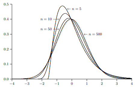
There is the same sort of close connection between the property of asymptotic normality and central limit theorems as there is between consistency and laws of large numbers. The easiest way to demonstrate this close connection is by means of an example. Suppose that samples are generated by random drawings from distributions with an unknown mean $\mu$ and unknown and variable variances. For example, it might be that the variance of the distribution from which the $t^{\text {th }}$ observation is drawn is
$$
\sigma_{t}^{2} \equiv \omega^{2}\left(1+\frac{1}{2}(t(\bmod 3))\right) .
$$
Then $\sigma_{t}^{2}$ will take on the values $\omega^{2}, 1.5 \omega^{2}$, and $2 \omega^{2}$ with equal probability. Thus $\sigma_{t}^{2}$ varies systematically with $t$ but always remains within certain limits, in this case $\omega^{2}$ and $2 \omega^{2}$.
We will suppose that the investigator does not know the exact relation (4.26) and is prepared to assume only that the variances $\sigma_{t}^{2}$ vary between two positive bounds and average out asymptotically to some value $\sigma_{0}^{2}$, which may or not be known, defined as
$$
\sigma_{0}^{2} \equiv \lim {n \rightarrow \infty}\left(\frac{1}{n} \sum{t=1}^{n} \sigma_{t}^{2}\right)
$$
The sample mean may still be used as an estimator of the population mean, since our law of large numbers, Theorem 4.1, is applicable. The investigator is also prepared to assume that the distributions from which the observations are drawn have absolute third moments that are bounded, and so we too will assume that this is so. The investigator wishes to perform asymptotic statistical inference on the estimate derived from a realized sample and is therefore
interested in the nondegenerate asymptotic distribution of the sample mean as an estimator. We saw in Section $4.3$ that for this purpose we should look at the distribution of $n^{1 / 2}\left(m_{1}-\mu\right)$, where $m_{1}$ is the sample mean. Specifically, we wish to study
$$
n^{1 / 2}\left(m_{1}-\mu\right)=n^{-1 / 2} \sum_{t=1}^{n}\left(y_{t}-\mu\right),
$$
where $y_{t}-\mu$ has variance $\sigma_{t}^{2}$.
We begin by stating the following simple central limit theorem.
Theorem 4.2. Simple Central Limit Theorem. (Lyapunov)
Let $\left{y_{t}\right}$ be a sequence of independent, centered random variables with variances $\sigma_{t}^{2}$ such that $\sigma^{2} \leq \sigma_{t}^{2} \leq \bar{\sigma}^{2}$ for two finite positive constants, $\sigma^{2}$ and $\bar{\sigma}^{2}$, and absolute third moments $\mu_{3}$ such that $\mu_{3} \leq \bar{\mu}{3}$ for a finite constant $\bar{\mu}{3}$. Further, let
$$
\sigma_{0}^{2} \equiv \lim {n \rightarrow \infty}\left(\frac{1}{n} \sum{t=1}^{n} \sigma_{t}^{2}\right)
$$
exist. Then the sequence
$$
\left{n^{-1 / 2} \sum_{t=1}^{n} y_{t}\right}
$$
tends in distribution to a limit characterized by the normal distribution with mean zero and variance $\sigma_{0}^{2}$.
经济代写|计量经济学作业代写Econometrics代考|Some Useful Results
This section is intended to serve as a reference for much of the rest of the book. We will essentially make a list (with occasional commentary but without proofs) of useful definitions and theorems. At the end of this we will present two sets of regularity conditions that will each have a set of desirable implications. Later, we will be able to make assumptions by which one or other of these whole sets of regularity conditions is satisfied and thereby be able to draw without further ado a wide variety of useful conclusions.
To begin with, we will concentrate on laws of large numbers and the properties that allow them to be satisfied. In all of these theorems, we consider a sequence of sums $\left{S_{n}\right}$ where
$$
S_{n}=\frac{1}{n} \sum_{t=1}^{n} y_{t}
$$
The random variables $y_{t}$ will be referred to as the (random) summands. First, we present a theorem with very little in the way of moment restrictions on the random summands but very strong restrictions on their homogeneity.
Theorem 4.3. (Khinchin)
If the random variables $y_{t}$ of the sequence $\left{y_{t}\right}$ are mutually independent and all distributed according to the same distribution, which possesses a mean of $\mu$, then
$$
\operatorname{Pr}\left(\lim {n \rightarrow \infty} S{n}=\mu\right)=1
$$
Only the existence of the first moment is required, but all the summands must be identically distributed. Notice that the identical mean of the summands means that we need not bother to center the variables $y_{t}$.
Next, we present a theorem due to Kolmogorov, which still requires independence of the summands, and now existence of their second moments, but very little else in the way of homogeneity.
计量经济学代考
经济代写|计量经济学作业代写Econometrics代考|Consistency and Laws of Large Numbers
我们首先介绍一致性的概念,这是渐近理论的最基本概念之一。当人们对从数据中估计参数感兴趣时,希望参数估计应该具有某些属性。在第 2 章和第 3 章中,我们看到,在一定的规律下
条件下,OLS 估计量是无偏的,并且遵循具有已知误差方差因子的协方差矩阵的正态分布,该因子本身可以以无偏的方式估计。在那些章节中,我们无法证明 NLS 估计量的任何相应结果,并且有人指出,为了做到这一点,渐近理论是必要的。一致性是估计器可能拥有的第一个理想的渐近属性。在第 5 章中,我们将提供 NLS 估计量一致的条件。在这里,我们将满足于介绍这个概念本身并说明大数定律和一致性证明之间存在的密切联系。
估算器b^参数向量的b当样本量趋于无穷大时,如果它收敛到其真实值,则称它是一致的。该陈述不是错误的,甚至不是严重的误导,但它隐含地做出了一些假设并使用了未定义的术语。让我们尝试纠正这一点,并在此过程中更好地理解一致性的含义。
首先,估计器如何收敛?如果我们将其转换为序列,它就可以做到这一点。为此,我们写b^n对于从大小样本产生的估计量n然后定义估计器b^本身作为序列\left{\hat{\beta}^{n}\right}_{n=m \text {. }}\left{\hat{\beta}^{n}\right}_{n=m \text {. }}. 下限米通常将假定序列的最小样本量允许b^n要计算。例如,如果我们表示对大小样本进行线性回归的回归和回归矩阵n经过是n和Xn,分别,如果Xn是一个n×ķ矩阵,那么米不能小于ķ,回归变量的数量。为了n>ķ我们像往常一样b^n=((Xn)⊤Xn)−1(Xn)⊤是n, 这个公式体现了生成序列的规则b^.
序列的一个元素b^是一个随机变量。如果要收敛到一个真实的值,我们必须说我们想到了什么样的收敛。因为我们已经看到不止一种可用。如果我们使用几乎肯定的收敛,我们会说我们具有强一致性或估计量是强一致的。有时这样的主张是可能的。我们更频繁地使用概率收敛,因此只能获得弱一致性。这里“强”和“弱”的使用意义与大数强定律和弱定律的定义相同。
其次,什么是“真值”?我们将在下一章详细回答这个问题,但在这里我们至少必须注意,随机变量序列收敛到任何类型的极限取决于生成序列的规则或 DGP。例如,如果规则确保对于任何样本量n,线性回归的regressand和regressor矩阵实际上是由方程相关的
是n=Xnb0+在n
对于一些固定向量b0, 和在n一个n-白噪声误差向量,则此 DGP 的真实值将是b0. 估算器b^,为了保持一致,应该
收敛,下DGP(4.19), 到b0无论是固定值b0恰好是。然而,如果 DGP 使得 (4.19) 不成立b0根本上,我们无法赋予我们目前使用的“一致性”一词任何含义。
在这个序言之后,我们终于可以研究特定情况下的一致性。我们可以将线性回归(4.19)作为一个例子,但这会导致我们考虑太多的附带问题,这些问题将在下一章中讨论。相反,我们将考虑统计基本定理提供的非常有启发性的例子,我们现在将证明它的一个简单版本。这个定理确实是所有统计推断的基础,它指出如果我们从总体中随机抽样并放回,经验分布函数与总体分布函数是一致的。
让我们形式化这个陈述然后证明它。人口一词是在其统计意义上使用的一组有限或无限的,可以从中进行独立的随机抽取。每个这样的抽签都是人口中的一员。带放回的随机抽样是指确保在每次抽签中抽取任何给定总体成员的概率不变的程序。随机样本将是一组有限的抽奖。形式上,人口由 cdf 表示F(X)对于标量随机变量X. 来自人口的抽签被识别为不同的、独立的、实现的X.
经济代写|计量经济学作业代写Econometrics代考|6 Asymptotic Normality and Central Limit Theorems
渐近正态性的性质和中心极限定理之间有着同样的密切联系,正如一致性和大数定律之间的联系一样。演示这种紧密联系的最简单方法是通过示例。假设样本是从具有未知均值的分布中随机抽取的μ以及未知和可变的方差。例如,可能是分布的方差吨th 观察结果是
σ吨2≡ω2(1+12(吨(反对3))).
然后σ吨2将采用价值观ω2,1.5ω2, 和2ω2以相等的概率。因此σ吨2系统地变化吨但始终保持在一定的范围内,在这种情况下ω2和2ω2.
我们将假设调查员不知道确切的关系(4.26),并准备仅假设方差σ吨2在两个正边界之间变化并逐渐平均到某个值σ02,可能已知或未知,定义为
σ02≡林n→∞(1n∑吨=1nσ吨2)
样本均值仍可用作总体均值的估计量,因为我们的大数定律(定理 4.1)适用。调查人员还准备假设从中得出观察结果的分布具有绝对的三次矩,这是有界的,因此我们也将假设情况如此。调查人员希望对从已实现样本得出的估计值进行渐近统计推断,因此
对作为估计量的样本均值的非退化渐近分布感兴趣。我们在章节中看到4.3为了这个目的,我们应该看看分布n1/2(米1−μ), 在哪里米1是样本均值。具体来说,我们希望研究
n1/2(米1−μ)=n−1/2∑吨=1n(是吨−μ),
在哪里是吨−μ有方差σ吨2.
我们首先陈述以下简单的中心极限定理。
定理 4.2。简单中心极限定理。(李雅普诺夫)
让\left{y_{t}\right}\left{y_{t}\right}是一系列具有方差的独立中心随机变量σ吨2这样σ2≤σ吨2≤σ¯2对于两个有限的正常数,σ2和σ¯2, 和绝对的第三时刻μ3这样μ3≤μ¯3对于有限常数μ¯3. 此外,让
σ02≡林n→∞(1n∑吨=1nσ吨2)
存在。然后是序列
\left{n^{-1 / 2} \sum_{t=1}^{n} y_{t}\right}\left{n^{-1 / 2} \sum_{t=1}^{n} y_{t}\right}
分布趋于以均值为零和方差的正态分布为特征的极限σ02.
经济代写|计量经济学作业代写Econometrics代考|Some Useful Results
本节旨在作为本书其余部分的参考。我们基本上将列出有用的定义和定理(偶尔有评论但没有证明)。最后,我们将提出两组规律性条件,每一个都具有一组理想的含义。稍后,我们将能够做出满足这些整套规律性条件中的一个或另一个的假设,从而能够毫不费力地得出各种有用的结论。
首先,我们将专注于大数定律和使它们得到满足的性质。在所有这些定理中,我们考虑一系列和\left{S_{n}\right}\left{S_{n}\right}在哪里
小号n=1n∑吨=1n是吨
随机变量是吨将被称为(随机)加法。首先,我们提出了一个定理,对随机和的矩限制很少,但对它们的同质性有很强的限制。
定理 4.3。(Khinchin)
如果随机变量是吨序列的\left{y_{t}\right}\left{y_{t}\right}是相互独立的,并且都按照相同的分布进行分布,其均值为μ, 然后
公关(林n→∞小号n=μ)=1
只需要第一时刻的存在,但所有的和必须同分布。请注意,和的相同平均值意味着我们无需费心将变量居中是吨.
接下来,我们提出一个由于 Kolmogorov 的定理,它仍然需要被加数的独立性,现在它们的二阶矩存在,但在同质性方面几乎没有其他东西。

统计代写请认准statistics-lab™. statistics-lab™为您的留学生涯保驾护航。
随机过程代考
在概率论概念中,随机过程是随机变量的集合。 若一随机系统的样本点是随机函数,则称此函数为样本函数,这一随机系统全部样本函数的集合是一个随机过程。 实际应用中,样本函数的一般定义在时间域或者空间域。 随机过程的实例如股票和汇率的波动、语音信号、视频信号、体温的变化,随机运动如布朗运动、随机徘徊等等。
贝叶斯方法代考
贝叶斯统计概念及数据分析表示使用概率陈述回答有关未知参数的研究问题以及统计范式。后验分布包括关于参数的先验分布,和基于观测数据提供关于参数的信息似然模型。根据选择的先验分布和似然模型,后验分布可以解析或近似,例如,马尔科夫链蒙特卡罗 (MCMC) 方法之一。贝叶斯统计概念及数据分析使用后验分布来形成模型参数的各种摘要,包括点估计,如后验平均值、中位数、百分位数和称为可信区间的区间估计。此外,所有关于模型参数的统计检验都可以表示为基于估计后验分布的概率报表。
广义线性模型代考
广义线性模型(GLM)归属统计学领域,是一种应用灵活的线性回归模型。该模型允许因变量的偏差分布有除了正态分布之外的其它分布。
statistics-lab作为专业的留学生服务机构,多年来已为美国、英国、加拿大、澳洲等留学热门地的学生提供专业的学术服务,包括但不限于Essay代写,Assignment代写,Dissertation代写,Report代写,小组作业代写,Proposal代写,Paper代写,Presentation代写,计算机作业代写,论文修改和润色,网课代做,exam代考等等。写作范围涵盖高中,本科,研究生等海外留学全阶段,辐射金融,经济学,会计学,审计学,管理学等全球99%专业科目。写作团队既有专业英语母语作者,也有海外名校硕博留学生,每位写作老师都拥有过硬的语言能力,专业的学科背景和学术写作经验。我们承诺100%原创,100%专业,100%准时,100%满意。
机器学习代写
随着AI的大潮到来,Machine Learning逐渐成为一个新的学习热点。同时与传统CS相比,Machine Learning在其他领域也有着广泛的应用,因此这门学科成为不仅折磨CS专业同学的“小恶魔”,也是折磨生物、化学、统计等其他学科留学生的“大魔王”。学习Machine learning的一大绊脚石在于使用语言众多,跨学科范围广,所以学习起来尤其困难。但是不管你在学习Machine Learning时遇到任何难题,StudyGate专业导师团队都能为你轻松解决。
多元统计分析代考
基础数据: $N$ 个样本, $P$ 个变量数的单样本,组成的横列的数据表
变量定性: 分类和顺序;变量定量:数值
数学公式的角度分为: 因变量与自变量
时间序列分析代写
随机过程,是依赖于参数的一组随机变量的全体,参数通常是时间。 随机变量是随机现象的数量表现,其时间序列是一组按照时间发生先后顺序进行排列的数据点序列。通常一组时间序列的时间间隔为一恒定值(如1秒,5分钟,12小时,7天,1年),因此时间序列可以作为离散时间数据进行分析处理。研究时间序列数据的意义在于现实中,往往需要研究某个事物其随时间发展变化的规律。这就需要通过研究该事物过去发展的历史记录,以得到其自身发展的规律。
回归分析代写
多元回归分析渐进(Multiple Regression Analysis Asymptotics)属于计量经济学领域,主要是一种数学上的统计分析方法,可以分析复杂情况下各影响因素的数学关系,在自然科学、社会和经济学等多个领域内应用广泛。
MATLAB代写
MATLAB 是一种用于技术计算的高性能语言。它将计算、可视化和编程集成在一个易于使用的环境中,其中问题和解决方案以熟悉的数学符号表示。典型用途包括:数学和计算算法开发建模、仿真和原型制作数据分析、探索和可视化科学和工程图形应用程序开发,包括图形用户界面构建MATLAB 是一个交互式系统,其基本数据元素是一个不需要维度的数组。这使您可以解决许多技术计算问题,尤其是那些具有矩阵和向量公式的问题,而只需用 C 或 Fortran 等标量非交互式语言编写程序所需的时间的一小部分。MATLAB 名称代表矩阵实验室。MATLAB 最初的编写目的是提供对由 LINPACK 和 EISPACK 项目开发的矩阵软件的轻松访问,这两个项目共同代表了矩阵计算软件的最新技术。MATLAB 经过多年的发展,得到了许多用户的投入。在大学环境中,它是数学、工程和科学入门和高级课程的标准教学工具。在工业领域,MATLAB 是高效研究、开发和分析的首选工具。MATLAB 具有一系列称为工具箱的特定于应用程序的解决方案。对于大多数 MATLAB 用户来说非常重要,工具箱允许您学习和应用专业技术。工具箱是 MATLAB 函数(M 文件)的综合集合,可扩展 MATLAB 环境以解决特定类别的问题。可用工具箱的领域包括信号处理、控制系统、神经网络、模糊逻辑、小波、仿真等。