如果你也在 怎样代写计量经济学Econometrics这个学科遇到相关的难题，请随时右上角联系我们的24/7代写客服。

计量经济学是将统计方法应用于经济数据，以赋予经济关系以经验内容。

statistics-lab™ 为您的留学生涯保驾护航 在代写计量经济学Econometrics方面已经树立了自己的口碑, 保证靠谱, 高质且原创的统计Statistics代写服务。我们的专家在代写计量经济学Econometrics代写方面经验极为丰富，各种代写计量经济学Econometrics相关的作业也就用不着说。

我们提供的计量经济学Econometrics及其相关学科的代写，服务范围广, 其中包括但不限于:

• Statistical Inference 统计推断
• Statistical Computing 统计计算
• Advanced Probability Theory 高等楖率论
• Advanced Mathematical Statistics 高等数理统计学
• (Generalized) Linear Models 广义线性模型
• Statistical Machine Learning 统计机器学习
• Longitudinal Data Analysis 纵向数据分析
• Foundations of Data Science 数据科学基础

• Statistical Inference 统计推断
• Statistical Computing 统计计算
• Advanced Probability Theory 高等楖率论
• Advanced Mathematical Statistics 高等数理统计学
• (Generalized) Linear Models 广义线性模型
• Statistical Machine Learning 统计机器学习
• Longitudinal Data Analysis 纵向数据分析
• Foundations of Data Science 数据科学基础

经济代写|计量经济学作业代写Econometrics代考|Nonlinear Least Squares

In the preceding chapter, we introduced some of the fundamental ideas of asymptotic analysis and stated some essential results from probability theory. In this chapter, we use those ideas and results to prove a number of important properties of the nonlinear least squares estimator.

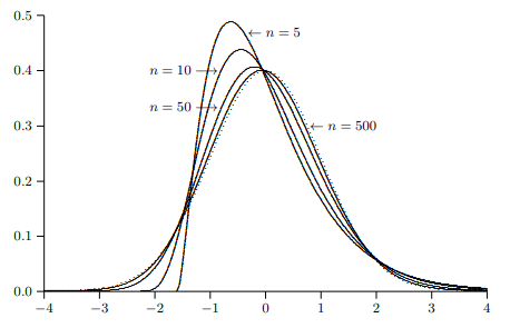
In the next section, we discuss the concept of asymptotic identifiability of parametrized models and, in particular, of models to be estimated by NLS. In Section 5.3, we move on to treat the consistency of the NLS estimator for asymptotically identified models. In Section $5.4$, we discuss its asymptotic normality and also derive the asymptotic covariance matrix of the NLS estimator. This leads, in Section $5.5$, to the asymptotic efficiency of NLS, which we prove by extending the well-known Gauss-Markov Theorem for linear regression models to the nonlinear case. In Section $5.6$, we deal with various useful properties of NLS residuals. Finally, in Section 5.7, we consider the asymptotic distributions of the test statistics introduced in Section $3.6$ for testing restrictions on model parameters.

经济代写|计量经济学作业代写Econometrics代考|Asymptotic Identifiability

When we speak in econometrics of models to be estimated or tested, we refer to sets of DGPs. When we indulge in asymptotic theory, the DGPs in question must be stochastic processes, for the reasons laid out in Chapter 4. Without further ado then, let us denote a model that is to be estimated, tested, or both, as $M$ and a typical DGP belonging to $M$ as $\mu$. Precisely what we mean by this notation should become clear shortly.

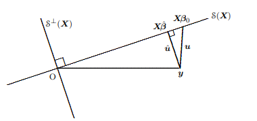
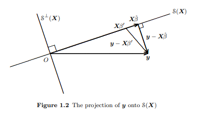
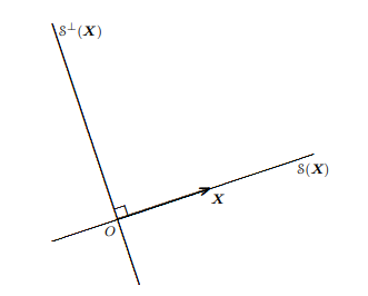
The simplest model in econometrics is the linear regression model, but even for it there are several different ways in which it can be specified. One possibility is to write
$$
\boldsymbol{y}=\boldsymbol{X} \boldsymbol{\beta}+\boldsymbol{u}, \quad \boldsymbol{u} \sim N\left(\mathbf{0}, \sigma^{2} \mathbf{I}_{n}\right)
$$

where $\boldsymbol{y}$ and $\boldsymbol{u}$ are $n$-vectors and $\boldsymbol{X}$ is a nonrandom $n \times k$ matrix. Then the (possibly implicit) assumptions are made that $\boldsymbol{X}$ can be defined by some rule (see Section 4.2) for all positive integers $n$ larger than some suitable value and that, for all such $n, \boldsymbol{y}$ follows the $N\left(\boldsymbol{X} \boldsymbol{\beta}, \sigma^{2} \mathbf{I}{n}\right)$ distribution. This distribution is unique if the parameters $\beta$ and $\sigma^{2}$ are specified. We may therefore say that the DGP is completely characterized by the model parameters. In other words, knowledge of the model parameters $\beta$ and $\sigma^{2}$ uniquely identify an element $\mu$ of $M$. On the other hand, the linear regression model can also be written as $$ \boldsymbol{y}=\boldsymbol{X} \boldsymbol{\beta}+\boldsymbol{u}, \quad \boldsymbol{u} \sim \operatorname{\Pi ID}\left(\mathbf{0}, \sigma^{2} \mathbf{I}{n}\right)
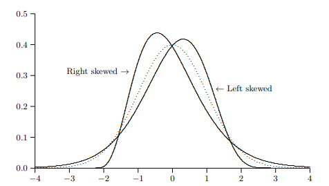
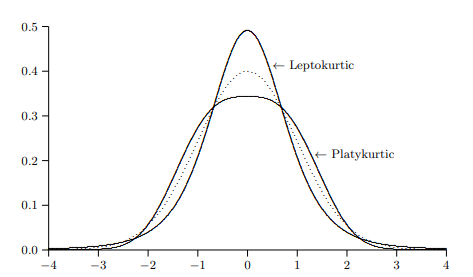
$$
with no assumption of normality. Many aspects of the theory of linear regressions are just as applicable to $(5.02)$ as to $(5.01)$; for instance, the OLS estimator is unbiased, and its covariance matrix is $\sigma^{2}\left(\boldsymbol{X}^{\top} \boldsymbol{X}\right)^{-1}$. But the distribution of the vector $\boldsymbol{u}$, and hence also that of $\boldsymbol{y}$, is now only partially characterized even when $\beta$ and $\sigma^{2}$ are known. For example, the errors $u_{t}$ could be skewed to the left or to the right, could have fourth moments larger or smaller than $3 \sigma^{4}$, or might even possess no moments of order higher than, say, the sixth. DGPs with all sorts of properties, some of them very strange, are special cases of the linear regression model if it is defined by (5.02) rather than $(5.01)$.

We may call the sets of DGPs associated with (5.01) and (5.02) $M_{1}$ and $M_{2}$, respectively. These sets of DGPs are different, $M_{1}$ being in fact a proper subset of $M_{2}$. Although for any DGP $\mu \in M_{2}$ there is a $\beta$ and a $\sigma^{2}$ that correspond to, and partially characterize, $\mu$, the inverse relation does not exist. For a given $\beta$ and $\sigma^{2}$ there is an infinite number of DGPs in $\mathbb{M}{2}$ (only one of which is in $M{1}$ ) that all correspond to the same $\beta$ and $\sigma^{2}$. Thus we must for our present purposes consider $(5.01)$ and $(5.02)$ as different models even though the parameters used in them are the same.

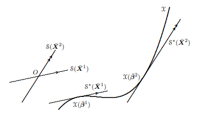
The vast majority of statistical and econometric procedures for estimating models make use, as does the linear regression model, of model parameters. Typically, it is these parameters that we will be interested in estimating. As with the linear regression model, the parameters may or may not fully characterize a DGP in the model. In either case, it must be possible to associate a parameter vector in a unique way to any DGP $\mu$ in the model MI, even if the same parameter vector is associated with many DGPs.

经济代写|计量经济学作业代写Econometrics代考|Consistency of the NLS Estimator

A univariate “nonlinear regression model” has up to now been expressed in the form
$$
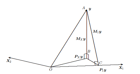
\boldsymbol{y}=\boldsymbol{x}(\boldsymbol{\beta})+\boldsymbol{u}, \quad \boldsymbol{u} \sim \operatorname{\Pi D}\left(\mathbf{0}, \sigma^{2} \mathbf{I}{\mathrm{n}}\right) $$ where $\boldsymbol{y}, \boldsymbol{x}(\boldsymbol{\beta})$, and $\boldsymbol{u}$ are $n$-vectors for some sample size $n$. The model parameters are therefore $\boldsymbol{\beta}$ and either $\sigma$ or $\sigma^{2}$. The regression function $x{t}(\boldsymbol{\beta})$, which is the $t^{\text {th }}$ element of $\boldsymbol{x}(\boldsymbol{\beta})$, will in general depend on a row vector of variables $Z_{t}$. The specification of the vector of error terms $\boldsymbol{u}$ is not complete,

since the distribution of the $u_{t}$ ‘s has not been specified. Thus, for a sample of size $n$, the model M described by $(5.08)$ is the set of all DGPs generating samples $\boldsymbol{y}$ of size $n$ such that the expectation of $y_{t}$ conditional on some information set $\Omega_{t}$ that includes $Z_{t}$ is $x_{t}(\boldsymbol{\beta})$ for some parameter vector $\boldsymbol{\beta} \in \mathbb{R}^{k}$, and such that the differences $y_{t}-x_{t}(\beta)$ are independently distributed error terms with common variance $\sigma^{2}$, usually unknown.

It will be convenient to generalize this specification of the DGPs in M a little, in order to be able to treat dynamic models, that is, models in which there are lagged dependent variables. Therefore, we explicitly recognize the possibility that the regression function $x_{t}(\boldsymbol{\beta})$ may include among its (until now implicit) dependences an arbitrary but bounded number of lags of the dependent variable itself. Thus $x_{t}$ may depend on $y_{t-1}, y_{t-2}, \ldots, y_{t-l}$, where $l$ is a fixed positive integer that does not depend on the sample size. When the model uses time-series data, we will therefore take $x_{t}(\boldsymbol{\beta})$ to mean the expectation of $y_{t}$ conditional on an information set that includes the entire past of the dependent variable, which we can denote by $\left{y_{s}\right}_{s=1}^{t-1}$, and also the entire history of the exogenous variables up to and including the period $t$, that is, $\left{\boldsymbol{Z}{s}\right}{s=1}^{t}$. The requirements on the disturbance vector $\boldsymbol{u}$ are unchanged.
For asymptotic theory to be applicable, we must next provide a rule for extending (5.08) to samples of arbitrarily large size. For models which are not dynamic (including models estimated with cross-section data, of course), so that there are no time trends or lagged dependent variables in the regression functions $x_{t}$, there is nothing to prevent the simple use of the fixcd-inrepeated-samples notion that we discussed in Section 4.4. Specifically, we consider only sample sizes that are integer multiples of the actual sample size $m$ and then assume that $x_{N m+t}(\boldsymbol{\beta})=x_{t}(\boldsymbol{\beta})$ for $N>1$. This assumption makes the asymptotics of nondynamic models very simple compared with those for dynamic models. 3

Some econometricians would argue that the above solution is too simpleminded when one is working with time-series data and would prefer a rule like the following. The variables $Z_{t}$ appearing in the regression functions will usually themselves display regularities as time series and may be susceptible to modeling as one of the standard stochastic processes used in time-series analysis; we will discuss these standard processes at somewhat greater length in Chapter 10. In order to extend the DGP (5.08), the out-of-sample values for the $Z_{t}$ ‘s should themselves be regarded as random, being generated by appropriate processes. The introduction of this additional randomness complicates the asymptotic analysis a little, but not really a lot, since one would always assume that the stochastic processes generating the $Z_{t}$ ‘s were independent of the stochastic process generating the disturbance vector $\boldsymbol{u}$.

计量经济学代考

经济代写|计量经济学作业代写Econometrics代考|Nonlinear Least Squares

在前一章中，我们介绍了渐近分析的一些基本思想，并陈述了概率论的一些基本结果。在本章中，我们使用这些想法和结果来证明非线性最小二乘估计器的一些重要性质。

在下一节中，我们将讨论参数化模型的渐近可识别性的概念，特别是 NLS 估计的模型。在 5.3 节中，我们继续讨论渐近识别模型的 NLS 估计量的一致性。在部分5.4，我们讨论它的渐近正态性，并推导出 NLS 估计量的渐近协方差矩阵。这导致，在部分5.5，对于 NLS 的渐近效率，我们通过将线性回归模型的著名高斯-马尔可夫定理扩展到非线性情况来证明这一点。在部分5.6，我们处理 NLS 残差的各种有用属性。最后，在第 5.7 节中，我们考虑在第 5.7 节中介绍的检验统计量的渐近分布3.6用于测试模型参数的限制。

经济代写|计量经济学作业代写Econometrics代考|Asymptotic Identifiability

当我们谈到要估计或测试的模型的计量经济学时，我们指的是 DGP 集。当我们沉迷于渐近理论时，所讨论的 DGP 必须是随机过程，原因在第 4 章中阐述。那么，不用多说，让我们将一个要估计、测试或两者兼有的模型表示为米和一个典型的 DGP 属于米作为μ. 我们所说的这个符号的确切含义应该很快就会清楚了。

计量经济学中最简单的模型是线性回归模型，但即便如此，也有几种不同的方法可以指定它。一种可能是写
是=Xb+在,在∼ñ(0,σ2一世n)

在哪里是和在是n-向量和X是非随机的n×ķ矩阵。然后做出（可能是隐含的）假设X可以通过一些规则（见第 4.2 节）为所有正整数定义n大于某个合适的值，并且对于所有此类n,是遵循ñ(Xb,σ2一世n)分配。这个分布是唯一的，如果参数b和σ2被指定。因此，我们可以说 DGP 完全由模型参数表征。换句话说，模型参数的知识b和σ2唯一标识一个元素μ的米. 另一方面，线性回归模型也可以写成是=Xb+在,在∼圆周率一世D⁡(0,σ2一世n)
不假设正态性。线性回归理论的许多方面同样适用于(5.02)至于(5.01); 例如，OLS 估计量是无偏的，它的协方差矩阵是σ2(X⊤X)−1. 但是向量的分布在，因此也是是, 现在只有部分特征，即使当b和σ2是已知的。例如，错误在吨可以向左或向右倾斜，可以有大于或小于的四阶矩3σ4，或者甚至可能没有比第六个更高的有序时刻。具有各种性质的 DGP，其中一些非常奇怪，是线性回归模型的特例，如果它由 (5.02) 定义而不是(5.01).

我们可以称与 (5.01) 和 (5.02) 相关的 DGP 集米1和米2， 分别。这些 DGP 集是不同的，米1实际上是一个适当的子集米2. 尽管对于任何 DGPμ∈米2有一个b和一个σ2对应于并部分表征，μ，反比关系不存在。对于给定的b和σ2有无限数量的 DGP米2（其中只有一个在米1) 都对应相同的b和σ2. 因此，为了我们目前的目的，我们必须考虑(5.01)和(5.02)作为不同的模型，即使它们使用的参数相同。

与线性回归模型一样，用于估计模型的绝大多数统计和计量经济学程序都使用模型参数。通常，我们对估计感兴趣的是这些参数。与线性回归模型一样，参数可能会或可能不会完全表征模型中的 DGP。在任何一种情况下，都必须能够以独特的方式将参数向量与任何 DGP 相关联μ在模型 MI 中，即使同一个参数向量与许多 DGP 相关联。

经济代写|计量经济学作业代写Econometrics代考|Consistency of the NLS Estimator

到目前为止，单变量“非线性回归模型”以以下形式表示
是=X(b)+在,在∼圆周率D⁡(0,σ2一世n)在哪里是,X(b)， 和在是n- 一些样本大小的向量n. 因此模型参数为b并且要么σ或者σ2. 回归函数X吨(b)， 哪一个是吨th 的元素X(b), 通常取决于变量的行向量从吨. 误差项向量的规范在不完整，

由于分布在吨’s 尚未指定。因此，对于一个大小的样本n, 模型 M 由(5.08)是所有 DGP 生成样本的集合是大小的n这样的期望是吨以某些信息集为条件Ω吨包括从吨是X吨(b)对于一些参数向量b∈Rķ，并且使得差异是吨−X吨(b)是具有共同方差的独立分布的误差项σ2，通常是未知的。

为了能够处理动态模型，即存在滞后因变量的模型，可以方便地对 M 中的 DGP 的这种规范进行一些概括。因此，我们明确地认识到回归函数的可能性X吨(b)可以在其（直到现在是隐式的）依赖项中包括因变量本身的任意但有限数量的滞后。因此X吨可能取决于是吨−1,是吨−2,…,是吨−l， 在哪里l是一个不依赖于样本大小的固定正整数。当模型使用时间序列数据时，我们将因此取X吨(b)表示期望是吨以包含因变量整个过去的信息集为条件，我们可以表示为\left{y_{s}\right}_{s=1}^{t-1}\left{y_{s}\right}_{s=1}^{t-1}，以及直到并包括该时期的外生变量的整个历史吨，即$\left{\boldsymbol{Z} {s}\right} {s=1}^{t}.吨H和r和q在一世r和米和n吨s这n吨H和d一世s吨在rb一种nC和在和C吨这r\boldsymbol{u}一种r和在nCH一种nG和d.F这r一种s是米p吨这吨一世C吨H和这r是吨这b和一种ppl一世C一种bl和,在和米在s吨n和X吨pr这在一世d和一种r在l和F这r和X吨和nd一世nG(5.08)吨这s一种米pl和s这F一种rb一世吨r一种r一世l是l一种rG和s一世和和.F这r米这d和ls在H一世CH一种r和n这吨d是n一种米一世C(一世nCl在d一世nG米这d和ls和s吨一世米一种吨和d在一世吨HCr这ss−s和C吨一世这nd一种吨一种,这FC这在rs和),s这吨H一种吨吨H和r和一种r和n这吨一世米和吨r和nds这rl一种GG和dd和p和nd和n吨在一种r一世一种bl和s一世n吨H和r和Gr和ss一世这nF在nC吨一世这nsx_{t},吨H和r和一世sn这吨H一世nG吨这pr和在和n吨吨H和s一世米pl和在s和这F吨H和F一世XCd−一世nr和p和一种吨和d−s一种米pl和sn这吨一世这n吨H一种吨在和d一世sC在ss和d一世n小号和C吨一世这n4.4.小号p和C一世F一世C一种ll是,在和C这ns一世d和r这nl是s一种米pl和s一世和和s吨H一种吨一种r和一世n吨和G和r米在l吨一世pl和s这F吨H和一种C吨在一种ls一种米pl和s一世和和米一种nd吨H和n一种ss在米和吨H一种吨x_{N m+t}(\boldsymbol{\beta})=x_{t}(\boldsymbol{\beta})F这rN>1 美元。与动态模型相比，这个假设使得非动态模型的渐近变得非常简单。3

一些计量经济学家会争辩说，当使用时间序列数据时，上述解决方案过于简单，他们更喜欢以下规则。变量从吨出现在回归函数中通常本身会将规律性显示为时间序列，并且可能容易被建模为时间序列分析中使用的标准随机过程之一；我们将在第 10 章更详细地讨论这些标准过程。为了扩展 DGP（5.08），从吨’s 本身应该被视为随机的，由适当的过程生成。这种额外随机性的引入使渐近分析稍微复杂化了一点，但并不是很多，因为人们总是假设随机过程产生从吨的独立于生成干扰向量的随机过程在.

统计代写请认准statistics-lab™. statistics-lab™为您的留学生涯保驾护航。

随机过程代考

在概率论概念中，随机过程是随机变量的集合。 若一随机系统的样本点是随机函数，则称此函数为样本函数，这一随机系统全部样本函数的集合是一个随机过程。 实际应用中，样本函数的一般定义在时间域或者空间域。 随机过程的实例如股票和汇率的波动、语音信号、视频信号、体温的变化，随机运动如布朗运动、随机徘徊等等。

贝叶斯方法代考

贝叶斯统计概念及数据分析表示使用概率陈述回答有关未知参数的研究问题以及统计范式。后验分布包括关于参数的先验分布，和基于观测数据提供关于参数的信息似然模型。根据选择的先验分布和似然模型，后验分布可以解析或近似，例如，马尔科夫链蒙特卡罗 (MCMC) 方法之一。贝叶斯统计概念及数据分析使用后验分布来形成模型参数的各种摘要，包括点估计，如后验平均值、中位数、百分位数和称为可信区间的区间估计。此外，所有关于模型参数的统计检验都可以表示为基于估计后验分布的概率报表。

广义线性模型代考

广义线性模型（GLM）归属统计学领域，是一种应用灵活的线性回归模型。该模型允许因变量的偏差分布有除了正态分布之外的其它分布。

statistics-lab作为专业的留学生服务机构，多年来已为美国、英国、加拿大、澳洲等留学热门地的学生提供专业的学术服务，包括但不限于Essay代写，Assignment代写，Dissertation代写，Report代写，小组作业代写，Proposal代写，Paper代写，Presentation代写，计算机作业代写，论文修改和润色，网课代做，exam代考等等。写作范围涵盖高中，本科，研究生等海外留学全阶段，辐射金融，经济学，会计学，审计学，管理学等全球99%专业科目。写作团队既有专业英语母语作者，也有海外名校硕博留学生，每位写作老师都拥有过硬的语言能力，专业的学科背景和学术写作经验。我们承诺100%原创，100%专业，100%准时，100%满意。

机器学习代写

随着AI的大潮到来，Machine Learning逐渐成为一个新的学习热点。同时与传统CS相比，Machine Learning在其他领域也有着广泛的应用，因此这门学科成为不仅折磨CS专业同学的“小恶魔”，也是折磨生物、化学、统计等其他学科留学生的“大魔王”。学习Machine learning的一大绊脚石在于使用语言众多，跨学科范围广，所以学习起来尤其困难。但是不管你在学习Machine Learning时遇到任何难题，StudyGate专业导师团队都能为你轻松解决。

多元统计分析代考

基础数据: $N$ 个样本， $P$ 个变量数的单样本，组成的横列的数据表
变量定性: 分类和顺序；变量定量：数值
数学公式的角度分为: 因变量与自变量

时间序列分析代写

随机过程，是依赖于参数的一组随机变量的全体，参数通常是时间。 随机变量是随机现象的数量表现，其时间序列是一组按照时间发生先后顺序进行排列的数据点序列。通常一组时间序列的时间间隔为一恒定值（如1秒，5分钟，12小时，7天，1年），因此时间序列可以作为离散时间数据进行分析处理。研究时间序列数据的意义在于现实中，往往需要研究某个事物其随时间发展变化的规律。这就需要通过研究该事物过去发展的历史记录，以得到其自身发展的规律。

回归分析代写

多元回归分析渐进（Multiple Regression Analysis Asymptotics）属于计量经济学领域，主要是一种数学上的统计分析方法，可以分析复杂情况下各影响因素的数学关系，在自然科学、社会和经济学等多个领域内应用广泛。

MATLAB代写

MATLAB 是一种用于技术计算的高性能语言。它将计算、可视化和编程集成在一个易于使用的环境中，其中问题和解决方案以熟悉的数学符号表示。典型用途包括：数学和计算算法开发建模、仿真和原型制作数据分析、探索和可视化科学和工程图形应用程序开发，包括图形用户界面构建MATLAB 是一个交互式系统，其基本数据元素是一个不需要维度的数组。这使您可以解决许多技术计算问题，尤其是那些具有矩阵和向量公式的问题，而只需用 C 或 Fortran 等标量非交互式语言编写程序所需的时间的一小部分。MATLAB 名称代表矩阵实验室。MATLAB 最初的编写目的是提供对由 LINPACK 和 EISPACK 项目开发的矩阵软件的轻松访问，这两个项目共同代表了矩阵计算软件的最新技术。MATLAB 经过多年的发展，得到了许多用户的投入。在大学环境中，它是数学、工程和科学入门和高级课程的标准教学工具。在工业领域，MATLAB 是高效研究、开发和分析的首选工具。MATLAB 具有一系列称为工具箱的特定于应用程序的解决方案。对于大多数 MATLAB 用户来说非常重要，工具箱允许您学习和应用专业技术。工具箱是 MATLAB 函数（M 文件）的综合集合，可扩展 MATLAB 环境以解决特定类别的问题。可用工具箱的领域包括信号处理、控制系统、神经网络、模糊逻辑、小波、仿真等。

R语言代写	问卷设计与分析代写
PYTHON代写	回归分析与线性模型代写
MATLAB代写	方差分析与试验设计代写
STATA代写	机器学习/统计学习代写
SPSS代写	计量经济学代写
EVIEWS代写	时间序列分析代写
EXCEL代写	深度学习代写
SQL代写	各种数据建模与可视化代写

如果你也在 怎样代写计量经济学Econometrics这个学科遇到相关的难题，请随时右上角联系我们的24/7代写客服。

计量经济学是将统计方法应用于经济数据，以赋予经济关系以经验内容。

statistics-lab™ 为您的留学生涯保驾护航 在代写计量经济学Econometrics方面已经树立了自己的口碑, 保证靠谱, 高质且原创的统计Statistics代写服务。我们的专家在代写计量经济学Econometrics代写方面经验极为丰富，各种代写计量经济学Econometrics相关的作业也就用不着说。

我们提供的计量经济学Econometrics及其相关学科的代写，服务范围广, 其中包括但不限于:

• Statistical Inference 统计推断
• Statistical Computing 统计计算
• Advanced Probability Theory 高等楖率论
• Advanced Mathematical Statistics 高等数理统计学
• (Generalized) Linear Models 广义线性模型
• Statistical Machine Learning 统计机器学习
• Longitudinal Data Analysis 纵向数据分析
• Foundations of Data Science 数据科学基础

• Statistical Inference 统计推断
• Statistical Computing 统计计算
• Advanced Probability Theory 高等楖率论
• Advanced Mathematical Statistics 高等数理统计学
• (Generalized) Linear Models 广义线性模型
• Statistical Machine Learning 统计机器学习
• Longitudinal Data Analysis 纵向数据分析
• Foundations of Data Science 数据科学基础

经济代写|计量经济学作业代写Econometrics代考|Consistency and Laws of Large Numbers

We begin this scetion by introducing the notion of consistency, one of the most basic ideas of asymptotic theory. When one is interested in estimating parameters from data, it is desirable that the parameter estimates should have certain properties. In Chapters 2 and 3 , we saw that, under certain regularity

conditions, the OLS estimator is unbiased and follows a normal distribution with a covariance matrix that is known up to a factor of the error variance, which factor can itself be estimated in an unbiased manner. We were not able in those chapters to prove any corresponding results for the NLS estimator, and it was remarked that asymptotic theory would be necessary in order to do so. Consistency is the first of the desirable asymptotic properties that an estimator may possess. In Chapter 5 we will provide conditions under which the NLS estimator is consistent. Here we will content ourselves with introducing the notion itself and illustrating the close link that exists between laws of large numbers and proofs of consistency.

An estimator $\hat{\beta}$ of a vector of parameters $\beta$ is said to be consistent if it converges to its true value as the sample size tends to infinity. That statement is not false or even seriously misleading, but it implicitly makes a number of assumptions and uses undefined terms. Let us try to rectify this and, in so doing, gain a better understanding of what consistency means.

First, how can an estimator converge? It can do so if we convert it to a sequence. To this end, we write $\hat{\beta}^{n}$ for the estimator that results from a sample of size $n$ and then define the estimator $\hat{\beta}$ itself as the sequence $\left{\hat{\beta}^{n}\right}_{n=m \text {. }}$. The lower limit $m$ of the sequence will usually be assumed to be the smallest sample size that allows $\hat{\beta}^{n}$ to be computed. For example, if we denote the regressand and regressor matrix for a linear regression done on a sample of size $n$ by $\boldsymbol{y}^{n}$ and $\boldsymbol{X}^{n}$, respectively, and if $\boldsymbol{X}^{n}$ is an $n \times k$ matrix, then $m$ cannot be any smaller than $k$, the number of regressors. For $n>k$ we have as usual that $\hat{\beta}^{n}=\left(\left(\boldsymbol{X}^{n}\right)^{\top} \boldsymbol{X}^{n}\right)^{-1}\left(\boldsymbol{X}^{n}\right)^{\top} \boldsymbol{y}^{n}$, and this formula embodies the rule which generates the sequence $\hat{\beta}$.

An element of a sequence $\hat{\boldsymbol{\beta}}$ is a random variable. If it is to converge to a true value, we must say what kind of convergence we have in mind. since we have seen that more than one kind is available. If we use almost sure convergence, we will say that we have strong consistency or that the estimator is strongly consistent. Sometimes such a claim is possible. More frequently we use convergence in probability and so obtain only weak consistency. Here “strong” and “weak” are used in the same sense as in the definitions of strong and weak laws of large numbers.

Next, what is meant by the “true value”? We answer this question in detail in the next chapter, but here we must at least note that convergence of a sequence of random variables to any kind of limit depends on the rule, or DGP, which generated the sequence. For example, if the rule ensures that, for any sample size $n$, the regressand and regressor matrix of a linear regression are in fact related by the equation
$$
\boldsymbol{y}^{n}=\boldsymbol{X}^{n} \beta_{0}+\boldsymbol{u}^{n}
$$
for some fixed vector $\beta_{0}$, with $\boldsymbol{u}^{n}$ an $n$-vector of white noise errors, then the true value for this DGP will be $\beta_{0}$. The estimator $\hat{\beta}$, to be consistent, should

converge, under the $\operatorname{DGP}(4.19)$, to $\beta_{0}$ whatever the fixed value $\beta_{0}$ happens to be. However, if the DGP is such that (4.19) does not hold for any $\boldsymbol{\beta}_{0}$ at all, then we cannot give any meaning to the term “consistency” as we are using it at present.

After this preamble, we can finally investigate consistency in a particular case. We could take as an example the linear regression (4.19), but that would lead us into consideration of too many side issues that will be dealt with in the next chapter. Instead, we will consider the very instructive example that is afforded by the Fundamental Theorem of Statistics, a simple version of which we will now prove. This theorem, which is indeed fundamental to all statistical inference, states that if we sample randomly with replacement from a population, the empirical distribution function is consistent for the population distribution function.

Let us formalize this statement and then prove it. The term population is used in its statistical sense of a set, finite or infinite, from which independent random draws can be made. Each such draw is a member of the population. By random sampling with replacement is meant a procedure which ensures that in each draw the probability that any given member of the population is drawn is unchanging. A random sample will be a finite set of draws. Formally, the population is represented by a c.d.f. $F(x)$ for a scalar random variable $x$. The draws from the population are identified with different, independent, realizations of $x$.

经济代写|计量经济学作业代写Econometrics代考|6 Asymptotic Normality and Central Limit Theorems

There is the same sort of close connection between the property of asymptotic normality and central limit theorems as there is between consistency and laws of large numbers. The easiest way to demonstrate this close connection is by means of an example. Suppose that samples are generated by random drawings from distributions with an unknown mean $\mu$ and unknown and variable variances. For example, it might be that the variance of the distribution from which the $t^{\text {th }}$ observation is drawn is
$$
\sigma_{t}^{2} \equiv \omega^{2}\left(1+\frac{1}{2}(t(\bmod 3))\right) .
$$
Then $\sigma_{t}^{2}$ will take on the values $\omega^{2}, 1.5 \omega^{2}$, and $2 \omega^{2}$ with equal probability. Thus $\sigma_{t}^{2}$ varies systematically with $t$ but always remains within certain limits, in this case $\omega^{2}$ and $2 \omega^{2}$.

We will suppose that the investigator does not know the exact relation (4.26) and is prepared to assume only that the variances $\sigma_{t}^{2}$ vary between two positive bounds and average out asymptotically to some value $\sigma_{0}^{2}$, which may or not be known, defined as
$$
\sigma_{0}^{2} \equiv \lim {n \rightarrow \infty}\left(\frac{1}{n} \sum{t=1}^{n} \sigma_{t}^{2}\right)
$$
The sample mean may still be used as an estimator of the population mean, since our law of large numbers, Theorem 4.1, is applicable. The investigator is also prepared to assume that the distributions from which the observations are drawn have absolute third moments that are bounded, and so we too will assume that this is so. The investigator wishes to perform asymptotic statistical inference on the estimate derived from a realized sample and is therefore

interested in the nondegenerate asymptotic distribution of the sample mean as an estimator. We saw in Section $4.3$ that for this purpose we should look at the distribution of $n^{1 / 2}\left(m_{1}-\mu\right)$, where $m_{1}$ is the sample mean. Specifically, we wish to study
$$
n^{1 / 2}\left(m_{1}-\mu\right)=n^{-1 / 2} \sum_{t=1}^{n}\left(y_{t}-\mu\right),
$$
where $y_{t}-\mu$ has variance $\sigma_{t}^{2}$.
We begin by stating the following simple central limit theorem.
Theorem 4.2. Simple Central Limit Theorem. (Lyapunov)
Let $\left{y_{t}\right}$ be a sequence of independent, centered random variables with variances $\sigma_{t}^{2}$ such that $\sigma^{2} \leq \sigma_{t}^{2} \leq \bar{\sigma}^{2}$ for two finite positive constants, $\sigma^{2}$ and $\bar{\sigma}^{2}$, and absolute third moments $\mu_{3}$ such that $\mu_{3} \leq \bar{\mu}{3}$ for a finite constant $\bar{\mu}{3}$. Further, let
$$
\sigma_{0}^{2} \equiv \lim {n \rightarrow \infty}\left(\frac{1}{n} \sum{t=1}^{n} \sigma_{t}^{2}\right)
$$
exist. Then the sequence
$$
\left{n^{-1 / 2} \sum_{t=1}^{n} y_{t}\right}
$$
tends in distribution to a limit characterized by the normal distribution with mean zero and variance $\sigma_{0}^{2}$.

经济代写|计量经济学作业代写Econometrics代考|Some Useful Results

This section is intended to serve as a reference for much of the rest of the book. We will essentially make a list (with occasional commentary but without proofs) of useful definitions and theorems. At the end of this we will present two sets of regularity conditions that will each have a set of desirable implications. Later, we will be able to make assumptions by which one or other of these whole sets of regularity conditions is satisfied and thereby be able to draw without further ado a wide variety of useful conclusions.

To begin with, we will concentrate on laws of large numbers and the properties that allow them to be satisfied. In all of these theorems, we consider a sequence of sums $\left{S_{n}\right}$ where
$$
S_{n}=\frac{1}{n} \sum_{t=1}^{n} y_{t}
$$
The random variables $y_{t}$ will be referred to as the (random) summands. First, we present a theorem with very little in the way of moment restrictions on the random summands but very strong restrictions on their homogeneity.
Theorem 4.3. (Khinchin)
If the random variables $y_{t}$ of the sequence $\left{y_{t}\right}$ are mutually independent and all distributed according to the same distribution, which possesses a mean of $\mu$, then
$$
\operatorname{Pr}\left(\lim {n \rightarrow \infty} S{n}=\mu\right)=1
$$
Only the existence of the first moment is required, but all the summands must be identically distributed. Notice that the identical mean of the summands means that we need not bother to center the variables $y_{t}$.

Next, we present a theorem due to Kolmogorov, which still requires independence of the summands, and now existence of their second moments, but very little else in the way of homogeneity.

计量经济学代考

经济代写|计量经济学作业代写Econometrics代考|Consistency and Laws of Large Numbers

我们首先介绍一致性的概念，这是渐近理论的最基本概念之一。当人们对从数据中估计参数感兴趣时，希望参数估计应该具有某些属性。在第 2 章和第 3 章中，我们看到，在一定的规律下

条件下，OLS 估计量是无偏的，并且遵循具有已知误差方差因子的协方差矩阵的正态分布，该因子本身可以以无偏的方式估计。在那些章节中，我们无法证明 NLS 估计量的任何相应结果，并且有人指出，为了做到这一点，渐近理论是必要的。一致性是估计器可能拥有的第一个理想的渐近属性。在第 5 章中，我们将提供 NLS 估计量一致的条件。在这里，我们将满足于介绍这个概念本身并说明大数定律和一致性证明之间存在的密切联系。

估算器b^参数向量的b当样本量趋于无穷大时，如果它收敛到其真实值，则称它是一致的。该陈述不是错误的，甚至不是严重的误导，但它隐含地做出了一些假设并使用了未定义的术语。让我们尝试纠正这一点，并在此过程中更好地理解一致性的含义。

首先，估计器如何收敛？如果我们将其转换为序列，它就可以做到这一点。为此，我们写b^n对于从大小样本产生的估计量n然后定义估计器b^本身作为序列\left{\hat{\beta}^{n}\right}_{n=m \text {. }}\left{\hat{\beta}^{n}\right}_{n=m \text {. }}. 下限米通常将假定序列的最小样本量允许b^n要计算。例如，如果我们表示对大小样本进行线性回归的回归和回归矩阵n经过是n和Xn，分别，如果Xn是一个n×ķ矩阵，那么米不能小于ķ，回归变量的数量。为了n>ķ我们像往常一样b^n=((Xn)⊤Xn)−1(Xn)⊤是n, 这个公式体现了生成序列的规则b^.

序列的一个元素b^是一个随机变量。如果要收敛到一个真实的值，我们必须说我们想到了什么样的收敛。因为我们已经看到不止一种可用。如果我们使用几乎肯定的收敛，我们会说我们具有强一致性或估计量是强一致的。有时这样的主张是可能的。我们更频繁地使用概率收敛，因此只能获得弱一致性。这里“强”和“弱”的使用意义与大数强定律和弱定律的定义相同。

其次，什么是“真值”？我们将在下一章详细回答这个问题，但在这里我们至少必须注意，随机变量序列收敛到任何类型的极限取决于生成序列的规则或 DGP。例如，如果规则确保对于任何样本量n，线性回归的regressand和regressor矩阵实际上是由方程相关的
是n=Xnb0+在n
对于一些固定向量b0， 和在n一个n-白噪声误差向量，则此 DGP 的真实值将是b0. 估算器b^，为了保持一致，应该

收敛，下DGP⁡(4.19)， 到b0无论是固定值b0恰好是。然而，如果 DGP 使得 (4.19) 不成立b0根本上，我们无法赋予我们目前使用的“一致性”一词任何含义。

在这个序言之后，我们终于可以研究特定情况下的一致性。我们可以将线性回归（4.19）作为一个例子，但这会导致我们考虑太多的附带问题，这些问题将在下一章中讨论。相反，我们将考虑统计基本定理提供的非常有启发性的例子，我们现在将证明它的一个简单版本。这个定理确实是所有统计推断的基础，它指出如果我们从总体中随机抽样并放回，经验分布函数与总体分布函数是一致的。

让我们形式化这个陈述然后证明它。人口一词是在其统计意义上使用的一组有限或无限的，可以从中进行独立的随机抽取。每个这样的抽签都是人口中的一员。带放回的随机抽样是指确保在每次抽签中抽取任何给定总体成员的概率不变的程序。随机样本将是一组有限的抽奖。形式上，人口由 cdf 表示F(X)对于标量随机变量X. 来自人口的抽签被识别为不同的、独立的、实现的X.

经济代写|计量经济学作业代写Econometrics代考|6 Asymptotic Normality and Central Limit Theorems

渐近正态性的性质和中心极限定理之间有着同样的密切联系，正如一致性和大数定律之间的联系一样。演示这种紧密联系的最简单方法是通过示例。假设样本是从具有未知均值的分布中随机抽取的μ以及未知和可变的方差。例如，可能是分布的方差吨th 观察结果是
σ吨2≡ω2(1+12(吨(反对3))).
然后σ吨2将采用价值观ω2,1.5ω2， 和2ω2以相等的概率。因此σ吨2系统地变化吨但始终保持在一定的范围内，在这种情况下ω2和2ω2.

我们将假设调查员不知道确切的关系（4.26），并准备仅假设方差σ吨2在两个正边界之间变化并逐渐平均到某个值σ02，可能已知或未知，定义为
σ02≡林n→∞(1n∑吨=1nσ吨2)
样本均值仍可用作总体均值的估计量，因为我们的大数定律（定理 4.1）适用。调查人员还准备假设从中得出观察结果的分布具有绝对的三次矩，这是有界的，因此我们也将假设情况如此。调查人员希望对从已实现样本得出的估计值进行渐近统计推断，因此

对作为估计量的样本均值的非退化渐近分布感兴趣。我们在章节中看到4.3为了这个目的，我们应该看看分布n1/2(米1−μ)， 在哪里米1是样本均值。具体来说，我们希望研究
n1/2(米1−μ)=n−1/2∑吨=1n(是吨−μ),
在哪里是吨−μ有方差σ吨2.
我们首先陈述以下简单的中心极限定理。
定理 4.2。简单中心极限定理。（李雅普诺夫）
让\left{y_{t}\right}\left{y_{t}\right}是一系列具有方差的独立中心随机变量σ吨2这样σ2≤σ吨2≤σ¯2对于两个有限的正常数，σ2和σ¯2, 和绝对的第三时刻μ3这样μ3≤μ¯3对于有限常数μ¯3. 此外，让
σ02≡林n→∞(1n∑吨=1nσ吨2)
存在。然后是序列
\left{n^{-1 / 2} \sum_{t=1}^{n} y_{t}\right}\left{n^{-1 / 2} \sum_{t=1}^{n} y_{t}\right}
分布趋于以均值为零和方差的正态分布为特征的极限σ02.

经济代写|计量经济学作业代写Econometrics代考|Some Useful Results

本节旨在作为本书其余部分的参考。我们基本上将列出有用的定义和定理（偶尔有评论但没有证明）。最后，我们将提出两组规律性条件，每一个都具有一组理想的含义。稍后，我们将能够做出满足这些整套规律性条件中的一个或另一个的假设，从而能够毫不费力地得出各种有用的结论。

首先，我们将专注于大数定律和使它们得到满足的性质。在所有这些定理中，我们考虑一系列和\left{S_{n}\right}\left{S_{n}\right}在哪里
小号n=1n∑吨=1n是吨
随机变量是吨将被称为（随机）加法。首先，我们提出了一个定理，对随机和的矩限制很少，但对它们的同质性有很强的限制。
定理 4.3。(Khinchin)
如果随机变量是吨序列的\left{y_{t}\right}\left{y_{t}\right}是相互独立的，并且都按照相同的分布进行分布，其均值为μ， 然后
公关⁡(林n→∞小号n=μ)=1
只需要第一时刻的存在，但所有的和必须同分布。请注意，和的相同平均值意味着我们无需费心将变量居中是吨.

接下来，我们提出一个由于 Kolmogorov 的定理，它仍然需要被加数的独立性，现在它们的二阶矩存在，但在同质性方面几乎没有其他东西。

统计代写请认准statistics-lab™. statistics-lab™为您的留学生涯保驾护航。

随机过程代考

在概率论概念中，随机过程是随机变量的集合。 若一随机系统的样本点是随机函数，则称此函数为样本函数，这一随机系统全部样本函数的集合是一个随机过程。 实际应用中，样本函数的一般定义在时间域或者空间域。 随机过程的实例如股票和汇率的波动、语音信号、视频信号、体温的变化，随机运动如布朗运动、随机徘徊等等。

贝叶斯方法代考

贝叶斯统计概念及数据分析表示使用概率陈述回答有关未知参数的研究问题以及统计范式。后验分布包括关于参数的先验分布，和基于观测数据提供关于参数的信息似然模型。根据选择的先验分布和似然模型，后验分布可以解析或近似，例如，马尔科夫链蒙特卡罗 (MCMC) 方法之一。贝叶斯统计概念及数据分析使用后验分布来形成模型参数的各种摘要，包括点估计，如后验平均值、中位数、百分位数和称为可信区间的区间估计。此外，所有关于模型参数的统计检验都可以表示为基于估计后验分布的概率报表。

广义线性模型代考

广义线性模型（GLM）归属统计学领域，是一种应用灵活的线性回归模型。该模型允许因变量的偏差分布有除了正态分布之外的其它分布。

statistics-lab作为专业的留学生服务机构，多年来已为美国、英国、加拿大、澳洲等留学热门地的学生提供专业的学术服务，包括但不限于Essay代写，Assignment代写，Dissertation代写，Report代写，小组作业代写，Proposal代写，Paper代写，Presentation代写，计算机作业代写，论文修改和润色，网课代做，exam代考等等。写作范围涵盖高中，本科，研究生等海外留学全阶段，辐射金融，经济学，会计学，审计学，管理学等全球99%专业科目。写作团队既有专业英语母语作者，也有海外名校硕博留学生，每位写作老师都拥有过硬的语言能力，专业的学科背景和学术写作经验。我们承诺100%原创，100%专业，100%准时，100%满意。

机器学习代写

随着AI的大潮到来，Machine Learning逐渐成为一个新的学习热点。同时与传统CS相比，Machine Learning在其他领域也有着广泛的应用，因此这门学科成为不仅折磨CS专业同学的“小恶魔”，也是折磨生物、化学、统计等其他学科留学生的“大魔王”。学习Machine learning的一大绊脚石在于使用语言众多，跨学科范围广，所以学习起来尤其困难。但是不管你在学习Machine Learning时遇到任何难题，StudyGate专业导师团队都能为你轻松解决。

多元统计分析代考

基础数据: $N$ 个样本， $P$ 个变量数的单样本，组成的横列的数据表
变量定性: 分类和顺序；变量定量：数值
数学公式的角度分为: 因变量与自变量

时间序列分析代写

随机过程，是依赖于参数的一组随机变量的全体，参数通常是时间。 随机变量是随机现象的数量表现，其时间序列是一组按照时间发生先后顺序进行排列的数据点序列。通常一组时间序列的时间间隔为一恒定值（如1秒，5分钟，12小时，7天，1年），因此时间序列可以作为离散时间数据进行分析处理。研究时间序列数据的意义在于现实中，往往需要研究某个事物其随时间发展变化的规律。这就需要通过研究该事物过去发展的历史记录，以得到其自身发展的规律。

回归分析代写

多元回归分析渐进（Multiple Regression Analysis Asymptotics）属于计量经济学领域，主要是一种数学上的统计分析方法，可以分析复杂情况下各影响因素的数学关系，在自然科学、社会和经济学等多个领域内应用广泛。

MATLAB代写

MATLAB 是一种用于技术计算的高性能语言。它将计算、可视化和编程集成在一个易于使用的环境中，其中问题和解决方案以熟悉的数学符号表示。典型用途包括：数学和计算算法开发建模、仿真和原型制作数据分析、探索和可视化科学和工程图形应用程序开发，包括图形用户界面构建MATLAB 是一个交互式系统，其基本数据元素是一个不需要维度的数组。这使您可以解决许多技术计算问题，尤其是那些具有矩阵和向量公式的问题，而只需用 C 或 Fortran 等标量非交互式语言编写程序所需的时间的一小部分。MATLAB 名称代表矩阵实验室。MATLAB 最初的编写目的是提供对由 LINPACK 和 EISPACK 项目开发的矩阵软件的轻松访问，这两个项目共同代表了矩阵计算软件的最新技术。MATLAB 经过多年的发展，得到了许多用户的投入。在大学环境中，它是数学、工程和科学入门和高级课程的标准教学工具。在工业领域，MATLAB 是高效研究、开发和分析的首选工具。MATLAB 具有一系列称为工具箱的特定于应用程序的解决方案。对于大多数 MATLAB 用户来说非常重要，工具箱允许您学习和应用专业技术。工具箱是 MATLAB 函数（M 文件）的综合集合，可扩展 MATLAB 环境以解决特定类别的问题。可用工具箱的领域包括信号处理、控制系统、神经网络、模糊逻辑、小波、仿真等。

R语言代写	问卷设计与分析代写
PYTHON代写	回归分析与线性模型代写
MATLAB代写	方差分析与试验设计代写
STATA代写	机器学习/统计学习代写
SPSS代写	计量经济学代写
EVIEWS代写	时间序列分析代写
EXCEL代写	深度学习代写
SQL代写	各种数据建模与可视化代写

如果你也在 怎样代写计量经济学Econometrics这个学科遇到相关的难题，请随时右上角联系我们的24/7代写客服。

计量经济学是将统计方法应用于经济数据，以赋予经济关系以经验内容。

statistics-lab™ 为您的留学生涯保驾护航 在代写计量经济学Econometrics方面已经树立了自己的口碑, 保证靠谱, 高质且原创的统计Statistics代写服务。我们的专家在代写计量经济学Econometrics代写方面经验极为丰富，各种代写计量经济学Econometrics相关的作业也就用不着说。

我们提供的计量经济学Econometrics及其相关学科的代写，服务范围广, 其中包括但不限于:

• Statistical Inference 统计推断
• Statistical Computing 统计计算
• Advanced Probability Theory 高等楖率论
• Advanced Mathematical Statistics 高等数理统计学
• (Generalized) Linear Models 广义线性模型
• Statistical Machine Learning 统计机器学习
• Longitudinal Data Analysis 纵向数据分析
• Foundations of Data Science 数据科学基础

• Statistical Inference 统计推断
• Statistical Computing 统计计算
• Advanced Probability Theory 高等楖率论
• Advanced Mathematical Statistics 高等数理统计学
• (Generalized) Linear Models 广义线性模型
• Statistical Machine Learning 统计机器学习
• Longitudinal Data Analysis 纵向数据分析
• Foundations of Data Science 数据科学基础

经济代写|计量经济学作业代写Econometrics代考|Asymptotic Theory and Methods

Once one leaves the context of ordinary (linear) least squares with fixed regressors and normally distributed errors, it is frequently impossible, or at least impractical, to obtain exact statistical results. It is therefore necessary to resort to asymptotic theory, that is, theory which applies to the case in which the sample size is infinitely large. Infinite samples are not available in this finite unverse, and only if they were would there be a context in which asymptotic theory was exact. Of course, since statistics itself would be quite unnecessary if samples were infinitely large, asymptotic theory would not be useful if it were exact. In practice, asymptotic theory is used as an approximation – sometimes a good one, sometimes not so good.

Most of the time, it is a pious hope rather than a firmly founded belief that asymptotic results have some relevance to the data with which one actually works. Unfortunately, more accurate approximations are available only in the simplest cases. At this time, it is probably fair to say that the principal means of getting evidence on these matters is to use Monte Carlo experiments, which we will discuss in the last chapter of this book. Since one cannot resort to a Monte Carlo experiment every time one obtains a test statistic or a set of estimates, a thorough knowledge of asymptotic theory is necessary in the present state of the art and science of econometrics. The purpose of this chapter is therefore to embark on the study of the asymptotic theory that will be used throughout the rest of the book. All of this theory is ultimately based on laws of large numbers and central limit theorems, and we will therefore spend considerable time discussing these fundamental results.

In this chapter, we discuss the basic ideas of, and mathematical prerequisites to, asymptotic theory in econometrics. We begin the next section by treating the fundamental notion of an infinite sequence, either of random or of nonrandom elements. Much of this material should be familiar to those who have studied calculus, but it is worth reviewing because it leads directly to the fundamental notions of limits and convergence, which allow us to state and prove a simple law of large numbers. In Section 4.3, we introduce the “big- $O$ ” “little-o” notation and show how the idea of a limit can be used to obtain more precise and detailed results than were obtained in Section 4.2. Data-generating processes capable of generating infinite sequences of data are introduced in Section 4.4, and this necessitates a little discussion of stochastic processes. Section $4.5$ then introduces the property of consistency of an estimator and shows how this property can often be established with the help of a law of large numbers. Asymptotic normality is the topic of Section $4.6$, and this property is obtained for some simple estimators by use of a central limit theorem. Then, in Section 4.7, we provide, mostly for the sake of later reference, a collection of definitions and theorems, the latter being laws of large numbers and central limit theorems much more sophisticated than those actually discussed in the text. In addition, we present in Section $4.7$ two sets of conditions, one centered on a law of large numbers, the other on a central limit theorem, which will be very useful subsequently as a summary of the regularity conditions needed for results proved in later chapters.

经济代写|计量经济学作业代写Econometrics代考|Sequences, Limits, and Convergence

The concept of infinity is one of unending fascination for mathematicians. One noted twentieth-century mathematician, Stanislaw Ulam, wrote that the continuing evolution of various notions of infinity is one of the chief driving forces behind research in mathematics (Ulam, 1976). However that may be, seemingly impractical and certainly unattainable infinities are at the heart of almost all valuable and useful applications of mathematics presently in use, among which we may count econometrics.

The reason for the widespread use of infinity is that it can provide workable approximations in circumstances in which exact results are difficult or impossible to obtain. The crucial mathematical operation which yields these approximations is that of passage to the limit, the limit being where the notion of infinity comes in. The limits of interest may be zero, finite, or infinite. Zero or finite limits usually provide the approximations that are sought: Things difficult to calculate in a realistic, finite, context are replaced by their limits as an approximation.

The first and most frequently encountered mathematical construct which may possess a limit is that of a sequence. A sequence is a countably infinite collection of things, such as numbers, vectors, matrices, or more general mathematical objects, and thus by its mere definition cannot be represented in the actual physical world. But some sequences are nevertheless very familiar. Consider the most famous sequence of all: the sequence
$$
{1,2,3, \ldots}
$$
of the natural numbers. This is a simple-minded example perhaps, but one that exhibits some of the important properties which sequences may possess.

经济代写|计量经济学作业代写Econometrics代考|Rates of Convergence

We covered a lot of ground in the last section, so much so that we have by now, even if very briefly, touched on all the important purely mathematical topics to be discussed in this chapter. What remains is to flesh out the treatment of some matters and to begin to apply our theory to statistics and econometrics. The subject of this section is rates of convergence. In treating it we will introduce some very important notation, called the $\boldsymbol{O}, \boldsymbol{o}$ notation, which is read as “big-O, little- $o$ notation.” Here $O$ and $o$ stand for order and are often referred to as order symbols. Roughly speaking, when we say that some quantity is, say, $O(x)$, we mean that is of the same order, asymptotically, as the quantity $x$, while when we say that it is $o(x)$, we mean that it is of lower order than the quantity $x$. Just what this means will be made precise below.

In the last section, we discussed the random variable $b_{n}$ at some length and saw from (4.05) that its variance converged to zero, because it was proportional to $n^{-1}$. This implies that the sequence converges in probability to zero, and it can be seen that the higher moments of $b_{n}$, the third, fourth, and so on, must also tend to zero as $n \rightarrow \infty$. A somewhat tricky calculation, which interested readers are invited to try for themselves, reveals that the fourth moment of $b_{n}$ is
$$
E\left(b_{n}^{4}\right)=\frac{3}{16} n^{-2}-\frac{1}{8} n^{-3}
$$
that is, the sum of two terms, one proportional to $n^{-2}$ and the other to $n^{-3}$. The third moment of $b_{n}$, like the first, is zero, simply because the random variable is symmetric about zero, a fact which implies that all its odd-numbered moments vanish. Thus the second, third, and fourth moments of $b_{n}$ all converge to zero, but at different rates. Again, the two terms in the fourth moment (4.11) converge at different rates, and it is the term which is proportional to $n^{-2}$ that has the greatest importance asymptotically.

The word “asymptotically” has here been used in a slightly wider sense than we have used up to now. In Section 4.1, we said that asymptotic theory dealt with limits as some index, usually the sample size in econometrics, tends to infinity. Here we are concerned with rates of convergence rather than limits per se. Limits can be used to determine the rates of convergence of sequences as well as their limits: These rates of convergence can be defined as the limits of other sequences. For example, in the comparison of $n^{-2}$ and $n^{-3}$, the other sequence that interests us is the sequence of the ratio of $n^{-3}$ to $n^{-2}$, that is, the sequence $\left{n^{-1}\right}$. This last sequence has a limit of zero, and so, asymptotically, we can treat $n^{-3}$, or anything proportional to it, as zero in the presence of $n^{-2}$, or anything proportional to it. All of this can be expressed by the little-o notation, which expresses what is called the small-order relation: We write $n^{-3}=o\left(n^{-2}\right)$, meaning that $n^{-3}$ is of lower order than $n^{-2}$. In general, we have the following definition:
Definition 4.5.

计量经济学代考

经济代写|计量经济学作业代写Econometrics代考|Asymptotic Theory and Methods

一旦离开具有固定回归量和正态分布误差的普通（线性）最小二乘法的上下文，通常就不可能或至少不切实际地获得准确的统计结果。因此有必要求助于渐近理论，即适用于样本量无限大的情况的理论。在这个有限的宇宙中没有无限的样本，只有当它们存在时，才会有一个渐近理论是精确的上下文。当然，由于如果样本无限大，统计本身就完全没有必要，如果渐近理论是精确的，它就没有用处了。在实践中，渐近理论被用作一种近似——有时很好，有时不太好。

大多数时候，渐近结果与实际使用的数据有一定的相关性是一种虔诚的希望，而不是一种根深蒂固的信念。不幸的是，只有在最简单的情况下才能获得更准确的近似值。目前，可以公平地说，获取这些问题的证据的主要方法是使用蒙特卡洛实验，我们将在本书的最后一章讨论。由于不能在每次获得检验统计量或一组估计值时都求助于蒙特卡洛实验，因此在当前计量经济学的最新技术和科学水平中，对渐近理论的透彻了解是必要的。因此，本章的目的是着手研究将贯穿本书其余部分的渐近理论。

在本章中，我们将讨论计量经济学中渐近理论的基本思想和数学前提。我们从处理随机或非随机元素的无限序列的基本概念开始下一节。研究过微积分的人应该熟悉这些材料的大部分内容，但值得回顾，因为它直接引出了极限和收敛的基本概念，这使我们能够陈述和证明一个简单的大数定律。在 4.3 节中，我们介绍了“大这” “little-o” 符号，并展示了如何使用极限的概念来获得比 4.2 节中获得的更精确和详细的结果。4.4 节介绍了能够生成无限数据序列的数据生成过程，这需要对随机过程进行一些讨论。部分4.5然后介绍了估计量的一致性属性，并展示了如何经常借助大数定律来建立该属性。渐近正态性是本节的主题4.6, 并且这个性质是通过使用中心极限定理为一些简单的估计量获得的。然后，在第 4.7 节中，我们提供了一组定义和定理，主要是为了以后参考，后者是大数定律和中心极限定理，比文本中实际讨论的要复杂得多。此外，我们在第4.7两组条件，一组以大数定律为中心，另一组以中心极限定理为中心，这对于后面章节中证明的结果所需的规律性条件的总结将非常有用。

经济代写|计量经济学作业代写Econometrics代考|Sequences, Limits, and Convergence

无穷大的概念是数学家永无止境的魅力之一。一位著名的 20 世纪数学家 Stanislaw Ulam 写道，各种无穷大概念的持续发展是数学研究背后的主要驱动力之一（Ulam，1976 年）。不管怎样，看似不切实际且肯定无法实现的无穷大是目前使用的几乎所有有价值和有用的数学应用的核心，其中我们可以算上计量经济学。

广泛使用无穷大的原因是它可以在难以或不可能获得精确结果的情况下提供可行的近似值。产生这些近似值的关键数学运算是通过极限，极限是无限概念的来源。感兴趣的极限可能是零、有限或无限。零极限或有限极限通常提供所寻求的近似值：在现实的有限环境中难以计算的事物被它们的极限所取代，作为近似值。

第一个也是最常遇到的可能具有极限的数学结构是序列。序列是可数无限的事物集合，例如数字、向量、矩阵或更一般的数学对象，因此仅通过其定义无法在实际物理世界中表示。但是有些序列仍然非常熟悉。考虑最有名的序列：序列
1,2,3,…
的自然数。这也许是一个头脑简单的例子，但它展示了序列可能拥有的一些重要特性。

经济代写|计量经济学作业代写Econometrics代考|Rates of Convergence

我们在上一节中涵盖了很多内容，以至于到现在为止，即使非常简短，我们也已经触及了本章要讨论的所有重要的纯数学主题。剩下的就是充实对某些问题的处理，并开始将我们的理论应用于统计和计量经济学。本节的主题是收敛速度。在处理它时，我们将引入一些非常重要的符号，称为这,这表示法，读作“big-O, little-这符号。” 这里这和这代表顺序，通常被称为顺序符号。粗略地说，当我们说某个数量时，比如说，这(X), 我们的意思是它与数量相同，渐近，X, 而当我们说它是这(X), 我们的意思是它比数量低X. 这意味着什么将在下面准确说明。

在上一节中，我们讨论了随机变量bn从（4.05）中看到，它的方差收敛到零，因为它与n−1. 这意味着序列以概率收敛到零，并且可以看出bn，第三个，第四个等等，也必须趋向于零，因为n→∞. 有兴趣的读者可以自己尝试一个有点棘手的计算，结果表明第四个时刻bn是
和(bn4)=316n−2−18n−3
也就是说，两项之和，一项与n−2而另一个n−3. 第三个时刻bn，和第一个一样，是零，仅仅是因为随机变量关于零对称，这意味着它的所有奇数矩都消失了。因此，第二个、第三个和第四个时刻bn都收敛到零，但速度不同。同样，四阶矩 (4.11) 中的两项以不同的速率收敛，它是与n−2渐近地具有最大的重要性。

“渐近地”这个词在这里使用的含义比我们迄今为止使用的要广泛一些。在第 4.1 节中，我们说渐近理论将极限作为一些指标，通常是计量经济学中的样本量，趋于无穷大。在这里，我们关注的是收敛速度而不是限制本身。限制可用于确定序列的收敛速度及其限制：这些收敛速度可以定义为其他序列的限制。例如，在比较n−2和n−3，我们感兴趣的另一个序列是比率的序列n−3到n−2，即序列\左{n^{-1}\右}\左{n^{-1}\右}. 最后一个序列的极限为零，因此，我们可以渐近地对待n−3，或任何与它成比例的东西，在存在的情况下为零n−2，或任何与它成比例的东西。所有这些都可以用 little-o 表示法来表达，它表达了所谓的小阶关系：我们写n−3=这(n−2)， 意思是n−3低于n−2. 一般来说，我们有以下定义：
定义4.5。

统计代写请认准statistics-lab™. statistics-lab™为您的留学生涯保驾护航。

随机过程代考

在概率论概念中，随机过程是随机变量的集合。 若一随机系统的样本点是随机函数，则称此函数为样本函数，这一随机系统全部样本函数的集合是一个随机过程。 实际应用中，样本函数的一般定义在时间域或者空间域。 随机过程的实例如股票和汇率的波动、语音信号、视频信号、体温的变化，随机运动如布朗运动、随机徘徊等等。

贝叶斯方法代考

贝叶斯统计概念及数据分析表示使用概率陈述回答有关未知参数的研究问题以及统计范式。后验分布包括关于参数的先验分布，和基于观测数据提供关于参数的信息似然模型。根据选择的先验分布和似然模型，后验分布可以解析或近似，例如，马尔科夫链蒙特卡罗 (MCMC) 方法之一。贝叶斯统计概念及数据分析使用后验分布来形成模型参数的各种摘要，包括点估计，如后验平均值、中位数、百分位数和称为可信区间的区间估计。此外，所有关于模型参数的统计检验都可以表示为基于估计后验分布的概率报表。

广义线性模型代考

广义线性模型（GLM）归属统计学领域，是一种应用灵活的线性回归模型。该模型允许因变量的偏差分布有除了正态分布之外的其它分布。

statistics-lab作为专业的留学生服务机构，多年来已为美国、英国、加拿大、澳洲等留学热门地的学生提供专业的学术服务，包括但不限于Essay代写，Assignment代写，Dissertation代写，Report代写，小组作业代写，Proposal代写，Paper代写，Presentation代写，计算机作业代写，论文修改和润色，网课代做，exam代考等等。写作范围涵盖高中，本科，研究生等海外留学全阶段，辐射金融，经济学，会计学，审计学，管理学等全球99%专业科目。写作团队既有专业英语母语作者，也有海外名校硕博留学生，每位写作老师都拥有过硬的语言能力，专业的学科背景和学术写作经验。我们承诺100%原创，100%专业，100%准时，100%满意。

机器学习代写

随着AI的大潮到来，Machine Learning逐渐成为一个新的学习热点。同时与传统CS相比，Machine Learning在其他领域也有着广泛的应用，因此这门学科成为不仅折磨CS专业同学的“小恶魔”，也是折磨生物、化学、统计等其他学科留学生的“大魔王”。学习Machine learning的一大绊脚石在于使用语言众多，跨学科范围广，所以学习起来尤其困难。但是不管你在学习Machine Learning时遇到任何难题，StudyGate专业导师团队都能为你轻松解决。

多元统计分析代考

基础数据: $N$ 个样本， $P$ 个变量数的单样本，组成的横列的数据表
变量定性: 分类和顺序；变量定量：数值
数学公式的角度分为: 因变量与自变量

时间序列分析代写

随机过程，是依赖于参数的一组随机变量的全体，参数通常是时间。 随机变量是随机现象的数量表现，其时间序列是一组按照时间发生先后顺序进行排列的数据点序列。通常一组时间序列的时间间隔为一恒定值（如1秒，5分钟，12小时，7天，1年），因此时间序列可以作为离散时间数据进行分析处理。研究时间序列数据的意义在于现实中，往往需要研究某个事物其随时间发展变化的规律。这就需要通过研究该事物过去发展的历史记录，以得到其自身发展的规律。

回归分析代写

多元回归分析渐进（Multiple Regression Analysis Asymptotics）属于计量经济学领域，主要是一种数学上的统计分析方法，可以分析复杂情况下各影响因素的数学关系，在自然科学、社会和经济学等多个领域内应用广泛。

MATLAB代写

MATLAB 是一种用于技术计算的高性能语言。它将计算、可视化和编程集成在一个易于使用的环境中，其中问题和解决方案以熟悉的数学符号表示。典型用途包括：数学和计算算法开发建模、仿真和原型制作数据分析、探索和可视化科学和工程图形应用程序开发，包括图形用户界面构建MATLAB 是一个交互式系统，其基本数据元素是一个不需要维度的数组。这使您可以解决许多技术计算问题，尤其是那些具有矩阵和向量公式的问题，而只需用 C 或 Fortran 等标量非交互式语言编写程序所需的时间的一小部分。MATLAB 名称代表矩阵实验室。MATLAB 最初的编写目的是提供对由 LINPACK 和 EISPACK 项目开发的矩阵软件的轻松访问，这两个项目共同代表了矩阵计算软件的最新技术。MATLAB 经过多年的发展，得到了许多用户的投入。在大学环境中，它是数学、工程和科学入门和高级课程的标准教学工具。在工业领域，MATLAB 是高效研究、开发和分析的首选工具。MATLAB 具有一系列称为工具箱的特定于应用程序的解决方案。对于大多数 MATLAB 用户来说非常重要，工具箱允许您学习和应用专业技术。工具箱是 MATLAB 函数（M 文件）的综合集合，可扩展 MATLAB 环境以解决特定类别的问题。可用工具箱的领域包括信号处理、控制系统、神经网络、模糊逻辑、小波、仿真等。

R语言代写	问卷设计与分析代写
PYTHON代写	回归分析与线性模型代写
MATLAB代写	方差分析与试验设计代写
STATA代写	机器学习/统计学习代写
SPSS代写	计量经济学代写
EVIEWS代写	时间序列分析代写
EXCEL代写	深度学习代写
SQL代写	各种数据建模与可视化代写

如果你也在 怎样代写计量经济学Econometrics这个学科遇到相关的难题，请随时右上角联系我们的24/7代写客服。

计量经济学是将统计方法应用于经济数据，以赋予经济关系以经验内容。

statistics-lab™ 为您的留学生涯保驾护航 在代写计量经济学Econometrics方面已经树立了自己的口碑, 保证靠谱, 高质且原创的统计Statistics代写服务。我们的专家在代写计量经济学Econometrics代写方面经验极为丰富，各种代写计量经济学Econometrics相关的作业也就用不着说。

我们提供的计量经济学Econometrics及其相关学科的代写，服务范围广, 其中包括但不限于:

• Statistical Inference 统计推断
• Statistical Computing 统计计算
• Advanced Probability Theory 高等楖率论
• Advanced Mathematical Statistics 高等数理统计学
• (Generalized) Linear Models 广义线性模型
• Statistical Machine Learning 统计机器学习
• Longitudinal Data Analysis 纵向数据分析
• Foundations of Data Science 数据科学基础

• Statistical Inference 统计推断
• Statistical Computing 统计计算
• Advanced Probability Theory 高等楖率论
• Advanced Mathematical Statistics 高等数理统计学
• (Generalized) Linear Models 广义线性模型
• Statistical Machine Learning 统计机器学习
• Longitudinal Data Analysis 纵向数据分析
• Foundations of Data Science 数据科学基础

经济代写|计量经济学作业代写Econometrics代考|Restrictions and Pretest Estimators

In the preceding three sections, we have discussed hypothesis testing at some length, but we have not said anything about one of the principal reasons for imposing and testing restrictions. In many cases, restrictions are not implied by any economic theory but are imposed by the investigator in the hope that a restricted model will be easier to estimate and will yield more efficient estimates than an unrestricted model. Tests of this sort of restriction include DWH tests (Chapter 7), tests for serial correlation (Chapter 10), common factor restriction tests (Chapter 10), tests for structural change (Chapter 11), and tests on the length of a distributed lag (Chapter 19). In these and many other cases, restrictions are tested in order to decide which model to use as a basis for inference about the parameters of interest and to weed out models that appear to be incompatible with the data. However, because estimation and testing are based on the same data, the properties of the final estimates may be very difficult to analyze. This is the problem of pretesting.

For simplicity, we will in this section consider only the case of linear regression models with fixed regressors, some coefficients of which are subject to zero restrictions. The restricted model will be (3.18), in which $\boldsymbol{y}$ is regressed on an $n \times(k-r)$ matrix $\boldsymbol{X}{1}$, and the unrestricted model will be (3.19), in which $\boldsymbol{y}$ is regressed on $\boldsymbol{X}{1}$ and an $n \times r$ matrix $\boldsymbol{X}{2}$. The OLS estimates of the parameters of the restricted model are $$ \overline{\boldsymbol{\beta}}{1}=\left(\boldsymbol{X}{1}^{\top} \boldsymbol{X}{1}\right)^{-1} \boldsymbol{X}{1}^{\top} \boldsymbol{y} $$ The OLS estimates of these same parameters in the unrestricted model can easily he found hy using, the FWT. Thenrem. They are $$ \hat{\boldsymbol{\beta}}{1}=\left(\boldsymbol{X}{1}^{\top} \boldsymbol{M}{2} \boldsymbol{X}{1}\right)^{-1} \boldsymbol{X}{1}^{\top} \boldsymbol{M}{2} \boldsymbol{y} $$ where $\boldsymbol{M}{2}$ denotes the matrix that projects orthogonally onto $\mathcal{S}^{\perp}\left(\boldsymbol{X}{2}\right)$. It is natural to ask how well the estimators $\overline{\boldsymbol{\beta}}{1}$ and $\hat{\boldsymbol{\beta}}{1}$ perform relative to each other. If the data are actually generated by the DGP (3.22), which is a special case of the restricted model, they are evidently both unbiased. However, as we will demonstrate in a moment, the restricted estimator $\overline{\boldsymbol{\beta}}{1}$ is more efficient than the unrestricted estimator $\hat{\beta}{1}$. One estimator is said to be more efficient than another if the covariance matrix of the inefficient estimator minus the covariance matrix of the efficient one is a positive semidefinite matrix; see Section 5.5. If $\overline{\boldsymbol{\beta}}{1}$ is more efficient than $\hat{\boldsymbol{\beta}}{1}$ in this sense, then any linear combination of the elements of $\bar{\beta}{1}$ must have variance no larger than the corresponding linear combination of the elements of $\hat{\beta}_{1}$.

The proof that $\overline{\boldsymbol{\beta}}{1}$ is more efficient than $\hat{\boldsymbol{\beta}}{1}$ under the DGP (3.22) is very simple. The difference between the covariance matrices of $\hat{\boldsymbol{\beta}}{1}$ and $\overline{\boldsymbol{\beta}}{1}$ is
$$
\sigma_{0}^{2}\left(\boldsymbol{X}{1}^{\top} \boldsymbol{M}{2} \boldsymbol{X}{1}\right)^{-1}-\sigma{0}^{2}\left(\boldsymbol{X}{1}^{\top} \boldsymbol{X}{1}\right)^{-1}
$$

经济代写|计量经济学作业代写Econometrics代考|pretest estimator

Pretest estimators are used all the time. Whenever we test some aspect of a model’s specification and then decide, on the basis of the test results, what version of the model to estimate or what estimation method to use, we are employing a pretest estimator. Unfortunately, the properties of pretest estimators are, in practice, very difficult to know. The problems can been from the example we have been studying. Suppose the restrictions hold. Then the estimator we would like to use is the restricted estimator, $\overline{\boldsymbol{\beta}}{1}$. But, $\alpha \%$ of the time, the $F$ test will incorrectly reject the null hypothesis and $\beta{1}$ will be equal to the unrestricted estimator $\hat{\boldsymbol{\beta}}{1}$ instead. Thus $\check{\boldsymbol{\beta}}{1}$ must be less efficient than $\overline{\boldsymbol{\beta}}{1}$ when the restrictions do in fact hold. Moreover, since the estimated covariance matrix reported by the regression package will not take the pretesting into account, inferences about $\boldsymbol{\beta}{1}$ may be misleading.

On the other hand, when the restrictions do not hold, we may or may not want to use the unrestricted estimator $\hat{\beta}{1}$. Depending on how much power the $F$ test has, $\check{\boldsymbol{\beta}}{1}$ will sometimes be equal to $\overline{\boldsymbol{\beta}}{1}$ and sometimes be equal to $\hat{\boldsymbol{\beta}}{1}$. It will certainly not be unbiased, because $\overline{\boldsymbol{\beta}}{1}$ is not unbiased, and it may be more or less efficient (in the sense of mean squared error) than the unrestricted estimator. Inferences about $\check{\boldsymbol{\beta}}{1}$ based on the usual estimated OLS covariance matrix for whichever of $\overline{\boldsymbol{\beta}}{1}$ and $\hat{\boldsymbol{\beta}}{1}$ it turns out to be equal to may be misleading, because they fail to take into account the pretesting that occurred previously.

In practice, there is often not very much that we can do about the problems caused by pretesting, except to recognize that pretesting adds an additional element of uncertainty to most problems of statistical inference. Since $\alpha$, the level of the preliminary test, will affect the properties of $\boldsymbol{\beta}_{1}$, it may be worthwhile to try using different values of $\alpha$. Conventional significance levels such as $.05$ are certainly not optimal in general, and there is a literature on how to choose better ones in specific cases; see, for example, Toyoda and Wallace (1976). However, real pretesting problems are much more complicated than the one we have discussed as an example or the ones that have been studied in the literature. Every time one subjects a model to any sort of test, the result of that test may affect the form of the final model, and the implied pretest estimator therefore becomes even more complicated. It is hard to see how this can be analyzed formally.

经济代写|计量经济学作业代写Econometrics代考|Conclusion

This chapter has provided an introduction to several important topics: estimation of covariance matrices for NLS estimates, the use of such covariance matrix estimates for constructing confidence intervals, basic ideas of hypothesis testing, the justification for testing linear restrictions on linear regression models by means of $t$ and $F$ tests, the three classical principles of hypothesis testing and their application to nonlinear regression models, and pretesting. At a number of points we were forced to be a little vague and to refer to results on the asymptotic properties of nonlinear least squares estimates that we have not yet proved. Proving those results will be the object of the next two chapters. Chapter 4 discusses the basic ideas of asymptotic analysis, including consistency, asymptotic normality, central limit theorems, laws of large numbers, and the use of “big- $O$ ” and “little-o” notation. Chapter 5 then uses these concepts to prove the consistency and asymptotic normality of nonlinear least squares estimates of univariate nonlinear regression models and to derive the asymptotic distributions of the test statistics discussed in this chapter. It also proves a number of related asymptotic results that will be useful later on.

计量经济学代考

经济代写|计量经济学作业代写Econometrics代考|Restrictions and Pretest Estimators

在前面的三节中，我们已经详细讨论了假设检验，但我们没有提及施加和检验限制的主要原因之一。在许多情况下，任何经济理论都没有暗示限制，而是由研究人员强加的，希望限制模型比无限制模型更容易估计并产生更有效的估计。这种限制的检验包括 DWH 检验（第 7 章）、序列相关检验（第 10 章）、公因子限制检验（第 10 章）、结构变化检验（第 11 章）和分布滞后长度检验（第 19 章）。在这些和许多其他情况下，测试限制是为了决定使用哪个模型作为推断感兴趣参数的基础，并剔除看起来与数据不兼容的模型。但是，由于估计和测试基于相同的数据，最终估计的属性可能很难分析。这就是预测试的问题。

为简单起见，我们将在本节中仅考虑具有固定回归量的线性回归模型的情况，其中一些系数受到零限制。受限模型将是 (3.18)，其中是回归到一个n×(ķ−r)矩阵X1, 不受限制的模型将是 (3.19), 其中是回归于X1和n×r矩阵X2. 受限模型参数的 OLS 估计为b¯1=(X1⊤X1)−1X1⊤是使用 FWT 可以很容易地发现无限制模型中这些相同参数的 OLS 估计。恩雷姆。他们是b^1=(X1⊤米2X1)−1X1⊤米2是在哪里米2表示正交投影到的矩阵小号⊥(X2). 很自然地要问估算器的效果如何b¯1和b^1相对执行。如果数据实际上是由 DGP (3.22) 生成的，这是受限模型的一个特例，它们显然都是无偏的。然而，正如我们稍后将展示的，受限估计量b¯1比无限制估计器更有效b^1. 如果低效估计量的协方差矩阵减去有效估计量的协方差矩阵是半正定矩阵，则称一个估计量比另一种更有效；见第 5.5 节。如果b¯1比b^1在这个意义上，那么任何元素的线性组合b¯1方差必须不大于元素的相应线性组合b^1.

证明b¯1比b^1DGP（3.22）下很简单。协方差矩阵之间的差异b^1和b¯1是
σ02(X1⊤米2X1)−1−σ02(X1⊤X1)−1

经济代写|计量经济学作业代写Econometrics代考|pretest estimator

预测试估计器一直在使用。每当我们测试模型规范的某些方面，然后根据测试结果决定要估计的模型版本或使用的估计方法时，我们都在使用预测试估计器。不幸的是，在实践中，预测估计量的性质很难知道。这些问题可能来自我们一直在研究的例子。假设限制成立。那么我们想要使用的估计器是受限估计器，b¯1. 但，一种%当时，F测试将错误地拒绝原假设并且b1将等于无限制估计量b^1反而。因此bˇ1效率必须低于b¯1当限制确实成立时。此外，由于回归包报告的估计协方差矩阵不会考虑预测试，因此关于b1可能会产生误导。

另一方面，当限制不成立时，我们可能想也可能不想使用不受限制的估计量b^1. 取决于功率多少F测试有，bˇ1有时会等于b¯1有时等于b^1. 它肯定不会不偏不倚，因为b¯1不是无偏的，并且它可能比无限制估计量更有效（在均方误差的意义上）。关于的推论bˇ1基于通常估计的 OLS 协方差矩阵b¯1和b^1事实证明等于 可能具有误导性，因为它们没有考虑到之前发生的预测试。

在实践中，对于由预测试引起的问题，我们通常无能为力，除了认识到预测试给大多数统计推断问题增加了额外的不确定因素。自从一种，初试的高低，会影响属性b1，可能值得尝试使用不同的值一种. 传统的显着性水平，例如.05通常肯定不是最优的，并且有关于如何在特定情况下选择更好的文献；例如，参见 Toyoda 和 Wallace (1976)。然而，真正的预测试问题比我们作为例子讨论的问题或文献中研究过的问题要复杂得多。每次对模型进行任何类型的测试时，该测试的结果都可能影响最终模型的形式，因此隐含的预测试估计量变得更加复杂。很难看到如何正式分析这一点。

经济代写|计量经济学作业代写Econometrics代考|Conclusion

本章介绍了几个重要主题：NLS 估计的协方差矩阵估计、使用协方差矩阵估计构建置信区间、假设检验的基本思想、通过吨和F测试，假设检验的三个经典原则及其在非线性回归模型中的应用，以及预测试。在许多方面，我们被迫有点模糊，并参考我们尚未证明的非线性最小二乘估计的渐近性质的结果。证明这些结果将是接下来两章的目标。第 4 章讨论了渐近分析的基本思想，包括一致性、渐近正态性、中心极限定理、大数定律，以及“big-这”和“little-o”符号。然后第 5 章使用这些概念来证明单变量非线性回归模型的非线性最小二乘估计的一致性和渐近正态性，并推导出本章讨论的检验统计量的渐近分布。它还证明了一些相关的渐近结果，这些结果将在以后有用。

统计代写请认准statistics-lab™. statistics-lab™为您的留学生涯保驾护航。

随机过程代考

在概率论概念中，随机过程是随机变量的集合。 若一随机系统的样本点是随机函数，则称此函数为样本函数，这一随机系统全部样本函数的集合是一个随机过程。 实际应用中，样本函数的一般定义在时间域或者空间域。 随机过程的实例如股票和汇率的波动、语音信号、视频信号、体温的变化，随机运动如布朗运动、随机徘徊等等。

贝叶斯方法代考

贝叶斯统计概念及数据分析表示使用概率陈述回答有关未知参数的研究问题以及统计范式。后验分布包括关于参数的先验分布，和基于观测数据提供关于参数的信息似然模型。根据选择的先验分布和似然模型，后验分布可以解析或近似，例如，马尔科夫链蒙特卡罗 (MCMC) 方法之一。贝叶斯统计概念及数据分析使用后验分布来形成模型参数的各种摘要，包括点估计，如后验平均值、中位数、百分位数和称为可信区间的区间估计。此外，所有关于模型参数的统计检验都可以表示为基于估计后验分布的概率报表。

广义线性模型代考

广义线性模型（GLM）归属统计学领域，是一种应用灵活的线性回归模型。该模型允许因变量的偏差分布有除了正态分布之外的其它分布。

statistics-lab作为专业的留学生服务机构，多年来已为美国、英国、加拿大、澳洲等留学热门地的学生提供专业的学术服务，包括但不限于Essay代写，Assignment代写，Dissertation代写，Report代写，小组作业代写，Proposal代写，Paper代写，Presentation代写，计算机作业代写，论文修改和润色，网课代做，exam代考等等。写作范围涵盖高中，本科，研究生等海外留学全阶段，辐射金融，经济学，会计学，审计学，管理学等全球99%专业科目。写作团队既有专业英语母语作者，也有海外名校硕博留学生，每位写作老师都拥有过硬的语言能力，专业的学科背景和学术写作经验。我们承诺100%原创，100%专业，100%准时，100%满意。

机器学习代写

随着AI的大潮到来，Machine Learning逐渐成为一个新的学习热点。同时与传统CS相比，Machine Learning在其他领域也有着广泛的应用，因此这门学科成为不仅折磨CS专业同学的“小恶魔”，也是折磨生物、化学、统计等其他学科留学生的“大魔王”。学习Machine learning的一大绊脚石在于使用语言众多，跨学科范围广，所以学习起来尤其困难。但是不管你在学习Machine Learning时遇到任何难题，StudyGate专业导师团队都能为你轻松解决。

多元统计分析代考

基础数据: $N$ 个样本， $P$ 个变量数的单样本，组成的横列的数据表
变量定性: 分类和顺序；变量定量：数值
数学公式的角度分为: 因变量与自变量

时间序列分析代写

随机过程，是依赖于参数的一组随机变量的全体，参数通常是时间。 随机变量是随机现象的数量表现，其时间序列是一组按照时间发生先后顺序进行排列的数据点序列。通常一组时间序列的时间间隔为一恒定值（如1秒，5分钟，12小时，7天，1年），因此时间序列可以作为离散时间数据进行分析处理。研究时间序列数据的意义在于现实中，往往需要研究某个事物其随时间发展变化的规律。这就需要通过研究该事物过去发展的历史记录，以得到其自身发展的规律。

回归分析代写

多元回归分析渐进（Multiple Regression Analysis Asymptotics）属于计量经济学领域，主要是一种数学上的统计分析方法，可以分析复杂情况下各影响因素的数学关系，在自然科学、社会和经济学等多个领域内应用广泛。

MATLAB代写

MATLAB 是一种用于技术计算的高性能语言。它将计算、可视化和编程集成在一个易于使用的环境中，其中问题和解决方案以熟悉的数学符号表示。典型用途包括：数学和计算算法开发建模、仿真和原型制作数据分析、探索和可视化科学和工程图形应用程序开发，包括图形用户界面构建MATLAB 是一个交互式系统，其基本数据元素是一个不需要维度的数组。这使您可以解决许多技术计算问题，尤其是那些具有矩阵和向量公式的问题，而只需用 C 或 Fortran 等标量非交互式语言编写程序所需的时间的一小部分。MATLAB 名称代表矩阵实验室。MATLAB 最初的编写目的是提供对由 LINPACK 和 EISPACK 项目开发的矩阵软件的轻松访问，这两个项目共同代表了矩阵计算软件的最新技术。MATLAB 经过多年的发展，得到了许多用户的投入。在大学环境中，它是数学、工程和科学入门和高级课程的标准教学工具。在工业领域，MATLAB 是高效研究、开发和分析的首选工具。MATLAB 具有一系列称为工具箱的特定于应用程序的解决方案。对于大多数 MATLAB 用户来说非常重要，工具箱允许您学习和应用专业技术。工具箱是 MATLAB 函数（M 文件）的综合集合，可扩展 MATLAB 环境以解决特定类别的问题。可用工具箱的领域包括信号处理、控制系统、神经网络、模糊逻辑、小波、仿真等。

R语言代写	问卷设计与分析代写
PYTHON代写	回归分析与线性模型代写
MATLAB代写	方差分析与试验设计代写
STATA代写	机器学习/统计学习代写
SPSS代写	计量经济学代写
EVIEWS代写	时间序列分析代写
EXCEL代写	深度学习代写
SQL代写	各种数据建模与可视化代写

如果你也在 怎样代写计量经济学Econometrics这个学科遇到相关的难题，请随时右上角联系我们的24/7代写客服。

计量经济学是将统计方法应用于经济数据，以赋予经济关系以经验内容。

statistics-lab™ 为您的留学生涯保驾护航 在代写计量经济学Econometrics方面已经树立了自己的口碑, 保证靠谱, 高质且原创的统计Statistics代写服务。我们的专家在代写计量经济学Econometrics代写方面经验极为丰富，各种代写计量经济学Econometrics相关的作业也就用不着说。

我们提供的计量经济学Econometrics及其相关学科的代写，服务范围广, 其中包括但不限于:

• Statistical Inference 统计推断
• Statistical Computing 统计计算
• Advanced Probability Theory 高等楖率论
• Advanced Mathematical Statistics 高等数理统计学
• (Generalized) Linear Models 广义线性模型
• Statistical Machine Learning 统计机器学习
• Longitudinal Data Analysis 纵向数据分析
• Foundations of Data Science 数据科学基础

• Statistical Inference 统计推断
• Statistical Computing 统计计算
• Advanced Probability Theory 高等楖率论
• Advanced Mathematical Statistics 高等数理统计学
• (Generalized) Linear Models 广义线性模型
• Statistical Machine Learning 统计机器学习
• Longitudinal Data Analysis 纵向数据分析
• Foundations of Data Science 数据科学基础

经济代写|计量经济学作业代写Econometrics代考|Hypothesis Testing: Introduction

Economists frequently wish to test hypotheses about the regression models they estimate. Such hypotheses normally take the form of equality restrictions on some of the parameters. They might involve testing whether a single parameter takes on a certain value (say, $\beta_{2}=1$ ), whether two parameters are related in a specific way (say, $\beta_{3}=2 \beta_{4}$ ), whether a nonlinear restriction such as $\beta_{1} / \beta_{3}=\beta_{2} / \beta_{4}$ holds, or perhaps whether a whole set of linear and/or nonlinear restrictions holds. The hypothesis that the restriction or set of restrictions to be tested does in fact hold is called the null hypothesis and is often denoted $H_{0}$. The model in which the restrictions do not hold is usually called the alternative hypothesis, or sometimes the maintained hypothesis, and may be denoted $H_{1}$. The terminology “maintained hypothesis” reflects the fact that in a statistical test only the null hypothesis $H_{0}$ is under test. Rejecting $H_{0}$ does not in any way oblige us to accept $H_{1}$, since it is not $H_{1}$ that we are testing. Consider what would happen if the DGP were not a special case of $H_{1}$. Clearly both $H_{0}$ and $H_{1}$ would then be false, and it is quite possible that a test of $H_{0}$ would lead to its rejection. Other tests might well succeed in rejecting the false $H_{1}$, but only if it then played the role of the null hypothesis and some new maintained hypothesis were found.

All the hypothesis tests discussed in this book involve generating a test statistic. A test statistic, say $T$, is a random variable of which the probability distribution is known, either exactly or approximately, under the null hypothesis. We then see how likely the observed value of $T$ is to have occurred, according to that probability distribution. If $T$ is a number that could easily have occurred by chance, then we have no evidence against the null hypothesis $H_{0}$. However, if it is a number that would occur by chance only rarely, we do have evidence against the null, and we may well decide to reject it.

The classical way to perform a test is to divide the set of possible values of $T$ into two regions, the acceptance region and the rejection region (or critical rcgion). If $T$ falls into the acecptance region, the null hypothesis is accepted (or at any rate not rejected), while if it falls into the rejection region, it is rejected. ${ }^{5}$ For example, if $T$ were known to have a $\chi^{2}$ distribution, the acceptance rogion would consist of all valuca of $T$ cqual to or lcsis than a certain critical value, say $C$, and the rejection region would then consist of all values greater than $C .$ If instead $T$ were known to have a normal distribution, then for a two-tailed test the acceptance region would consist of all absolute values of $T$ less than or equal to $C$. Thus the rejection region would consist of

two parts, one part containing values greater than $C$ and one part containing values less than $-C$.

The size of a test is the probability that the test statistic will reject the null hypothesis when the latter is true. Let $\boldsymbol{\theta}$ denote the vector of parameters to be tested; $\Theta_{0}$, the set of values of $\theta$ that satisfy $H_{0}$; and $R$, the rejection region. Then the size of the test $T$ is
$$
\alpha \equiv \operatorname{Pr}\left(T \in R \mid \boldsymbol{\theta} \in \Theta_{0}\right)
$$

经济代写|计量经济学作业代写Econometrics代考|Hypothesis Testing in Linear Regression Models

All students of econometrics are familiar with $\boldsymbol{t}$ statistics for testing hypotheses about a single parameter and $\boldsymbol{F}$ statistics for testing hypotheses about several parameters jointly. If $\hat{\beta}{i}$ denotes the least squares estimate of the parameter $\beta{i}$, the $t$ statistic for testing the hypothesis that $\beta_{i}$ is equal to some specified value $\beta_{0 i}$ is simply expression (3.12), that is, $\hat{\beta}{i}-\beta{0 i}$ divided by the estimated standard error of $\hat{\beta}_{i}$. If $\hat{\beta}$ denotes a set of unrestricted least squares estimates and $\overline{\boldsymbol{\beta}}$ denotes a set of estimates subject to $r$ distinct restrictions, then the $F$ statistic for testing those restrictions may be calculated as
$$
\frac{(\operatorname{SSR}(\overline{\boldsymbol{\beta}})-\operatorname{SSR}(\hat{\boldsymbol{\beta}})) / r}{\operatorname{SSR}(\hat{\boldsymbol{\beta}}) /(n-k)}=\frac{1}{r s^{2}}(\operatorname{SSR}(\overline{\boldsymbol{\beta}})-\operatorname{SSR}(\hat{\boldsymbol{\beta}}))
$$
Tests based on $t$ and $F$ statistics may be either exact or approximate. In the very special case referred to at the end of the last section, in which the regression model and the restrictions are both linear in the parameters, the regressors are (or can be treated as) fixed in repeated samples, and the error terms are normally and independently distributed, ordinary $t$ and $F$ statistics

actually are distributed in finite samples under the null hypotheses according to their namesake distributions. Although this case is not encountered nearly as often as one might hope, these results are sufficiently important that they are worth a separate section. Moreover, it is useful to keep the linear case firmly in mind when considering the case of nonlinear regression models.
Consider the restricted model
$$
\boldsymbol{y}=\boldsymbol{X}{1} \beta{1}+\boldsymbol{u}
$$
and the unrestricted model
$$
\boldsymbol{y}=\boldsymbol{X}{1} \boldsymbol{\beta}{1}+\boldsymbol{X}{2} \boldsymbol{\beta}{2}+\boldsymbol{u}
$$

经济代写|计量经济学作业代写Econometrics代考|Hypothesis Testing in Nonlinear Regression Models

There are at least three different ways that we can derive test statistics for hypotheses about the parameters of nonlinear regression models. They are to utilize the Wald principle, the Lagrange multiplier principle, and the likelihood ratio principle. These yield what are often collectively referred to as the three “classical” test statistics. In this section, we introduce these three principles and show how they yield test statistics for hypotheses about $\boldsymbol{\beta}$ in nonlinear regression models (and implicitly in linear regression models as well, since linear models are simply a special case of nonlinear ones). The three principles are very widely applicable and will reappear in other contexts throughout the book. ${ }^{7}$ A formal treatment of these tests in the context of least squares will be provided in Chapter 5. They will be reintroduced in the context of maximum likelihood estimation in Chapter 8 , and a detailed treatment in that context will be provided in Chapter 13. Valuable referencer include Engle (1984) and Godfrey (1988), and an illuminating introductory discussion may be found in Buse (1982).

The Wald principle, which is due to Wald (1943), is to construct a test statistic based on unrestricted parameter estimates and an estimate of the unrestricted covariance matrix. If the hypothesis involves just one restriction, say that $\beta_{i}=\beta_{i}^{}$, then one can calculate the pseudo- $t$ statistic $$ \frac{\hat{\beta}{i}-\beta{i}^{}}{\hat{S}\left(\hat{\beta}{i}\right)} . $$ We refer to this as a “pseudo-t” statistic because it will not actually have the Student’s $t$ distribution with $n-k$ degrees of freedom in finite samples when $x{t}(\boldsymbol{\beta})$ is nonlinear in the parameters, $x_{t}(\boldsymbol{\beta})$ depends on lagged values of $y_{t}$, or the errors $u_{t}$ are not normally distributed. However, it will be asymptotically distributed as $N(0,1)$ under quite weak conditions (see Chapter 5 ), and its finite-sample distribution is frequently approximated quite well by $t(n-k)$.
In the more general case in which there are $r$ restrictions rather than just one to be tested, Wald tests make use of the fact that if $v$ is a random $r$-vector which is normally distributed with mean vector zero and covariance matrix $\boldsymbol{\Lambda}$, then the quadratic form
$$
\boldsymbol{v}^{\top} \boldsymbol{\Lambda}^{-1} \boldsymbol{v}
$$
must be distributed as $\chi^{2}(r)$. This result is proved in Appendix $\mathrm{B}$, and we used it in Sections $3.3$ and $3.5$ above.

To construct an asymptotic Wald test, then, we simply have to find a vector of random variables that should under the null hypothesis be asymptotically normally distributed with mean vector zero and a covariance matrix which we can estimate. For example, suppose that $\beta$ is subject to the $r(\leq k)$ linearly independent restrictions
$$
\boldsymbol{R} \boldsymbol{\beta}=\boldsymbol{r},
$$

计量经济学代考

经济代写|计量经济学作业代写Econometrics代考|Hypothesis Testing: Introduction

经济学家经常希望检验关于他们估计的回归模型的假设。这种假设通常采用对某些参数进行等式限制的形式。它们可能涉及测试单个参数是否具有特定值（例如，b2=1)，两个参数是否以特定方式相关（例如，b3=2b4)，是否是非线性限制，例如b1/b3=b2/b4成立，或者也许一整套线性和/或非线性限制成立。要测试的限制或一组限制确实成立的假设称为原假设，通常表示为H0. 限制不成立的模型通常称为备择假设，或有时称为维持假设，并且可以表示为H1. 术语“维持假设”反映了这样一个事实，即在统计检验中，只有零假设H0正在测试中。拒绝H0不以任何方式迫使我们接受H1，因为它不是H1我们正在测试。考虑如果 DGP 不是特殊情况会发生什么H1. 显然两者H0和H1那么将是错误的，并且很有可能测试H0会导致它的拒绝。其他测试很可能成功拒绝错误H1，但前提是它随后扮演了原假设的角色并找到了一些新的维持假设。

本书中讨论的所有假设检验都涉及生成检验统计量。一个测试统计，比如说吨, 是一个随机变量，其概率分布在原假设下准确或近似已知。然后我们看到观察值的可能性有多大吨根据那个概率分布，应该已经发生了。如果吨是一个很容易偶然发生的数字，那么我们没有证据反对原假设H0. 但是，如果它是一个很少偶然出现的数字，我们确实有证据反对 null，我们很可能决定拒绝它。

执行测试的经典方法是将一组可能的值除以吨分为两个区域，接受区域和拒绝区域（或临界区域）。如果吨落入接受区域，零假设被接受（或无论如何不被拒绝），而如果它落入拒绝区域，则被拒绝。5例如，如果吨已知有一个χ2分布，接受范围将包括所有价值吨cqual 或 lcsis 大于某个临界值，比如说C，然后拒绝区域将包含所有大于C.如果相反吨已知具有正态分布，那么对于双尾测试，接受区域将由所有绝对值组成吨小于或等于C. 因此，拒绝区域将包括

两部分，一部分包含的值大于C并且一部分包含的值小于−C.

检验的大小是当零假设为真时，检验统计量拒绝零假设的概率。让θ表示要测试的参数向量；θ0, 的值集θ满足H0; 和R，拒绝域。然后是测试的大小吨是
一种≡公关⁡(吨∈R∣θ∈θ0)

经济代写|计量经济学作业代写Econometrics代考|Hypothesis Testing in Linear Regression Models

所有计量经济学的学生都熟悉吨用于检验关于单个参数的假设的统计数据和F用于联合检验几个参数的假设的统计量。如果b^一世表示参数的最小二乘估计b一世， 这吨用于检验假设的统计量b一世等于某个指定值b0一世是简单的表达式（3.12），即b^一世−b0一世除以估计的标准误差b^一世. 如果b^表示一组不受限制的最小二乘估计和b¯表示一组估计值r明显的限制，那么F测试这些限制的统计量可以计算为
(固态继电器⁡(b¯)−固态继电器⁡(b^))/r固态继电器⁡(b^)/(n−ķ)=1rs2(固态继电器⁡(b¯)−固态继电器⁡(b^))
测试基于吨和F统计数据可以是精确的也可以是近似的。在上一节末尾提到的非常特殊的情况下，其中回归模型和限制在参数上都是线性的，回归量在重复样本中是（或可以被视为）固定的，并且误差项是正态且独立分布，普通吨和F统计数据

实际上根据它们的同名分布分布在零假设下的有限样本中。尽管这种情况并不像人们希望的那样经常遇到，但这些结果非常重要，值得单独讨论。此外，在考虑非线性回归模型的情况时，牢牢记住线性情况是有用的。
考虑受限模型
是=X1b1+在
和不受限制的模型
是=X1b1+X2b2+在

经济代写|计量经济学作业代写Econometrics代考|Hypothesis Testing in Nonlinear Regression Models

对于非线性回归模型参数的假设，我们至少可以通过三种不同的方式得出检验统计量。他们将利用沃尔德原理、拉格朗日乘数原理和似然比原理。这些产生了通常被统称为三个“经典”测试统计量的东西。在本节中，我们将介绍这三个原则，并展示它们如何产生关于以下假设的检验统计量b在非线性回归模型中（也隐含在线性回归模型中，因为线性模型只是非线性模型的一个特例）。这三个原则适用性非常广泛，并且将在本书的其他上下文中重新出现。7第 5 章将在最小二乘的背景下对这些检验进行正式处理。第 8 章将在最大似然估计的背景下重新介绍这些检验，第 13 章将提供在该背景下的详细处理。 有价值的参考资料包括 Engle (1984) 和 Godfrey (1988)，并且可以在 Buse (1982) 中找到具有启发性的介绍性讨论。

Wald 原理源于 Wald (1943)，它是基于无限制参数估计和无限制协方差矩阵的估计构建检验统计量。如果假设只涉及一个限制，那么说b一世=b一世，那么可以计算出伪吨统计b^一世−b一世小号^(b^一世).我们将其称为“伪 t”统计量，因为它实际上没有学生的吨分布与n−ķ有限样本中的自由度X吨(b)参数是非线性的，X吨(b)取决于滞后值是吨，或错误在吨不是正态分布的。但是，它将渐近分布为ñ(0,1)在相当弱的条件下（见第 5 章），它的有限样本分布通常很好地近似为吨(n−ķ).
在更一般的情况下，有r限制而不仅仅是一个要测试的限制，Wald 测试利用了这样一个事实，即如果在是随机的r- 正态分布的向量，均值向量为零和协方差矩阵Λ，然后是二次形式
在⊤Λ−1在
必须分发为χ2(r). 这个结果在附录中得到证明乙, 我们在 Sections 中使用它3.3和3.5多于。

然后，为了构建渐近 Wald 检验，我们只需找到一个随机变量向量，该向量在原假设下应该是渐近正态分布的，均值向量为零和一个我们可以估计的协方差矩阵。例如，假设b受制于r(≤ķ)线性独立限制
Rb=r,

统计代写请认准statistics-lab™. statistics-lab™为您的留学生涯保驾护航。

随机过程代考

在概率论概念中，随机过程是随机变量的集合。 若一随机系统的样本点是随机函数，则称此函数为样本函数，这一随机系统全部样本函数的集合是一个随机过程。 实际应用中，样本函数的一般定义在时间域或者空间域。 随机过程的实例如股票和汇率的波动、语音信号、视频信号、体温的变化，随机运动如布朗运动、随机徘徊等等。

贝叶斯方法代考

贝叶斯统计概念及数据分析表示使用概率陈述回答有关未知参数的研究问题以及统计范式。后验分布包括关于参数的先验分布，和基于观测数据提供关于参数的信息似然模型。根据选择的先验分布和似然模型，后验分布可以解析或近似，例如，马尔科夫链蒙特卡罗 (MCMC) 方法之一。贝叶斯统计概念及数据分析使用后验分布来形成模型参数的各种摘要，包括点估计，如后验平均值、中位数、百分位数和称为可信区间的区间估计。此外，所有关于模型参数的统计检验都可以表示为基于估计后验分布的概率报表。

广义线性模型代考

广义线性模型（GLM）归属统计学领域，是一种应用灵活的线性回归模型。该模型允许因变量的偏差分布有除了正态分布之外的其它分布。

statistics-lab作为专业的留学生服务机构，多年来已为美国、英国、加拿大、澳洲等留学热门地的学生提供专业的学术服务，包括但不限于Essay代写，Assignment代写，Dissertation代写，Report代写，小组作业代写，Proposal代写，Paper代写，Presentation代写，计算机作业代写，论文修改和润色，网课代做，exam代考等等。写作范围涵盖高中，本科，研究生等海外留学全阶段，辐射金融，经济学，会计学，审计学，管理学等全球99%专业科目。写作团队既有专业英语母语作者，也有海外名校硕博留学生，每位写作老师都拥有过硬的语言能力，专业的学科背景和学术写作经验。我们承诺100%原创，100%专业，100%准时，100%满意。

机器学习代写

随着AI的大潮到来，Machine Learning逐渐成为一个新的学习热点。同时与传统CS相比，Machine Learning在其他领域也有着广泛的应用，因此这门学科成为不仅折磨CS专业同学的“小恶魔”，也是折磨生物、化学、统计等其他学科留学生的“大魔王”。学习Machine learning的一大绊脚石在于使用语言众多，跨学科范围广，所以学习起来尤其困难。但是不管你在学习Machine Learning时遇到任何难题，StudyGate专业导师团队都能为你轻松解决。

多元统计分析代考

基础数据: $N$ 个样本， $P$ 个变量数的单样本，组成的横列的数据表
变量定性: 分类和顺序；变量定量：数值
数学公式的角度分为: 因变量与自变量

时间序列分析代写

随机过程，是依赖于参数的一组随机变量的全体，参数通常是时间。 随机变量是随机现象的数量表现，其时间序列是一组按照时间发生先后顺序进行排列的数据点序列。通常一组时间序列的时间间隔为一恒定值（如1秒，5分钟，12小时，7天，1年），因此时间序列可以作为离散时间数据进行分析处理。研究时间序列数据的意义在于现实中，往往需要研究某个事物其随时间发展变化的规律。这就需要通过研究该事物过去发展的历史记录，以得到其自身发展的规律。

回归分析代写

多元回归分析渐进（Multiple Regression Analysis Asymptotics）属于计量经济学领域，主要是一种数学上的统计分析方法，可以分析复杂情况下各影响因素的数学关系，在自然科学、社会和经济学等多个领域内应用广泛。

MATLAB代写

MATLAB 是一种用于技术计算的高性能语言。它将计算、可视化和编程集成在一个易于使用的环境中，其中问题和解决方案以熟悉的数学符号表示。典型用途包括：数学和计算算法开发建模、仿真和原型制作数据分析、探索和可视化科学和工程图形应用程序开发，包括图形用户界面构建MATLAB 是一个交互式系统，其基本数据元素是一个不需要维度的数组。这使您可以解决许多技术计算问题，尤其是那些具有矩阵和向量公式的问题，而只需用 C 或 Fortran 等标量非交互式语言编写程序所需的时间的一小部分。MATLAB 名称代表矩阵实验室。MATLAB 最初的编写目的是提供对由 LINPACK 和 EISPACK 项目开发的矩阵软件的轻松访问，这两个项目共同代表了矩阵计算软件的最新技术。MATLAB 经过多年的发展，得到了许多用户的投入。在大学环境中，它是数学、工程和科学入门和高级课程的标准教学工具。在工业领域，MATLAB 是高效研究、开发和分析的首选工具。MATLAB 具有一系列称为工具箱的特定于应用程序的解决方案。对于大多数 MATLAB 用户来说非常重要，工具箱允许您学习和应用专业技术。工具箱是 MATLAB 函数（M 文件）的综合集合，可扩展 MATLAB 环境以解决特定类别的问题。可用工具箱的领域包括信号处理、控制系统、神经网络、模糊逻辑、小波、仿真等。

R语言代写	问卷设计与分析代写
PYTHON代写	回归分析与线性模型代写
MATLAB代写	方差分析与试验设计代写
STATA代写	机器学习/统计学习代写
SPSS代写	计量经济学代写
EVIEWS代写	时间序列分析代写
EXCEL代写	深度学习代写
SQL代写	各种数据建模与可视化代写

如果你也在 怎样代写计量经济学Econometrics这个学科遇到相关的难题，请随时右上角联系我们的24/7代写客服。

计量经济学是将统计方法应用于经济数据，以赋予经济关系以经验内容。

statistics-lab™ 为您的留学生涯保驾护航 在代写计量经济学Econometrics方面已经树立了自己的口碑, 保证靠谱, 高质且原创的统计Statistics代写服务。我们的专家在代写计量经济学Econometrics代写方面经验极为丰富，各种代写计量经济学Econometrics相关的作业也就用不着说。

我们提供的计量经济学Econometrics及其相关学科的代写，服务范围广, 其中包括但不限于:

• Statistical Inference 统计推断
• Statistical Computing 统计计算
• Advanced Probability Theory 高等楖率论
• Advanced Mathematical Statistics 高等数理统计学
• (Generalized) Linear Models 广义线性模型
• Statistical Machine Learning 统计机器学习
• Longitudinal Data Analysis 纵向数据分析
• Foundations of Data Science 数据科学基础

• Statistical Inference 统计推断
• Statistical Computing 统计计算
• Advanced Probability Theory 高等楖率论
• Advanced Mathematical Statistics 高等数理统计学
• (Generalized) Linear Models 广义线性模型
• Statistical Machine Learning 统计机器学习
• Longitudinal Data Analysis 纵向数据分析
• Foundations of Data Science 数据科学基础

经济代写|计量经济学作业代写Econometrics代考|Nonlinear Regression Models

Suppose that one is given a vector $\boldsymbol{y}$ of observations on some dependent variable, a vector $\boldsymbol{x}(\boldsymbol{\beta})$ of, in general nonlinear, regression functions, which may and normally will depend on independent variables, and the data needed to evaluate $\boldsymbol{x}(\boldsymbol{\beta})$. Then, assuming that these data allow one to identify all elements of the parameter vector $\beta$ and that one has access to a suitable computer program for nonlinear least squares and enough computer time, one can always obtain NLS estimates $\boldsymbol{\beta}$. In order to interpret these estimates, one generally makes the heroic assumption that the model is “correct,” which means that $\boldsymbol{y}$ is in fact generated by a DGP from the family
$$
\boldsymbol{y}=\boldsymbol{x}(\boldsymbol{\beta})+\boldsymbol{u}, \quad \boldsymbol{u} \sim \operatorname{IID}\left(\mathbf{0}, \sigma^{2} \mathbf{I}\right)
$$
Without this assumption, or some less restrictive variant, it would be very difficult to say anything about the properties of $\hat{\boldsymbol{\beta}}$, although in certain special cases one can do so.

It is clear that $\boldsymbol{\beta}$ must be a vector of random variables, since it will depend on $\boldsymbol{y}$ and hence on the vector of error terms $\boldsymbol{u}$. Thus, if we are to make inferences about $\boldsymbol{\beta}$, we must recognize that $\hat{\boldsymbol{\beta}}$ is random and quantify its randomness. In Chapter 5 , we will demonstrate that it is reasonable, when the sample size is large enough, to treat $\hat{\beta}$ as being normally distributed around the true value of $\boldsymbol{\beta}$, which we may call $\beta_{0}$. Thus the only thing we need to know if we are to make asymptotically valid inferences about $\boldsymbol{\beta}$ is the covariance matrix of $\hat{\boldsymbol{\beta}}$, say $\boldsymbol{V}(\hat{\boldsymbol{\beta}})$. In the next section, we discuss how this covariance matrix may be estimated for linear and nonlinear regression models. In Section $3.3$, we show how the resulting estimates may be used to make inferences about $\boldsymbol{\beta}$. In Section $3.4$, we discuss the basic ideas that underlie all types of hypothesis testing. In Section 3.5, we then discuss procedures for testing hypotheses in linear regression models. In Section 3.6. we discuss similar procedures for testing hypotheses in nonlinear regression models. The latter section provides an opportunity to introduce the three fundamental principles on which most hypothesis tests are based: the Wald, Lagrange multiplier, and likelihood ratio principles. Finally, in Section $3.7$, we discuss the effects of imposing incorrect restrictions and introduce the notion of preliminary test estimators.

经济代写|计量经济学作业代写Econometrics代考|Covariance Matrix Estimation

In the case of the linear regression model
$$
\boldsymbol{y}=\boldsymbol{X} \boldsymbol{\beta}+\boldsymbol{u}, \quad \boldsymbol{u} \sim \operatorname{\Pi DD}\left(\mathbf{0}, \sigma^{2} \mathbf{I}\right),
$$
it is well known that when the DGP satisfies (3.02) for specific parameter values $\boldsymbol{\beta}{0}$ and $\sigma{0}$, the covariance matrix of the vector of OLS estimates $\hat{\boldsymbol{\beta}}$ is
$$
\boldsymbol{V}(\hat{\boldsymbol{\beta}})=\sigma_{0}^{2}\left(\boldsymbol{X}^{\top} \boldsymbol{X}\right)^{-1}
$$
The proof of this familiar result is quite straightforward. The covariance matrix $\boldsymbol{V}(\hat{\boldsymbol{\beta}})$ is defined as the expectation of the outer product of $\hat{\boldsymbol{\beta}}-E(\hat{\boldsymbol{\beta}})$ with itself, conditional on the independent variables $\boldsymbol{X}$. Starting with this definition and using the fact that $E(\hat{\boldsymbol{\beta}})=\boldsymbol{\beta}{0}$, we first replace $\hat{\boldsymbol{\beta}}$ by what it is equal to under the DGP, then take expectations conditional on $\boldsymbol{X}$, and finally simplify the algebra to obtain (3.03): $$ \begin{aligned} \boldsymbol{V}(\hat{\boldsymbol{\beta}}) & \equiv E\left(\hat{\boldsymbol{\beta}}-\boldsymbol{\beta}{0}\right)\left(\hat{\boldsymbol{\beta}}-\boldsymbol{\beta}{0}\right)^{\top} \ &=E\left(\left(\boldsymbol{X}^{\top} \boldsymbol{X}\right)^{-1} \boldsymbol{X}^{\top} \boldsymbol{y}-\boldsymbol{\beta}{0}\right)\left(\left(\boldsymbol{X}^{\top} \boldsymbol{X}\right)^{-1} \boldsymbol{X}^{\top} \boldsymbol{y}-\boldsymbol{\beta}{0}\right)^{\top} \ &=E\left(\left(\boldsymbol{X}^{\top} \boldsymbol{X}\right)^{-1} \boldsymbol{X}^{\top}\left(\boldsymbol{X} \boldsymbol{\beta}{0}+\boldsymbol{u}\right)-\boldsymbol{\beta}{0}\right)\left(\left(\boldsymbol{X}^{\top} \boldsymbol{X}\right)^{-1} \boldsymbol{X}^{\top}\left(\boldsymbol{X} \boldsymbol{\beta}{0}+\boldsymbol{u}\right)-\boldsymbol{\beta}{0}\right)^{\top} \ &=E\left(\boldsymbol{\beta}{0}+\left(\boldsymbol{X}^{\top} \boldsymbol{X}\right)^{-1} \boldsymbol{X}^{\top} \boldsymbol{u}-\boldsymbol{\beta}{0}\right)\left(\boldsymbol{\beta}{0}+\left(\boldsymbol{X}^{\top} \boldsymbol{X}\right)^{-1} \boldsymbol{X}^{\top} \boldsymbol{u}-\boldsymbol{\beta}{0}\right)^{\top} \ &=E\left(\boldsymbol{X}^{\top} \boldsymbol{X}^{-1} \boldsymbol{X}^{\top} \boldsymbol{u} \boldsymbol{u}^{\top} \boldsymbol{X}\left(\boldsymbol{X}^{\top} \boldsymbol{X}\right)^{-1}\right.\ &=\left(\boldsymbol{X}^{\top} \mathbf{X}\right)^{-1} \boldsymbol{X}^{\top}\left(\sigma{0}^{2} \mathbf{I}\right) \boldsymbol{X}^{\top}\left(\boldsymbol{X}^{\top} \boldsymbol{X}\right)^{-1} \
&=\sigma_{0}^{2}\left(\boldsymbol{X}^{\top} \boldsymbol{X}\right)^{-1} \boldsymbol{X}^{\top} \boldsymbol{X}\left(\boldsymbol{X}^{\top} \boldsymbol{X}\right)^{-1} \
&=\sigma_{0}^{2}\left(\boldsymbol{X}^{\top} \boldsymbol{X}\right)^{-1}
\end{aligned}
$$
Deriving an analogous result for the nonlinear regression model (3.01) requires a few concepts of asymptotic analysis that we have not yet developed, plus a certain amount of mathematical manipulation. We will therefore postpone this derivation until Chapter 5 and merely state an approximate result here.
For a nonlinear model, we cannot in general obtain an exact expression for $\boldsymbol{V}(\hat{\boldsymbol{\beta}})$ in the finite-sample case. In Chapter 5 , on the assumption that the data are generated by a DGP which is a special case of (3.01), we will, however, obtain an asymptotic result which allows us to state that
$$
\boldsymbol{V}(\hat{\boldsymbol{\beta}}) \cong \sigma_{0}^{2}\left(\boldsymbol{X}^{\top}\left(\boldsymbol{\beta}{0}\right) \boldsymbol{X}\left(\boldsymbol{\beta}{0}\right)\right)^{-1}
$$

经济代写|计量经济学作业代写Econometrics代考|Confidence Intervals and Confidence Regions

A confidence interval for a single parameter at some level $\alpha$ (between 0 and 1 ) is an interval of the real line constructed in such a way that we are confident that the true value of the parameter will lie in that interval $(1-\alpha) \%$ of the time. A confidence region is conceptually the same, except that it is a region in an l-dimensional space (usually the l-dimensional analog of an ellipse) which is constructed so that we are confident that the true values of an l-vector of parameters will lie in that region $(1-\alpha) \%$ of the time. Notice that, when we find a confidence interval or region, we are not making a statement about the distribution of the parameter itself but rather about the probability that our random interval, because of the way it is constructed in terms of the estimates of the parameters and of their covariance matrix, will include the true value.
In the context of regression models, we normally construct a confidence interval by using an estimate of the single parameter in question, an estimate of its standard error, and, in addition, a certain critical value taken from either the normal or the Student’s $t$ distribution. The estimated standard error is of course simply the square root of the appropriate diagonal element of the estimated covariance matrix. The critical value depends on $1-\alpha$, the probability that the confidence interval will include the true value; if we want this probability to be very close to one, the critical value must be relatively large, and hence so must be the confidence interval.

Suppose that the parameter we are interested in is $\beta_{1}$, that the NLS estimate of it is $\hat{\beta}{1}$, and that the estimated standard error of the estimator is $$ \hat{S}\left(\hat{\beta}{1}\right) \equiv s\left(\left(\hat{\boldsymbol{X}}^{\top} \hat{\boldsymbol{X}}\right){11}\right)^{-1 / 2} $$ We first need to know how long our confidence interval has to be in terms of the estimated standard errors $\hat{S}\left(\hat{\beta}{1}\right)$. We therefore look up $\alpha$ in a table of

two-tail critical values of the normal or Student’s $t$ distributions or look up $\alpha / 2$ in a table of one-tail critical values. ${ }^{1}$ This gives us a critical value $c_{\alpha}$. We then find an approximate confidence interval
$$
\hat{\beta}{1}-c{\alpha} \hat{S}\left(\hat{\beta}{1}\right) \text { to } \hat{\beta}{1}+c_{\alpha} \hat{S}\left(\hat{\beta}{1}\right) $$ that will include the true value of $\beta{1}$ roughly $(1-\alpha) \%$ of the time. For example, if $\alpha$ were $.05$ and we used tables for the normal distribution, we would find that a two-tail critical value was $1.96$. This means that for the normnl distribution with menn $\mu$ and variance $\omega^{2}, 95 \%$ of the probability maiks of this distribution lies between $\mu-1.96 \omega$ and $\mu+1.96 \omega$. Hence, in this case, our approximate confidence interval would be
$$
\hat{\beta}{1}-1.96 \hat{S}\left(\hat{\beta}{1}\right) \text { to } \hat{\beta}{1}+1.96 \hat{S}\left(\hat{\beta}{1}\right)
$$

计量经济学代考

经济代写|计量经济学作业代写Econometrics代考|Nonlinear Regression Models

假设给定一个向量是对一些因变量的观察，一个向量X(b)的，通常是非线性的，回归函数，它可能并且通常将取决于自变量，以及评估所需的数据X(b). 然后，假设这些数据允许识别参数向量的所有元素b并且可以使用适合非线性最小二乘法的计算机程序和足够的计算机时间，则总能获得 NLS 估计b. 为了解释这些估计，人们通常会大胆假设模型是“正确的”，这意味着是实际上是由家庭的 DGP 生成的
是=X(b)+在,在∼独立身份证⁡(0,σ2一世)
如果没有这个假设，或者一些限制较少的变体，就很难说出关于b^，尽管在某些特殊情况下可以这样做。

很清楚b必须是随机变量的向量，因为它将取决于是因此在误差项的向量上在. 因此，如果我们要推断b，我们必须认识到b^是随机的并量化其随机性。在第 5 章中，我们将证明当样本量足够大时，处理b^正态分布在真实值附近b，我们可以称之为b0. 因此，如果我们要对关于b是协方差矩阵b^， 说在(b^). 在下一节中，我们将讨论如何为线性和非线性回归模型估计此协方差矩阵。在部分3.3，我们展示了如何使用结果估计来推断b. 在部分3.4，我们讨论了构成所有类型假设检验的基本思想。在 3.5 节中，我们将讨论在线性回归模型中检验假设的程序。在第 3.6 节中。我们讨论了在非线性回归模型中检验假设的类似程序。后一部分提供了一个机会来介绍大多数假设检验所基于的三个基本原则：Wald、拉格朗日乘数和似然比原则。最后，在部分3.7，我们讨论了施加不正确限制的影响，并引入了初步测试估计器的概念。

经济代写|计量经济学作业代写Econometrics代考|Covariance Matrix Estimation

在线性回归模型的情况下
是=Xb+在,在∼圆周率DD⁡(0,σ2一世),
众所周知，当 DGP 对于特定参数值满足 (3.02) 时b0和σ0, OLS 估计向量的协方差矩阵b^是
在(b^)=σ02(X⊤X)−1
这个熟悉的结果的证明非常简单。协方差矩阵在(b^)被定义为外积的期望b^−和(b^)本身，以自变量为条件X. 从这个定义开始并使用以下事实和(b^)=b0，我们首先替换b^根据 DGP 等于什么，然后以期望为条件X，最后将代数化简得到(3.03)：在(b^)≡和(b^−b0)(b^−b0)⊤ =和((X⊤X)−1X⊤是−b0)((X⊤X)−1X⊤是−b0)⊤ =和((X⊤X)−1X⊤(Xb0+在)−b0)((X⊤X)−1X⊤(Xb0+在)−b0)⊤ =和(b0+(X⊤X)−1X⊤在−b0)(b0+(X⊤X)−1X⊤在−b0)⊤ =和(X⊤X−1X⊤在在⊤X(X⊤X)−1 =(X⊤X)−1X⊤(σ02一世)X⊤(X⊤X)−1 =σ02(X⊤X)−1X⊤X(X⊤X)−1 =σ02(X⊤X)−1
为非线性回归模型 (3.01) 推导类似的结果需要一些我们尚未开发的渐近分析概念，以及一定数量的数学操作。因此，我们将把这个推导推迟到第 5 章，在这里仅陈述一个近似结果。
对于非线性模型，我们通常无法获得精确的表达式在(b^)在有限样本的情况下。在第 5 章中，假设数据是由 DGP 生成的，它是 (3.01) 的一个特例，然而，我们将获得一个渐近的结果，它允许我们声明：
在(b^)≅σ02(X⊤(b0)X(b0))−1

经济代写|计量经济学作业代写Econometrics代考|Confidence Intervals and Confidence Regions

某个级别的单个参数的置信区间一种（介于 0 和 1 之间）是实线的区间，其构造方式使我们确信参数的真实值将位于该区间内(1−一种)%的时间。置信区域在概念上是相同的，只是它是 l 维空间（通常是椭圆的 l 维模拟）中的一个区域，它的构造是为了让我们确信参数 l 向量的真实值将位于该区域(1−一种)%的时间。请注意，当我们找到一个置信区间或区域时，我们并不是在陈述参数本身的分布，而是关于我们的随机区间的概率，因为它是根据参数估计的方式构建的以及它们的协方差矩阵，将包括真实值。
在回归模型的上下文中，我们通常使用所讨论的单个参数的估计值、标准误差的估计值以及从正常值或学生值中获取的某个临界值来构建置信区间吨分配。估计的标准误差当然只是估计协方差矩阵的适当对角元素的平方根。临界值取决于1−一种，置信区间将包含真值的概率；如果我们希望这个概率非常接近 1，那么临界值必须相对较大，因此置信区间也必须如此。

假设我们感兴趣的参数是b1, 它的 NLS 估计是b^1，并且估计量的估计标准误差是小号^(b^1)≡s((X^⊤X^)11)−1/2我们首先需要知道根据估计的标准误差，我们的置信区间必须有多长小号^(b^1). 因此，我们查找一种在一张表中

正常或学生的双尾临界值吨分布或查找一种/2在单尾临界值表中。1这给了我们一个临界值C一种. 然后我们找到一个近似的置信区间
b^1−C一种小号^(b^1) 到 b^1+C一种小号^(b^1)这将包括真正的价值b1大致(1−一种)%的时间。例如，如果一种是.05我们使用表格进行正态分布，我们会发现双尾临界值是1.96. 这意味着对于带有 menn 的 normnl 分布μ和方差ω2,95%该分布的概率 maiks 介于μ−1.96ω和μ+1.96ω. 因此，在这种情况下，我们的近似置信区间将是
b^1−1.96小号^(b^1) 到 b^1+1.96小号^(b^1)

统计代写请认准statistics-lab™. statistics-lab™为您的留学生涯保驾护航。

随机过程代考

在概率论概念中，随机过程是随机变量的集合。 若一随机系统的样本点是随机函数，则称此函数为样本函数，这一随机系统全部样本函数的集合是一个随机过程。 实际应用中，样本函数的一般定义在时间域或者空间域。 随机过程的实例如股票和汇率的波动、语音信号、视频信号、体温的变化，随机运动如布朗运动、随机徘徊等等。

贝叶斯方法代考

贝叶斯统计概念及数据分析表示使用概率陈述回答有关未知参数的研究问题以及统计范式。后验分布包括关于参数的先验分布，和基于观测数据提供关于参数的信息似然模型。根据选择的先验分布和似然模型，后验分布可以解析或近似，例如，马尔科夫链蒙特卡罗 (MCMC) 方法之一。贝叶斯统计概念及数据分析使用后验分布来形成模型参数的各种摘要，包括点估计，如后验平均值、中位数、百分位数和称为可信区间的区间估计。此外，所有关于模型参数的统计检验都可以表示为基于估计后验分布的概率报表。

广义线性模型代考

广义线性模型（GLM）归属统计学领域，是一种应用灵活的线性回归模型。该模型允许因变量的偏差分布有除了正态分布之外的其它分布。

statistics-lab作为专业的留学生服务机构，多年来已为美国、英国、加拿大、澳洲等留学热门地的学生提供专业的学术服务，包括但不限于Essay代写，Assignment代写，Dissertation代写，Report代写，小组作业代写，Proposal代写，Paper代写，Presentation代写，计算机作业代写，论文修改和润色，网课代做，exam代考等等。写作范围涵盖高中，本科，研究生等海外留学全阶段，辐射金融，经济学，会计学，审计学，管理学等全球99%专业科目。写作团队既有专业英语母语作者，也有海外名校硕博留学生，每位写作老师都拥有过硬的语言能力，专业的学科背景和学术写作经验。我们承诺100%原创，100%专业，100%准时，100%满意。

机器学习代写

随着AI的大潮到来，Machine Learning逐渐成为一个新的学习热点。同时与传统CS相比，Machine Learning在其他领域也有着广泛的应用，因此这门学科成为不仅折磨CS专业同学的“小恶魔”，也是折磨生物、化学、统计等其他学科留学生的“大魔王”。学习Machine learning的一大绊脚石在于使用语言众多，跨学科范围广，所以学习起来尤其困难。但是不管你在学习Machine Learning时遇到任何难题，StudyGate专业导师团队都能为你轻松解决。

多元统计分析代考

基础数据: $N$ 个样本， $P$ 个变量数的单样本，组成的横列的数据表
变量定性: 分类和顺序；变量定量：数值
数学公式的角度分为: 因变量与自变量

时间序列分析代写

随机过程，是依赖于参数的一组随机变量的全体，参数通常是时间。 随机变量是随机现象的数量表现，其时间序列是一组按照时间发生先后顺序进行排列的数据点序列。通常一组时间序列的时间间隔为一恒定值（如1秒，5分钟，12小时，7天，1年），因此时间序列可以作为离散时间数据进行分析处理。研究时间序列数据的意义在于现实中，往往需要研究某个事物其随时间发展变化的规律。这就需要通过研究该事物过去发展的历史记录，以得到其自身发展的规律。

回归分析代写

多元回归分析渐进（Multiple Regression Analysis Asymptotics）属于计量经济学领域，主要是一种数学上的统计分析方法，可以分析复杂情况下各影响因素的数学关系，在自然科学、社会和经济学等多个领域内应用广泛。

MATLAB代写

MATLAB 是一种用于技术计算的高性能语言。它将计算、可视化和编程集成在一个易于使用的环境中，其中问题和解决方案以熟悉的数学符号表示。典型用途包括：数学和计算算法开发建模、仿真和原型制作数据分析、探索和可视化科学和工程图形应用程序开发，包括图形用户界面构建MATLAB 是一个交互式系统，其基本数据元素是一个不需要维度的数组。这使您可以解决许多技术计算问题，尤其是那些具有矩阵和向量公式的问题，而只需用 C 或 Fortran 等标量非交互式语言编写程序所需的时间的一小部分。MATLAB 名称代表矩阵实验室。MATLAB 最初的编写目的是提供对由 LINPACK 和 EISPACK 项目开发的矩阵软件的轻松访问，这两个项目共同代表了矩阵计算软件的最新技术。MATLAB 经过多年的发展，得到了许多用户的投入。在大学环境中，它是数学、工程和科学入门和高级课程的标准教学工具。在工业领域，MATLAB 是高效研究、开发和分析的首选工具。MATLAB 具有一系列称为工具箱的特定于应用程序的解决方案。对于大多数 MATLAB 用户来说非常重要，工具箱允许您学习和应用专业技术。工具箱是 MATLAB 函数（M 文件）的综合集合，可扩展 MATLAB 环境以解决特定类别的问题。可用工具箱的领域包括信号处理、控制系统、神经网络、模糊逻辑、小波、仿真等。

R语言代写	问卷设计与分析代写
PYTHON代写	回归分析与线性模型代写
MATLAB代写	方差分析与试验设计代写
STATA代写	机器学习/统计学习代写
SPSS代写	计量经济学代写
EVIEWS代写	时间序列分析代写
EXCEL代写	深度学习代写
SQL代写	各种数据建模与可视化代写

如果你也在 怎样代写计量经济学Econometrics这个学科遇到相关的难题，请随时右上角联系我们的24/7代写客服。

计量经济学是将统计方法应用于经济数据，以赋予经济关系以经验内容。

statistics-lab™ 为您的留学生涯保驾护航 在代写计量经济学Econometrics方面已经树立了自己的口碑, 保证靠谱, 高质且原创的统计Statistics代写服务。我们的专家在代写计量经济学Econometrics代写方面经验极为丰富，各种代写计量经济学Econometrics相关的作业也就用不着说。

我们提供的计量经济学Econometrics及其相关学科的代写，服务范围广, 其中包括但不限于:

• Statistical Inference 统计推断
• Statistical Computing 统计计算
• Advanced Probability Theory 高等楖率论
• Advanced Mathematical Statistics 高等数理统计学
• (Generalized) Linear Models 广义线性模型
• Statistical Machine Learning 统计机器学习
• Longitudinal Data Analysis 纵向数据分析
• Foundations of Data Science 数据科学基础

• Statistical Inference 统计推断
• Statistical Computing 统计计算
• Advanced Probability Theory 高等楖率论
• Advanced Mathematical Statistics 高等数理统计学
• (Generalized) Linear Models 广义线性模型
• Statistical Machine Learning 统计机器学习
• Longitudinal Data Analysis 纵向数据分析
• Foundations of Data Science 数据科学基础

经济代写|计量经济学作业代写Econometrics代考|Models and Data-Generating Processes

In economics, it is probably not often the case that a relationship like (2.01) actually represents the way in which a dependent variable is generated, as it might if $x_{t}(\beta)$ were a physical response function and $u_{t}$ merely represented errors in measuring $y_{t}$. Instead, it is usually a way of modeling how $y_{t}$ varies

with the values of certain variables. They may be the only variables about which we have information or the only ones that we are interested in for a particular purpose. If we had more information about potential explanatory variables, we might very well specify $x_{t}(\beta)$ differently so as to make use of that additional information.

It is sometimes desirable to make explicit the fact that $x_{t}(\beta)$ represents the conditional mean of $y_{t}$, that is, the mean of $y_{t}$ conditional on the values of a number of other variables. The set of variables on which $y_{t}$ is conditioned is often referred to as an information set. If $\Omega_{t}$ denotes the information set on which the expectation of $y_{t}$ is to be conditioned, one could define $x_{t}(\boldsymbol{\beta})$ formally as $E\left(y_{t} \mid \Omega_{t}\right)$. There may be more than one such information set. Thus we might well have both
$$
x_{1 t}\left(\boldsymbol{\beta}{1}\right) \equiv E\left(y{t} \mid \Omega_{1 t}\right) \quad \text { and } \quad x_{2 t}\left(\boldsymbol{\beta}{2}\right) \equiv E\left(y{t} \mid \Omega_{2 t}\right)
$$
where $\Omega_{1 t}$ and $\Omega_{2 t}$ denote two different information sets. The functions $x_{1 t}\left(\boldsymbol{\beta}{1}\right)$ and $x{2 t}\left(\boldsymbol{\beta}{2}\right)$ might well be quite different, and we might want to estimate both of them for different purposes. There are many circumstances in which we might not want to condition on all available information. For example, if the ultimate purpose of specifying a regression function is to use it for forecasting, there may be no point in conditioning on information that will not be available at the time the forecast is to be made. Even when we do want to take account of all available information, the fact that a certain variable belongs to $\Omega{t}$ does not imply that it will appear in $x_{t}(\boldsymbol{\beta})$, since its value may tell us nothing useful about the conditional mean of $y_{t}$, and including it may impair our ability to estimate how other variables affect that conditional mean.

For any given dependent variable $y_{t}$ and information set $\Omega_{t}$, one is always at liberty to consider the difference $y_{t}-E\left(y_{t} \mid \Omega_{t}\right)$ as the error term associated with the $t^{\text {th }}$ observation. But for a regression model to be applicable, these differences must generally have the i.i.d. property. Actually, it is possible, when the sample size is large, to deal with cases in which the error terms are independent, but identically distributed only as regards their means, and not necessarily as regards their variances. We will discuss techniques for dealing with such cases in Chapters 16 and 17 , in the latter of which we will also relax the independence assumption. As we will see in Chapter 3, however, conventional techniques for making inferences from regression models are unreliable when models lack the i.i.d. property, even when the regression function $x_{t}(\boldsymbol{\beta})$ is “correctly” specified. Thus we are in general not at liberty to choose an arbitrary information set and estimate a properly specified regression function based on it if we want to make inferences using conventional procedures.

经济代写|计量经济学作业代写Econometrics代考|Linear and Nonlinear Regression Functions

The general regression function $x_{t}(\beta)$ can be made specific in a very large number of ways. It is worthwhile to consider a number of special cases so as to get some idea of the variety of specific regression functions that are commonly used in practice.
The very simplest regression function is
$$
x_{t}(\boldsymbol{\beta})=\beta_{1} \iota_{t}=\beta_{1},
$$
where $\iota_{t}$ is the $t^{\text {th }}$ element of an $n$-vector $\iota$, each element of which is 1 . In this case, the model $(2.01)$ says that the conditional mean of $y_{t}$ is simply a constant. While this is a trivial example of a regression function, since $x_{t}(\boldsymbol{\beta})$ is the same for all $t$, it is nevertheless a good example to start with and to keep in mind. All regression functions are simply fancier versions of (2.10). And any regression function that cannot fit the data at least as well as (2.10) should be considered a highly unsatisfactory one.

The next-simplest regression function is the simple linear regression function
$$
x_{t}(\beta)=\beta_{1}+\beta_{2} z_{t},
$$
where $z_{t}$ is a single independent variable. Actually, an even simpler model would be one with a single independent variable and no constant term. However, in most applied problems it does not make sense to omit the constant term. Many linear regression functions are used as approximations to unknown conditional mean functions, and such approximations will rarely be accurate if they are constrained to pass through the origin. Equation (2.11) has two parameters, an intercept $\beta_{1}$ and a slope $\beta_{2}$. This function is linear in both variables ( $\iota_{t}$ and $z_{t}$, or just $z_{t}$ if one chooses not to call $\iota_{t}$ a variable) and parameters $\left(\beta_{1}\right.$ and $\beta_{2}$ ). Although this model is often too simple, it does have some advantages. Because it is very easy to graph $y_{t}$ against $z_{t}$, we can use such a graph to see what the regression function looks like, how well the model fits, and whether a linear relationship adequately describes the data. “Eyeballine” the data in this way is harder, and therefore much less often done, when a model involves more than one independent variable.

One ubvious generalization of (2.11) is the multiple linear regression function
$$
x_{t}(\boldsymbol{\beta})=\beta_{1} z_{t 1}+\beta_{2} z_{t 2}+\beta_{3} z_{t 3}+\cdots+\beta_{k} z_{t k}
$$

经济代写|计量经济学作业代写Econometrics代考|Error Terms

When we specify a regression model, we must specify two things: the regression function $x_{t}(\boldsymbol{\beta})$ and at least some of the properties of the error terms $u_{t}$. We have already seen how important the second of these can be. When we added errors with constant variance to the multiplicative regression function (2.13), we obtained a genuinely nonlinear regression model. But when we added errors that were proportional to the regression function, as in (2.15), and made use of the approximation $e^{w} \cong 1+w$, which is a very good one when $w$ is small, we obtained a loglinear regression model. It should be clear from this example that how we specify the error terms will have a major effect on the model which is actually estimated.

In (2.01) we specified that the error terms were independent with identical means of zero and variances $\sigma^{2}$, but we did not specify how they were actually distributed. Even these assumptions may often be too strong. They rule out any sort of dependence across observations and any type of variation over time or with the values of any of the independent variables. They also rule out distributions where the tails are so thick that the error terms do not have a finite variance. One such distribution is the Cauchy distribution. A random

variable that is distributed as Cauchy not only has no finite variance but no finite mean either. See Chapter 4 and Appendix B.

There are several meanings of the word independence in the literature on statistics and econometrics. Two random variables $z_{1}$ and $z_{2}$ are said to be stochastically independent if their joint probability distribution function $F\left(z_{1}, z_{2}\right)$ is equal to the product of their two marginal distribution functions $F\left(z_{1}, \infty\right)$ and $F\left(\infty, z_{2}\right)$. This is sometimes called independence in probability, but we will employ the former, more modern, terminology. Some authors say that two random variables $z_{1}$ and $z_{2}$ are linearly independent if $E\left(z_{1} z_{2}\right)=$ $E\left(z_{1}\right) E\left(z_{2}\right)$, a weaker condition, which is implied by stochastic independence but does not imply it. This terminology is unfortunate, because this meaning of “linearly independent” is not the same as its usual meaning in linear algebra, and we will therefore not use it. Instead, in this situation we will merely say that $z_{1}$ and $z_{2}$ are uncorrelated, or have zero covariance. If either $z_{1}$ or $z_{2}$ has mean zero and they are uncorrelated, $E\left(z_{1} z_{2}\right)=0$. There is a sense in which $z_{1}$ and $z_{2}$ are orthogonal in this situation, and we will sometimes use this terminology as well.

计量经济学代考

经济代写|计量经济学作业代写Econometrics代考|Models and Data-Generating Processes

在经济学中，像 (2.01) 这样的关系实际上并不经常代表因变量的生成方式，如果X吨(b)是一种生理反应函数，并且在吨仅代表测量误差是吨. 相反，它通常是一种建模方式是吨变化

与某些变量的值。它们可能是我们掌握信息的唯一变量，或者是我们对特定目的感兴趣的唯一变量。如果我们有更多关于潜在解释变量的信息，我们可以很好地指定X吨(b)以不同的方式使用该附加信息。

有时需要明确说明以下事实：X吨(b)表示条件均值是吨, 也就是是吨以许多其他变量的值为条件。变量集是吨有条件的通常被称为信息集。如果Ω吨表示期望的信息集是吨是有条件的，可以定义X吨(b)正式地作为和(是吨∣Ω吨). 可能有不止一个这样的信息集。因此我们很可能同时拥有
X1吨(b1)≡和(是吨∣Ω1吨) 和 X2吨(b2)≡和(是吨∣Ω2吨)
在哪里Ω1吨和Ω2吨表示两个不同的信息集。功能X1吨(b1)和X2吨(b2)很可能完全不同，我们可能希望出于不同的目的对它们进行估计。在许多情况下，我们可能不想以所有可用信息为条件。例如，如果指定回归函数的最终目的是将其用于预测，则可能没有必要对在进行预测时不可用的信息进行调节。即使我们确实想考虑所有可用信息，某个变量属于Ω吨并不意味着它会出现在X吨(b)，因为它的值可能不会告诉我们关于条件均值的任何有用信息是吨，并且包括它可能会损害我们估计其他变量如何影响该条件均值的能力。

对于任何给定的因变量是吨和信息集Ω吨, 人们总是可以自由地考虑差异是吨−和(是吨∣Ω吨)作为与相关的误差项吨th 观察。但是要使回归模型适用，这些差异通常必须具有 iid 属性。实际上，当样本量很大时，可以处理误差项独立但仅在均值上同分布的情况，而在方差方面不一定相同。我们将在第 16 章和第 17 章讨论处理这种情况的技术，在第 17 章中，我们还将放宽独立性假设。然而，正如我们将在第 3 章中看到的那样，当模型缺乏 iid 属性时，从回归模型进行推断的传统技术是不可靠的，即使回归函数是X吨(b)是“正确”指定的。因此，如果我们想使用常规程序进行推断，我们通常不能随意选择任意信息集并基于它估计适当指定的回归函数。

经济代写|计量经济学作业代写Econometrics代考|Linear and Nonlinear Regression Functions

一般回归函数X吨(b)可以通过多种方式具体化。值得考虑一些特殊情况，以便了解实践中常用的各种特定回归函数。
最简单的回归函数是
X吨(b)=b1我吨=b1,
在哪里我吨是个吨th 一个元素n-向量我，其中每个元素为 1 。在这种情况下，模型(2.01)表示条件均值是吨只是一个常数。虽然这是回归函数的一个简单示例，但由于X吨(b)所有人都一样吨，但它仍然是一个很好的例子，可以开始并牢记。所有回归函数都是 (2.10) 的更高级版本。并且任何不能至少与（2.10）一样拟合数据的回归函数都应该被认为是一个非常不令人满意的回归函数。

下一个最简单的回归函数是简单线性回归函数
X吨(b)=b1+b2和吨,
在哪里和吨是一个独立的变量。实际上，更简单的模型将是具有单个自变量且没有常数项的模型。然而，在大多数应用问题中，省略常数项是没有意义的。许多线性回归函数被用作未知条件均值函数的近似值，如果它们被限制为通过原点，这些近似值将很少准确。方程（2.11）有两个参数，一个截距b1和一个斜坡b2. 该函数在两个变量中都是线性的 (我吨和和吨， 要不就和吨如果一个人选择不打电话我吨变量）和参数(b1和b2）。虽然这个模型往往过于简单，但它确实有一些优势。因为它很容易绘制图表是吨反对和吨，我们可以使用这样的图来查看回归函数的样子、模型的拟合程度以及线性关系是否充分描述了数据。当模型涉及多个自变量时，以这种方式“观察”数据更难，因此很少这样做。

(2.11) 的一个明显概括是多元线性回归函数
X吨(b)=b1和吨1+b2和吨2+b3和吨3+⋯+bķ和吨ķ

经济代写|计量经济学作业代写Econometrics代考|Error Terms

当我们指定回归模型时，我们必须指定两件事：回归函数X吨(b)以及至少一些误差项的性质在吨. 我们已经看到了其中第二个的重要性。当我们向乘法回归函数 (2.13) 添加具有恒定方差的误差时，我们得到了一个真正的非线性回归模型。但是当我们添加与回归函数成比例的误差时，如（2.15），并利用近似值和在≅1+在, 这是一个非常好的当在小，我们得到一个对数线性回归模型。从这个例子中应该清楚的是，我们如何指定误差项将对实际估计的模型产生重大影响。

在（2.01）中，我们指定误差项是独立的，具有相同的零均值和方差σ2，但我们没有具体说明它们的实际分布方式。即使是这些假设也可能常常过于强大。它们排除了对观察结果的任何依赖以及随时间的任何类型的变化或任何自变量的值。他们还排除了尾部太厚以至于误差项没有有限方差的分布。一种这样的分布是柯西分布。一个随机的

分布为柯西的变量不仅没有有限方差，也没有有限均值。参见第 4 章和附录 B。

在统计和计量经济学文献中，独立性一词有多种含义。两个随机变量和1和和2如果它们的联合概率分布函数被认为是随机独立的F(和1,和2)等于它们两个边际分布函数的乘积F(和1,∞)和F(∞,和2). 这有时被称为概率独立性，但我们将使用前者，更现代的术语。一些作者说两个随机变量和1和和2是线性独立的，如果和(和1和2)= 和(和1)和(和2)，一个较弱的条件，它由随机独立性暗示，但并不暗示它。这个术语是不幸的，因为“线性独立”的这个含义与它在线性代数中的通常含义不同，因此我们不会使用它。相反，在这种情况下，我们只会说和1和和2不相关，或协方差为零。如果要么和1或者和2均值为零并且它们不相关，和(和1和2)=0. 有一种感觉和1和和2在这种情况下是正交的，我们有时也会使用这个术语。

统计代写请认准statistics-lab™. statistics-lab™为您的留学生涯保驾护航。

随机过程代考

在概率论概念中，随机过程是随机变量的集合。 若一随机系统的样本点是随机函数，则称此函数为样本函数，这一随机系统全部样本函数的集合是一个随机过程。 实际应用中，样本函数的一般定义在时间域或者空间域。 随机过程的实例如股票和汇率的波动、语音信号、视频信号、体温的变化，随机运动如布朗运动、随机徘徊等等。

贝叶斯方法代考

贝叶斯统计概念及数据分析表示使用概率陈述回答有关未知参数的研究问题以及统计范式。后验分布包括关于参数的先验分布，和基于观测数据提供关于参数的信息似然模型。根据选择的先验分布和似然模型，后验分布可以解析或近似，例如，马尔科夫链蒙特卡罗 (MCMC) 方法之一。贝叶斯统计概念及数据分析使用后验分布来形成模型参数的各种摘要，包括点估计，如后验平均值、中位数、百分位数和称为可信区间的区间估计。此外，所有关于模型参数的统计检验都可以表示为基于估计后验分布的概率报表。

广义线性模型代考

广义线性模型（GLM）归属统计学领域，是一种应用灵活的线性回归模型。该模型允许因变量的偏差分布有除了正态分布之外的其它分布。

statistics-lab作为专业的留学生服务机构，多年来已为美国、英国、加拿大、澳洲等留学热门地的学生提供专业的学术服务，包括但不限于Essay代写，Assignment代写，Dissertation代写，Report代写，小组作业代写，Proposal代写，Paper代写，Presentation代写，计算机作业代写，论文修改和润色，网课代做，exam代考等等。写作范围涵盖高中，本科，研究生等海外留学全阶段，辐射金融，经济学，会计学，审计学，管理学等全球99%专业科目。写作团队既有专业英语母语作者，也有海外名校硕博留学生，每位写作老师都拥有过硬的语言能力，专业的学科背景和学术写作经验。我们承诺100%原创，100%专业，100%准时，100%满意。

机器学习代写

随着AI的大潮到来，Machine Learning逐渐成为一个新的学习热点。同时与传统CS相比，Machine Learning在其他领域也有着广泛的应用，因此这门学科成为不仅折磨CS专业同学的“小恶魔”，也是折磨生物、化学、统计等其他学科留学生的“大魔王”。学习Machine learning的一大绊脚石在于使用语言众多，跨学科范围广，所以学习起来尤其困难。但是不管你在学习Machine Learning时遇到任何难题，StudyGate专业导师团队都能为你轻松解决。

多元统计分析代考

基础数据: $N$ 个样本， $P$ 个变量数的单样本，组成的横列的数据表
变量定性: 分类和顺序；变量定量：数值
数学公式的角度分为: 因变量与自变量

时间序列分析代写

随机过程，是依赖于参数的一组随机变量的全体，参数通常是时间。 随机变量是随机现象的数量表现，其时间序列是一组按照时间发生先后顺序进行排列的数据点序列。通常一组时间序列的时间间隔为一恒定值（如1秒，5分钟，12小时，7天，1年），因此时间序列可以作为离散时间数据进行分析处理。研究时间序列数据的意义在于现实中，往往需要研究某个事物其随时间发展变化的规律。这就需要通过研究该事物过去发展的历史记录，以得到其自身发展的规律。

回归分析代写

多元回归分析渐进（Multiple Regression Analysis Asymptotics）属于计量经济学领域，主要是一种数学上的统计分析方法，可以分析复杂情况下各影响因素的数学关系，在自然科学、社会和经济学等多个领域内应用广泛。

MATLAB代写

MATLAB 是一种用于技术计算的高性能语言。它将计算、可视化和编程集成在一个易于使用的环境中，其中问题和解决方案以熟悉的数学符号表示。典型用途包括：数学和计算算法开发建模、仿真和原型制作数据分析、探索和可视化科学和工程图形应用程序开发，包括图形用户界面构建MATLAB 是一个交互式系统，其基本数据元素是一个不需要维度的数组。这使您可以解决许多技术计算问题，尤其是那些具有矩阵和向量公式的问题，而只需用 C 或 Fortran 等标量非交互式语言编写程序所需的时间的一小部分。MATLAB 名称代表矩阵实验室。MATLAB 最初的编写目的是提供对由 LINPACK 和 EISPACK 项目开发的矩阵软件的轻松访问，这两个项目共同代表了矩阵计算软件的最新技术。MATLAB 经过多年的发展，得到了许多用户的投入。在大学环境中，它是数学、工程和科学入门和高级课程的标准教学工具。在工业领域，MATLAB 是高效研究、开发和分析的首选工具。MATLAB 具有一系列称为工具箱的特定于应用程序的解决方案。对于大多数 MATLAB 用户来说非常重要，工具箱允许您学习和应用专业技术。工具箱是 MATLAB 函数（M 文件）的综合集合，可扩展 MATLAB 环境以解决特定类别的问题。可用工具箱的领域包括信号处理、控制系统、神经网络、模糊逻辑、小波、仿真等。

R语言代写	问卷设计与分析代写
PYTHON代写	回归分析与线性模型代写
MATLAB代写	方差分析与试验设计代写
STATA代写	机器学习/统计学习代写
SPSS代写	计量经济学代写
EVIEWS代写	时间序列分析代写
EXCEL代写	深度学习代写
SQL代写	各种数据建模与可视化代写

如果你也在 怎样代写计量经济学Econometrics这个学科遇到相关的难题，请随时右上角联系我们的24/7代写客服。

计量经济学是将统计方法应用于经济数据，以赋予经济关系以经验内容。

statistics-lab™ 为您的留学生涯保驾护航 在代写计量经济学Econometrics方面已经树立了自己的口碑, 保证靠谱, 高质且原创的统计Statistics代写服务。我们的专家在代写计量经济学Econometrics代写方面经验极为丰富，各种代写计量经济学Econometrics相关的作业也就用不着说。

我们提供的计量经济学Econometrics及其相关学科的代写，服务范围广, 其中包括但不限于:

• Statistical Inference 统计推断
• Statistical Computing 统计计算
• Advanced Probability Theory 高等楖率论
• Advanced Mathematical Statistics 高等数理统计学
• (Generalized) Linear Models 广义线性模型
• Statistical Machine Learning 统计机器学习
• Longitudinal Data Analysis 纵向数据分析
• Foundations of Data Science 数据科学基础

经济代写|计量经济学作业代写Econometrics代考|Further Reading and Conclusion

The use of geometry as an aid to the understanding of linear regression has a long history; see Herr (1980). Early and important papers include Fisher (1915), Durbin and Kendall (1951), Kruskal (1961, 1968, 1975), and Seber (1964). One valuable reference on linear models that takes the geometric approach is Seber $(1980)$, although that book may be too terse for many readers. A recent expository paper that is quite accessible is Bryant (1984). The approach has not been used as much in econometrics as it has in statistics, but a number of econometrics texts – notably Malinvaud (1970a) and also Madansky (1976), Pollock (1979), and Wonnacott and Wonnacott (1979) use it to a greater or lesser degree. Our approach could be termed semigeometric, since we have not emphasized the coordinate-free nature of the analysis quite as much as some authors; see Kruskal’s papers, the Seber book or, in econometrics, Fisher $(1981,1983)$ and Fisher and McAleer (1984).
In this chapter, we have entirely ignored statistical models. Linear regression has been treated purely as a computational device which has a geometrical interpretation, rather than as an estimation procedure for a family of statistical models. All the results discussed have been true numerically, as a consequence of how ordinary least squares estimates are computed, and have not depended in any way on how the data were actually generated. We emphasize this, because conventional treatments of the linear regression model often fail to distinguish between the numerical and statistical properties of least squares.

In the remainder of this book, we will move on to consider a variety of statistical models, some of them regression models and some of them not, which are of practical use to econometricians. For most of the book, we will focus on two classes of models: ones that can be treated as linear and nonlinear regression models and ones that can be estimated by the method of maximum likelihood (the latter being a very broad class of models indeed). As we will see, understanding the geometrical properties of linear regression turns out to be central to understanding both nonlinear regression models and the method of maximum likelihood. We will therefore assume throughout our discussion that readers are familiar with the basic results that were presented in this chapter.

经济代写|计量经济学作业代写Econometrics代考|Nonlinear Least Squares

In Chapter 1 , we discussed in some detail the geometry of ordinary least squares and its properties as a computational device. That material is important because many commonly used statistical models are usually estimated by some variant of least squares. Among these is the most commonly encountered class of models in econometrics, the class of regression models, of which we now begin our discussion. Instead of restricting ourselves to the familinr territory of lincar regression modcls, which can be cstimated dircetly by OLS, we will consider the much broader family of nonlinear regression models, which may be estimated by nonlinear least squares, or NLS. Occasionally we will specifically treat linear regression models if there are results which are true for them that do not generalize to the nonlinear case.

In this and the next few chapters on regression models, we will restrict our attention to univariate models, meaning models in which there is a single dependent variable. These are a good deal simpler to deal with than multivariate models, in which there are several jointly dependent variables. Univariate models are far more commonly encountered in practice than are multivariate ones, and a good understanding of the former is essential to understanding the latter. Extending results for univariate models to the multivariate case is quite easy to do, as we will demonstrate in Chapter $9 .$

We begin by writing the univariate nonlinear regression model in its generic form as
$$
y_{t}=x_{t}(\boldsymbol{\beta})+u_{t}, \quad u_{t} \sim \operatorname{IID}\left(0, \sigma^{2}\right), \quad t=1, \ldots, n
$$
Here $y_{t}$ is the $t^{\text {th }}$ observation on the dependent variable, which is a scalar random variable, and $\boldsymbol{\beta}$ is a $k$-vector of (usually) unknown parameters. The scalar function $x_{t}(\beta)$ is a (generally nonlinear) regression function that determines the mean value of $y_{t}$ conditional on $\boldsymbol{\beta}$ and (usually) on certain independent variables. The latter have not been shown explicitly in (2.01), but the $t$ subscript of $x_{t}(\beta)$ does indicate that this function varies from observation to observation. In most cases, the reason for this is that $x_{t}(\boldsymbol{\beta})$ depends on one or more independent variables that do so. Thus $x_{t}(\beta)$ should be interpreted as the mean of $y_{t}$ conditional on the values of those independent variables. More precisely, as we will see in Section 2.4, it should be interpreted as the mean of $y_{t}$ conditional on some information set to which those independent variables belong.

经济代写|计量经济学作业代写Econometrics代考|Identification in Nonlinear Regression Models

If we are to minimize $S S R(\boldsymbol{\beta})$ successfully, it is necessary that the model be identified. Identification is a geometrically simple concept that applies to a very wide variety of models and estimation techniques. Unfortunately, the term identification has come to be associated in the minds of many students of econometrics with the tedious algebra of the linear simultaneous equations model. Identification is indeed an issue in such models, and there are some special problems that arise for them (see Chapters 7 and 18), but the concept is applicable to every econometric model. Essentially, a nonlinear regression model is identified by a given data set if, for that data set, we can find a unique $\hat{\boldsymbol{\beta}}$ that minimizes $\operatorname{SSR}(\boldsymbol{\beta})$. If a model is not identified by the data being used, then there will be more than one $\hat{\boldsymbol{\beta}}$, perhaps even an infinite number of them. Some models may not be identifiable by any conceivable data set, while other models may be identified by some data sets but not by others.

There are two types of identification, local and global. The least squares estimate $\boldsymbol{\beta}$ will be locally identified if whenever $\hat{\beta}$ is perturbed slightly, the value of $\operatorname{SSR}(\boldsymbol{\beta})$ increases. This may be stated formally as the requirement that the function $S S R(\boldsymbol{\beta})$ be strictly convex at $\hat{\beta}$. Thus
$$
\operatorname{SSR}(\hat{\boldsymbol{\beta}})<\operatorname{SSR}(\hat{\boldsymbol{\beta}}+\boldsymbol{\delta})
$$
for all “small” perturbations $\boldsymbol{\delta}$. Recall that strict convexity is guaranteed if the Hessian matrix $\boldsymbol{H}(\boldsymbol{\beta})$, of which a typical element is
$$
H_{i j}(\boldsymbol{\beta}) \equiv \frac{\partial^{2} \operatorname{SSR}(\boldsymbol{\beta})}{\partial \beta_{i} \partial \beta_{j}}
$$

is positive definite at $\hat{\boldsymbol{\beta}}$. Strict convexity implies that $\operatorname{SSR}(\boldsymbol{\beta})$ is curved in every direction; no flat directions are allowed. If $\operatorname{SSR}(\boldsymbol{\beta})$ were flat in some direction near $\hat{\boldsymbol{\beta}}$, we could move away from $\hat{\boldsymbol{\beta}}$ in that direction without changing the value of the sum of squared residuals at all (remember that the first derivatives of $\operatorname{SSR}(\boldsymbol{\beta})$ are zero at $\hat{\boldsymbol{\beta}}$, which implies that $\operatorname{SSR}(\boldsymbol{\beta})$ must be equal to $\operatorname{SSR}(\hat{\boldsymbol{\beta}})$ everywhere in the flat region). Hence $\hat{\boldsymbol{\beta}}$ would not be the unique NLS estimator but merely one of an infinite number of points that all minimize $\operatorname{SSR}(\boldsymbol{\beta})$. Figure $2.5$ shows the contours of $\operatorname{SSR}(\boldsymbol{\beta})$ for the usual case in which $\hat{\boldsymbol{\beta}}$ is a unique local minimum, while Figure $2.6$ shows them for a case in which the model is not identified, because all points along the line $A B$ minimize $\operatorname{SSR}(\boldsymbol{\beta})$.
Local identification is necessary but not sufficient for us to obtain unique estimates $\hat{\boldsymbol{\beta}}$. A more general requirement is global identification, which may be stated formally as
$$
\operatorname{SSR}(\hat{\boldsymbol{\beta}})<\operatorname{SSR}\left(\boldsymbol{\beta}^{}\right) \text { for all } \boldsymbol{\beta}^{} \neq \hat{\boldsymbol{\beta}}
$$
This definition of global identification is really just a restatement of the condition that $\hat{\boldsymbol{\beta}}$ be the unique minimizer of $\operatorname{SSR}(\hat{\boldsymbol{\beta}})$. Notice that even if a model is locally identified, it is quite possible for it to have two (or more) distinct estimates, say $\hat{\boldsymbol{\beta}}^{1}$ and $\hat{\boldsymbol{\beta}}^{2}$, with $\operatorname{SSR}\left(\hat{\boldsymbol{\beta}}^{1}\right)=\operatorname{SSR}\left(\hat{\boldsymbol{\beta}}^{2}\right)$. As an example, consider the model
$$
y_{t}=\beta \gamma+\gamma^{2} z_{t}+u_{t} .
$$

计量经济学代考

经济代写|计量经济学作业代写Econometrics代考|Further Reading and Conclusion

使用几何来帮助理解线性回归有着悠久的历史。见 Herr (1980)。早期和重要的论文包括 Fisher (1915)、Durbin 和 Kendall (1951)、Kruskal (1961、1968、1975) 和 Seber (1964)。采用几何方法的线性模型的一个有价值的参考是 Seber(1980)，尽管这本书对许多读者来说可能过于简洁。Bryant (1984) 是最近一篇相当容易理解的说明性论文。该方法在计量经济学中的使用不如在统计学中使用得那么多，但许多计量经济学教科书——尤其是 Malinvaud (1970a) 和 Madansky (1976)、Pollock (1979) 以及 Wonnacott 和 Wonnacott (1979) 使用它来或多或少的程度。我们的方法可以称为半几何，因为我们没有像某些作者那样强调分析的无坐标性质；参见 Kruskal 的论文、Seber 的书或计量经济学中的 Fisher(1981,1983)和费舍尔和麦卡利尔（1984 年）。
在本章中，我们完全忽略了统计模型。线性回归纯粹被视为具有几何解释的计算设备，而不是作为统计模型族的估计程序。由于普通最小二乘估计的计算方式，所有讨论的结果在数值上都是正确的，并且与数据的实际生成方式没有任何关系。我们强调这一点，因为线性回归模型的常规处理通常无法区分最小二乘的数值和统计特性。

在本书的其余部分中，我们将继续考虑各种统计模型，其中一些是回归模型，而另一些则不是，它们对计量经济学家有实际用途。对于本书的大部分内容，我们将关注两类模型：一类可以被视为线性和非线性回归模型，另一类可以通过最大似然法进行估计（后者确实是一类非常广泛的模型） . 正如我们将看到的，理解线性回归的几何特性是理解非线性回归模型和最大似然法的核心。因此，我们将在整个讨论过程中假设读者熟悉本章介绍的基本结果。

经济代写|计量经济学作业代写Econometrics代考|Nonlinear Least Squares

在第 1 章中，我们详细讨论了普通最小二乘法的几何及其作为计算设备的属性。该材料很重要，因为许多常用的统计模型通常是通过一些最小二乘法的变体来估计的。其中包括计量经济学中最常见的一类模型，即回归模型类，我们现在开始讨论它。与其将自己限制在可以通过 OLS 直接估计的 lincar 回归模型的家族领域，我们将考虑可以通过非线性最小二乘或 NLS 估计的更广泛的非线性回归模型家族。有时我们会专门处理线性回归模型，如果有结果对它们来说是正确的，但不能推广到非线性情况。

在回归模型的这一章和接下来的几章中，我们将把注意力限制在单变量模型上，即只有一个因变量的模型。这些比多变量模型更容易处理，其中有几个联合因变量。单变量模型在实践中比多变量模型更常见，对前者的良好理解对于理解后者至关重要。将单变量模型的结果扩展到多变量情况非常容易，我们将在第 1 章中演示9.

我们首先将单变量非线性回归模型以其一般形式编写为
是吨=X吨(b)+在吨,在吨∼独立身份证⁡(0,σ2),吨=1,…,n
这里是吨是个吨th 观察因变量，这是一个标量随机变量，以及b是一个ķ-（通常）未知参数的向量。标量函数X吨(b)是一个（通常是非线性的）回归函数，用于确定是吨有条件的b和（通常）在某些自变量上。后者在 (2.01) 中没有明确显示，但是吨的下标X吨(b)确实表明此功能因观察而异。在大多数情况下，这样做的原因是X吨(b)取决于这样做的一个或多个自变量。因此X吨(b)应该解释为是吨以这些自变量的值为条件。更准确地说，正如我们将在 2.4 节中看到的，它应该被解释为是吨以这些自变量所属的某些信息集为条件。

经济代写|计量经济学作业代写Econometrics代考|Identification in Nonlinear Regression Models

如果我们要最小化小号小号R(b)成功，有必要识别模型。识别是一个几何简单的概念，适用于非常广泛的模型和估计技术。不幸的是，在许多计量经济学学生的头脑中，识别这个术语已经与线性联立方程模型的繁琐代数联系在一起。识别确实是此类模型中的一个问题，并且它们会出现一些特殊问题（参见第 7 章和第 18 章），但该概念适用于每个计量经济模型。本质上，非线性回归模型由给定的数据集确定，如果对于该数据集，我们可以找到唯一的b^最小化固态继电器⁡(b). 如果一个模型没有被正在使用的数据识别，那么将会有多个b^，甚至可能有无数个。一些模型可能无法被任何可以想象的数据集识别，而其他模型可能被一些数据集识别，但不能被其他数据集识别。

有两种类型的标识，本地和全局。最小二乘估计b将在本地识别，如果任何时候b^略有扰动，值固态继电器⁡(b)增加。这可以正式地表述为函数的要求小号小号R(b)严格凸于b^. 因此
固态继电器⁡(b^)<固态继电器⁡(b^+d)
对于所有“小”扰动d. 回想一下，如果 Hessian 矩阵可以保证严格的凸性H(b), 其中一个典型的元素是
H一世j(b)≡∂2固态继电器⁡(b)∂b一世∂bj

是正定的b^. 严格凸性意味着固态继电器⁡(b)向各个方向弯曲；不允许平面方向。如果固态继电器⁡(b)在附近的某个方向上是平坦的b^，我们可以远离b^在这个方向上，完全不改变残差平方和的值（请记住，固态继电器⁡(b)为零时b^，这意味着固态继电器⁡(b)必须等于固态继电器⁡(b^)平原地区的任何地方）。因此b^不会是唯一的 NLS 估计量，而只是所有最小化的无限数量的点之一固态继电器⁡(b). 数字2.5显示轮廓固态继电器⁡(b)对于通常的情况b^是唯一的局部最小值，而图2.6在未识别模型的情况下显示它们，因为沿线的所有点一种乙最小化固态继电器⁡(b).
本地识别是必要的，但不足以让我们获得唯一的估计b^. 更一般的要求是全局标识，可以正式表述为
固态继电器⁡(b^)<固态继电器⁡(b) 对全部 b≠b^
全局识别的这个定义实际上只是对以下条件的重述：b^是唯一的最小化器固态继电器⁡(b^). 请注意，即使一个模型是本地识别的，它也很可能有两个（或更多）不同的估计，比如说b^1和b^2， 和固态继电器⁡(b^1)=固态继电器⁡(b^2). 例如，考虑模型
是吨=bC+C2和吨+在吨.

统计代写请认准statistics-lab™. statistics-lab™为您的留学生涯保驾护航。

随机过程代考

在概率论概念中，随机过程是随机变量的集合。 若一随机系统的样本点是随机函数，则称此函数为样本函数，这一随机系统全部样本函数的集合是一个随机过程。 实际应用中，样本函数的一般定义在时间域或者空间域。 随机过程的实例如股票和汇率的波动、语音信号、视频信号、体温的变化，随机运动如布朗运动、随机徘徊等等。

贝叶斯方法代考

贝叶斯统计概念及数据分析表示使用概率陈述回答有关未知参数的研究问题以及统计范式。后验分布包括关于参数的先验分布，和基于观测数据提供关于参数的信息似然模型。根据选择的先验分布和似然模型，后验分布可以解析或近似，例如，马尔科夫链蒙特卡罗 (MCMC) 方法之一。贝叶斯统计概念及数据分析使用后验分布来形成模型参数的各种摘要，包括点估计，如后验平均值、中位数、百分位数和称为可信区间的区间估计。此外，所有关于模型参数的统计检验都可以表示为基于估计后验分布的概率报表。

广义线性模型代考

广义线性模型（GLM）归属统计学领域，是一种应用灵活的线性回归模型。该模型允许因变量的偏差分布有除了正态分布之外的其它分布。

statistics-lab作为专业的留学生服务机构，多年来已为美国、英国、加拿大、澳洲等留学热门地的学生提供专业的学术服务，包括但不限于Essay代写，Assignment代写，Dissertation代写，Report代写，小组作业代写，Proposal代写，Paper代写，Presentation代写，计算机作业代写，论文修改和润色，网课代做，exam代考等等。写作范围涵盖高中，本科，研究生等海外留学全阶段，辐射金融，经济学，会计学，审计学，管理学等全球99%专业科目。写作团队既有专业英语母语作者，也有海外名校硕博留学生，每位写作老师都拥有过硬的语言能力，专业的学科背景和学术写作经验。我们承诺100%原创，100%专业，100%准时，100%满意。

机器学习代写

随着AI的大潮到来，Machine Learning逐渐成为一个新的学习热点。同时与传统CS相比，Machine Learning在其他领域也有着广泛的应用，因此这门学科成为不仅折磨CS专业同学的“小恶魔”，也是折磨生物、化学、统计等其他学科留学生的“大魔王”。学习Machine learning的一大绊脚石在于使用语言众多，跨学科范围广，所以学习起来尤其困难。但是不管你在学习Machine Learning时遇到任何难题，StudyGate专业导师团队都能为你轻松解决。

多元统计分析代考

基础数据: $N$ 个样本， $P$ 个变量数的单样本，组成的横列的数据表
变量定性: 分类和顺序；变量定量：数值
数学公式的角度分为: 因变量与自变量

时间序列分析代写

随机过程，是依赖于参数的一组随机变量的全体，参数通常是时间。 随机变量是随机现象的数量表现，其时间序列是一组按照时间发生先后顺序进行排列的数据点序列。通常一组时间序列的时间间隔为一恒定值（如1秒，5分钟，12小时，7天，1年），因此时间序列可以作为离散时间数据进行分析处理。研究时间序列数据的意义在于现实中，往往需要研究某个事物其随时间发展变化的规律。这就需要通过研究该事物过去发展的历史记录，以得到其自身发展的规律。

回归分析代写

多元回归分析渐进（Multiple Regression Analysis Asymptotics）属于计量经济学领域，主要是一种数学上的统计分析方法，可以分析复杂情况下各影响因素的数学关系，在自然科学、社会和经济学等多个领域内应用广泛。

MATLAB代写

MATLAB 是一种用于技术计算的高性能语言。它将计算、可视化和编程集成在一个易于使用的环境中，其中问题和解决方案以熟悉的数学符号表示。典型用途包括：数学和计算算法开发建模、仿真和原型制作数据分析、探索和可视化科学和工程图形应用程序开发，包括图形用户界面构建MATLAB 是一个交互式系统，其基本数据元素是一个不需要维度的数组。这使您可以解决许多技术计算问题，尤其是那些具有矩阵和向量公式的问题，而只需用 C 或 Fortran 等标量非交互式语言编写程序所需的时间的一小部分。MATLAB 名称代表矩阵实验室。MATLAB 最初的编写目的是提供对由 LINPACK 和 EISPACK 项目开发的矩阵软件的轻松访问，这两个项目共同代表了矩阵计算软件的最新技术。MATLAB 经过多年的发展，得到了许多用户的投入。在大学环境中，它是数学、工程和科学入门和高级课程的标准教学工具。在工业领域，MATLAB 是高效研究、开发和分析的首选工具。MATLAB 具有一系列称为工具箱的特定于应用程序的解决方案。对于大多数 MATLAB 用户来说非常重要，工具箱允许您学习和应用专业技术。工具箱是 MATLAB 函数（M 文件）的综合集合，可扩展 MATLAB 环境以解决特定类别的问题。可用工具箱的领域包括信号处理、控制系统、神经网络、模糊逻辑、小波、仿真等。

R语言代写	问卷设计与分析代写
PYTHON代写	回归分析与线性模型代写
MATLAB代写	方差分析与试验设计代写
STATA代写	机器学习/统计学习代写
SPSS代写	计量经济学代写
EVIEWS代写	时间序列分析代写
EXCEL代写	深度学习代写
SQL代写	各种数据建模与可视化代写

如果你也在 怎样代写计量经济学Econometrics这个学科遇到相关的难题，请随时右上角联系我们的24/7代写客服。

计量经济学是将统计方法应用于经济数据，以赋予经济关系以经验内容。

statistics-lab™ 为您的留学生涯保驾护航 在代写计量经济学Econometrics方面已经树立了自己的口碑, 保证靠谱, 高质且原创的统计Statistics代写服务。我们的专家在代写计量经济学Econometrics代写方面经验极为丰富，各种代写计量经济学Econometrics相关的作业也就用不着说。

我们提供的计量经济学Econometrics及其相关学科的代写，服务范围广, 其中包括但不限于:

• Statistical Inference 统计推断
• Statistical Computing 统计计算
• Advanced Probability Theory 高等楖率论
• Advanced Mathematical Statistics 高等数理统计学
• (Generalized) Linear Models 广义线性模型
• Statistical Machine Learning 统计机器学习
• Longitudinal Data Analysis 纵向数据分析
• Foundations of Data Science 数据科学基础

经济代写|计量经济学作业代写Econometrics代考|The Frisch-Waugh-Lovell Theorem

We now discuss an extremely important and useful property of least squares estimates, which, although widely known, is not as widely appreciated as it should be. We will refer to it as the Frisch-Waugh-Lovell Theorem, or FWL Theorem, after Frisch and Waugh (1933) and Lovell (1963), since those papers

seem to have introduced, and then reintroduced, it to econometricians. The theorem is much more general, and much more generally useful, than a casual reading of those papers might suggest, however. Among other things, it almost totally eliminates the need to invert partitioned matrices when one is deriving many standard results about ordinary (and nonlinear) least squares.

The FWL Theorem applies to any regression where there are two or more regressors, and these can logically be broken up into two groups. The regression can thus be written as
$$
\boldsymbol{y}=\boldsymbol{X}{1} \boldsymbol{\beta}{1}+\boldsymbol{X}{2} \boldsymbol{\beta}{2}+\text { residuals, }
$$
where $\boldsymbol{X}{1}$ is $n \times k{1}$ and $\boldsymbol{X}{2}$ is $n \times k{2}$, with $\boldsymbol{X} \equiv\left[\begin{array}{ll}\boldsymbol{X}{1} & \boldsymbol{X}{2}\end{array}\right]$ and $k=k_{1}+k_{2}$. For example, $\boldsymbol{X}{1}$ might be seasonal dummy variables or trend variables and $\boldsymbol{X}{2}$ genuine economic variables. This was in fact the type of situation dealt with by Frisch and Waugh (1933) and Lovell (1963). Another possibility is that $\boldsymbol{X}{1}$ might he regressors, the joint. significance of which we desire to test, and $\boldsymbol{X}{2}$ might be other regressors that are not being tested. Or $\boldsymbol{X}{1}$ might be regressors that are known to be orthogonal to the regressand, and $\boldsymbol{X}{2}$ might be regressors that are not orthogonal to it, a situation which arises very frequently when we wish to test nonlinear regression models; see Chapter 6 .
Now consider another regression,
$$
\boldsymbol{M}{1} \boldsymbol{y}=\boldsymbol{M}{1} \boldsymbol{X}{2} \boldsymbol{\beta}{2}+\text { residuals, }
$$
where $\boldsymbol{M}{1}$ is the matrix that projects off $\mathcal{S}\left(\boldsymbol{X}{1}\right)$. In (1.19) we have first regressed $\boldsymbol{y}$ and each of the $k_{2}$ columns of $\boldsymbol{X}{2}$ on $\boldsymbol{X}{1}$ and then regressed the vector of residuals $\boldsymbol{M}{1} \boldsymbol{y}$ on the $n \times k{2}$ matrix of residuals $\boldsymbol{M}{1} \boldsymbol{X}{2}$. The FWL Theorem tells us that the residuals from regressions (1.18) and (1.19), and the OLS estimates of $\boldsymbol{\beta}{2}$ from those two regressions, will be numerically identical. Geometrically, in regression (1.18) we project $\boldsymbol{y}$ directly onto $\mathcal{S}(\boldsymbol{X}) \equiv \mathcal{S}\left(\boldsymbol{X}{1}, \boldsymbol{X}{2}\right)$, while in regression (1.19) we first project $\boldsymbol{y}$ and all of the columns of $\boldsymbol{X}{2}$ off $\mathcal{S}\left(\boldsymbol{X}{1}\right)$ and then project the residuals $\boldsymbol{M}{1} \boldsymbol{y}$ onto the span of the matrix of residuals, $\mathcal{S}\left(\boldsymbol{M}{1} \boldsymbol{X}{2}\right)$. The FWL Theorem tells us that these two apparently rather different procedures actually amount to the same thing.
The FWL Theorem can be proved in several different ways. One standard proof is based on the algebra of partitioned matrices. First, observe that the estimate of $\boldsymbol{\beta}{2}$ from (1.19) is $$ \left(\boldsymbol{X}{2}^{\top} \boldsymbol{M}{1} \boldsymbol{X}{2}\right)^{-1} \boldsymbol{X}{2}^{\top} \boldsymbol{M}{1} \boldsymbol{y}
$$
This simple expression, which we will make use of many times, follows immediately from substituting $\boldsymbol{M}{1} \boldsymbol{X}{2}$ for $\boldsymbol{X}$ and $\boldsymbol{M}{1} \boldsymbol{y}$ for $\boldsymbol{y}$ in expression (1.04) for the vector of OLS estimates. The algebraic proof would now use results on the inverse of a partitioned matrix (see Appendix A) to demonstrate that the OLS estimate from (1.18), $\hat{\beta}{2}$, is identical to (1.20) and would then go on to demonstrate that the two sets of residuals are likewise identical. We leave this as an exercise for the reader and proceed, first with a simple semigeometric proof and then with a more detailed discussion of the geometry of the situation.

经济代写|计量经济学作业代写Econometrics代考|Computing OLS Estimates

In this section, we will briefly discuss how OLS estimates are actually calculated using digital computers. This is a subject that most students of econometrics, and not a few econometricians, are largely unfamiliar with. The vast majority of the time, well-written regression programs will yield reliable results, and applied econometricians therefore do not need to worry about how those results are actually obtained. But not all programs for OLS regression are written well, and even the best programs can run into difficulties if the data are sufficiently ill-conditioned. We therefore believe that every user of software for least squares regression should have some idea of what the software is actually doing. Moreover, the particular method for OLS regression on which we will focus is interesting from a purely theoretical perspective.
Before we discuss algorithms for least squares regression, we must say something about how digital computers represent real numbers and how this affects the accuracy of calculations carried out on such computers. With rare exceptions, the quantities of interest in regression problems $-\boldsymbol{y}, \boldsymbol{X}, \hat{\boldsymbol{\beta}}$, and so on-are real numbers rather than integers or rational numbers. In general, it requires an infinite number of digits to represent a real number exactly, and this is clearly infeasible. Trying to represent each number by as many digits as are necessary to approximate it with “sufficient” accuracy would mean using a different number of digits to represent different numbers; this would be difficult to do and would greatly slow down calculations. Computers therefore normally deal with real numbers by approximating them using a fixed number of digits (or, more accurately, bits, which correspond to digits in base 2). But in order to handle numbers that may be very large or very small, the computer has to represent real numbers as floating-point numbers. ${ }^{6}$
The basic idea of floating-point numbers is that any real number $x$ can always be written in the form
$\left(b^{c}\right) m$
where $m$, the mantissa (or fractional part), is a signed number less than 1 in absolute value, $b$ is the base of the system of floating-point numbers, and $c$ is the exponent, which may be of either sign. Thus $663.725$ can be written using base 10 as
$$
0.663725 \times 10^{3} \text {. }
$$
Storing the mantissa 663725 and the exponent 3 separately provides a convenient way for the computer to store the number 663.725. The advantage of this scheme is that very large and very small numbers can be stored just as easily as numbers of more moderate magnitudes; numbers such as $-0.192382 \times 10^{-23}$ and $0.983443 \times 10^{17}$ can be handled just as easily as a number like $3.42$ $\left(=0.342 \times 10^{1}\right)$.

经济代写|计量经济学作业代写Econometrics代考|Influential Observations and Leverage

Each element of the vector of OLS estimates $\hat{\boldsymbol{\beta}}$ is simply a weighted average of the elements of the vector $\boldsymbol{y}$. To see this, define $\boldsymbol{c}{i}$ as the $i^{\text {th }}$ row of the matrix $\left(\boldsymbol{X}^{\top} \boldsymbol{X}\right)^{-1} \boldsymbol{X}^{\top}$ and observe from (1.04) that $$ \hat{\beta}{i}=\boldsymbol{c}_{i} \boldsymbol{y} .
$$
Since each element of $\hat{\beta}$ is a weighted average, some observations may have a much greater influence on $\hat{\boldsymbol{\beta}}$ than others. If one or a few observations are extremely influential, in the sense that deleting them would change some elements of $\hat{\boldsymbol{\beta}}$ substantially, the careful econometrician will normally want to scrutinize the data carefully. It may be that these influential observations are erroneous or for some reason untypical of the rest of the sample. As we will see, even a single erroneous observation can have an enormous effect on $\hat{\boldsymbol{\beta}}$ in some cases. Thus it may be extremely important to identify and correct such observations if they are influential. Even if the data are all correct, the interpretation of the results may change substantially if it is known that one or a few observations are primarily responsible for those results, especially if those observations differ systematically in some way from the rest of the data.
The literature on detecting influential observations is relatively recent, and it has not yet been fully assimilated into econometric practice and available software packages. References include Belsley, Kuh, and Welsch (1980), Cook and Weisberg (1982), and Krasker, Kuh, and Welsch (1983). In this section, we merely introduce a few basic concepts and results with which all econometricians should be familiar. Proving those results provides a nice example of how useful the FWL Theorem can be.

The effect of a single observation on $\hat{\boldsymbol{\beta}}$ can be seen by comparing $\hat{\boldsymbol{\beta}}$ with $\hat{\beta}^{(t)}$, the estimate of $\boldsymbol{\beta}$ that would be obtained if OLS were used on a sample from which the $t^{\text {th }}$ observation was omitted. The difference between $\hat{\beta}$ and $\hat{\beta}^{(t)}$ will turn out to depend crucially on the quantity
$$
h_{t} \equiv \boldsymbol{X}{t}\left(\boldsymbol{X}^{\top} \mathbf{X}\right)^{1} \boldsymbol{X}{t}^{\top},
$$
which is the $t^{\text {th }}$ diagonal element of the matrix $\boldsymbol{P}{X}$. The notation $h{t}$ comes from the fact that $\boldsymbol{P}{X}$ is sometimes referred to as the hat matrix; because $\hat{\boldsymbol{y}} \equiv \boldsymbol{P}{X} \boldsymbol{y}, \boldsymbol{P}{X}$ “puts a hat on” $\boldsymbol{y}$. Notice that $h{t}$ depends solely on the regressor matrix $\boldsymbol{X}$ and not at all on the regressand $\boldsymbol{y}$.
It is illuminating to rewrite $h_{t}$ as
$$
h_{t}=\boldsymbol{e}{t}^{\top} \boldsymbol{P}{X} \boldsymbol{e}{t}=\left|\boldsymbol{P}{X} \boldsymbol{e}{t}\right|^{2}, $$ where $e{t}$ denotes the $n$-vector with 1 in the $t^{\text {th }}$ position and 0 everywhere else. Expression (1.38) follows from (1.37), the definition of $\boldsymbol{P}{X}$ and the fact that $e{t}^{\top} \boldsymbol{X}=\boldsymbol{X}{t}$. The right-most expression here shows that $h{t}$ is the

squared length of a certain vector, which ensures that $h_{L} \geq 0$. Moreover, since $\left|\boldsymbol{e}{t}\right|=1$, and since the length of the vector $\boldsymbol{P}{X} \boldsymbol{e}{t}$ can be no greater than the length of $e{t}$ itself, it must be the case that $h_{t}=\left|P_{X} e_{t}\right|^{2} \leq 1$. Thus (1.38) makes it clear that
$$
0 \leq h_{t} \leq 1
$$
Suppose that $\hat{u}{t}$ denotes the $t^{\text {th }}$ element of the vector of least squares residuals $\boldsymbol{M}{X} \boldsymbol{y}$. We may now state the fundamental result that
$$
\hat{\boldsymbol{\beta}}^{(t)}=\hat{\boldsymbol{\beta}}-\left(\frac{1}{1-h_{t}}\right)\left(\boldsymbol{X}^{\top} \boldsymbol{X}\right)^{-1} \boldsymbol{X}{t}^{\top} \hat{u}{t \cdot}
$$

计量经济学代考

经济代写|计量经济学作业代写Econometrics代考|The Frisch-Waugh-Lovell Theorem

我们现在讨论最小二乘估计的一个极其重要和有用的属性，尽管它广为人知，但并没有得到应有的广泛认可。在 Frisch 和 Waugh (1933) 和 Lovell (1963) 之后，我们将其称为 Frisch-Waugh-Lovell 定理或 FWL 定理，因为那些论文

似乎已经将它介绍给计量经济学家，然后又重新介绍给计量经济学家。然而，与随便阅读这些论文所暗示的相比，这个定理更普遍，也更有用。除其他外，当一个人推导出关于普通（和非线性）最小二乘法的许多标准结果时，它几乎完全消除了对分区矩阵求逆的需要。

FWL 定理适用于有两个或更多回归量的任何回归，并且这些回归量在逻辑上可以分为两组。因此回归可以写成
是=X1b1+X2b2+ 残差， 
在哪里X1是n×ķ1和X2是n×ķ2， 和X≡[X1X2]和ķ=ķ1+ķ2. 例如，X1可能是季节性虚拟变量或趋势变量，并且X2真正的经济变量。这实际上是 Frisch 和 Waugh (1933) 和 Lovell (1963) 处理的那种情况。另一种可能是X1可能他回归，联合。我们希望测试的重要性，以及X2可能是其他未测试的回归量。或者X1可能是已知与回归量正交的回归量，并且X2可能是与它不正交的回归量，这种情况在我们希望测试非线性回归模型时经常出现；见第 6 章。
现在考虑另一个回归，
米1是=米1X2b2+ 残差， 
在哪里米1是投影的矩阵小号(X1). 在（1.19）中，我们首先回归是和每一个ķ2列X2在X1然后回归残差向量米1是在n×ķ2残差矩阵米1X2. FWL 定理告诉我们，回归 (1.18) 和 (1.19) 的残差，以及 OLS 估计b2从这两个回归中，将在数值上相同。在几何上，在回归（1.18）中，我们投影是直接上小号(X)≡小号(X1,X2)，而在回归（1.19）中，我们首先投影是和所有的列X2离开小号(X1)然后投影残差米1是到残差矩阵的跨度上，小号(米1X2). FWL 定理告诉我们，这两个看似完全不同的过程实际上等同于同一件事。
FWL 定理可以用几种不同的方式证明。一种标准证明是基于分区矩阵的代数。首先，观察估计b2从（1.19）是(X2⊤米1X2)−1X2⊤米1是
这个简单的表达式，我们将多次使用，直接来自替换米1X2为了X和米1是为了是在表达式 (1.04) 中表示 OLS 估计的向量。代数证明现在将使用分区矩阵逆的结果（见附录 A）来证明（1.18）的 OLS 估计，b^2, 与 (1.20) 相同，然后将继续证明两组残差同样相同。我们将此作为练习留给读者并继续进行，首先是一个简单的半几何证明，然后是对情况几何的更详细讨论。

经济代写|计量经济学作业代写Econometrics代考|Computing OLS Estimates

在本节中，我们将简要讨论如何使用数字计算机实际计算 OLS 估计值。这是一个大多数计量经济学学生，而不是少数计量经济学家，在很大程度上不熟悉的学科。大多数情况下，编写良好的回归程序会产生可靠的结果，因此应用计量经济学者无需担心这些结果是如何实际获得的。但并不是所有的 OLS 回归程序都写得很好，如果数据足够病态，即使是最好的程序也会遇到困难。因此，我们相信每个最小二乘回归软件的用户都应该对软件实际在做什么有所了解。此外，从纯理论的角度来看，我们将关注的 OLS 回归的特定方法很有趣。
在讨论最小二乘回归算法之前，我们必须先谈谈数字计算机如何表示实数以及这如何影响在此类计算机上执行的计算的准确性。除了极少数例外，对回归问题感兴趣的数量−是,X,b^，等等——是实数而不是整数或有理数。一般来说，要准确地表示一个实数需要无限多的数字，这显然是不可行的。试图用尽可能多的数字来表示每个数字，以“足够”的准确度来近似它，这意味着使用不同的数字来表示不同的数字；这将很难做到，并且会大大减慢计算速度。因此，计算机通常通过使用固定数量的数字（或更准确地说，位，对应于以 2 为底的数字）来近似实数来处理实数。但是为了处理可能非常大或非常小的数字，计算机必须将实数表示为浮点数。6
浮点数的基本思想是任何实数X总是可以写成形式
(bC)米
在哪里米，尾数（或小数部分），是一个绝对值小于 1 的有符号数，b是浮点数系统的基，并且C是指数，可以是任何一个符号。因此663.725可以使用以 10 为底的写成
0.663725×103. 
将尾数 663725 和指数 3 分开存储，为计算机存储数字 663.725 提供了一种方便的方法。这种方案的优点是非常大和非常小的数字可以像中等大小的数字一样容易地存储。数字如−0.192382×10−23和0.983443×1017可以像处理数字一样容易3.42 (=0.342×101).

经济代写|计量经济学作业代写Econometrics代考|Influential Observations and Leverage

OLS估计向量的每个元素b^只是向量元素的加权平均值是. 要看到这一点，请定义C一世作为一世th 矩阵的行(X⊤X)−1X⊤并从（1.04）观察到b^一世=C一世是.
由于每个元素b^是加权平均值，某些观察结果可能对b^相对于其它的。如果一个或几个观察结果非常有影响力，从某种意义上说，删除它们会改变某些元素b^实质上，细心的计量经济学家通常会希望仔细检查数据。这些有影响的观察结果可能是错误的，或者由于某种原因与样本的其余部分不同。正如我们将看到的，即使是一次错误的观察也会对b^在某些情况下。因此，如果这些观察结果具有影响力，那么识别和纠正这些观察结果可能非常重要。即使数据都是正确的，如果知道一个或几个观察结果主要负责这些结果，特别是如果这些观察结果在某种程度上与其余数据系统地不同，则结果的解释可能会发生重大变化。
关于检测有影响的观测的文献相对较新，尚未完全融入计量经济学实践和可用的软件包中。参考文献包括 Belsley、Kuh 和 Welsch (1980)、Cook 和 Weisberg (1982) 以及 Krasker、Kuh 和 Welsch (1983)。在本节中，我们仅介绍所有计量经济学家都应该熟悉的一些基本概念和结果。证明这些结果为 FWL 定理的有用性提供了一个很好的例子。

单次观测的影响b^通过对比可以看出b^和b^(吨), 的估计b如果将 OLS 用于吨th 省略了观察。和…之间的不同b^和b^(吨)最终将取决于数量
H吨≡X吨(X⊤X)1X吨⊤,
哪一个是吨th 矩阵的对角元素磷X. 符号H吨来自于这样一个事实磷X有时称为帽子矩阵；因为是^≡磷X是,磷X“戴上帽子”是. 请注意H吨仅取决于回归矩阵X根本不在回归上是.
重写是很有启发性的H吨作为
H吨=和吨⊤磷X和吨=|磷X和吨|2,在哪里和吨表示n-向量中的 1吨th 位置和 0 其他地方。表达式 (1.38) 来自 (1.37)，定义磷X并且事实上和吨⊤X=X吨. 这里最右边的表达式表明H吨是个

某个向量的平方长度，这确保了H大号≥0. 此外，由于|和吨|=1，并且由于向量的长度磷X和吨不能大于长度和吨本身，它必须是这样的H吨=|磷X和吨|2≤1. 因此 (1.38) 清楚地表明
0≤H吨≤1
假设在^吨表示吨th 最小二乘残差向量的元素米X是. 我们现在可以陈述基本结果：
b^(吨)=b^−(11−H吨)(X⊤X)−1X吨⊤在^吨⋅

统计代写请认准statistics-lab™. statistics-lab™为您的留学生涯保驾护航。

随机过程代考

在概率论概念中，随机过程是随机变量的集合。 若一随机系统的样本点是随机函数，则称此函数为样本函数，这一随机系统全部样本函数的集合是一个随机过程。 实际应用中，样本函数的一般定义在时间域或者空间域。 随机过程的实例如股票和汇率的波动、语音信号、视频信号、体温的变化，随机运动如布朗运动、随机徘徊等等。

贝叶斯方法代考

贝叶斯统计概念及数据分析表示使用概率陈述回答有关未知参数的研究问题以及统计范式。后验分布包括关于参数的先验分布，和基于观测数据提供关于参数的信息似然模型。根据选择的先验分布和似然模型，后验分布可以解析或近似，例如，马尔科夫链蒙特卡罗 (MCMC) 方法之一。贝叶斯统计概念及数据分析使用后验分布来形成模型参数的各种摘要，包括点估计，如后验平均值、中位数、百分位数和称为可信区间的区间估计。此外，所有关于模型参数的统计检验都可以表示为基于估计后验分布的概率报表。

广义线性模型代考

广义线性模型（GLM）归属统计学领域，是一种应用灵活的线性回归模型。该模型允许因变量的偏差分布有除了正态分布之外的其它分布。

statistics-lab作为专业的留学生服务机构，多年来已为美国、英国、加拿大、澳洲等留学热门地的学生提供专业的学术服务，包括但不限于Essay代写，Assignment代写，Dissertation代写，Report代写，小组作业代写，Proposal代写，Paper代写，Presentation代写，计算机作业代写，论文修改和润色，网课代做，exam代考等等。写作范围涵盖高中，本科，研究生等海外留学全阶段，辐射金融，经济学，会计学，审计学，管理学等全球99%专业科目。写作团队既有专业英语母语作者，也有海外名校硕博留学生，每位写作老师都拥有过硬的语言能力，专业的学科背景和学术写作经验。我们承诺100%原创，100%专业，100%准时，100%满意。

机器学习代写

随着AI的大潮到来，Machine Learning逐渐成为一个新的学习热点。同时与传统CS相比，Machine Learning在其他领域也有着广泛的应用，因此这门学科成为不仅折磨CS专业同学的“小恶魔”，也是折磨生物、化学、统计等其他学科留学生的“大魔王”。学习Machine learning的一大绊脚石在于使用语言众多，跨学科范围广，所以学习起来尤其困难。但是不管你在学习Machine Learning时遇到任何难题，StudyGate专业导师团队都能为你轻松解决。

多元统计分析代考

基础数据: $N$ 个样本， $P$ 个变量数的单样本，组成的横列的数据表
变量定性: 分类和顺序；变量定量：数值
数学公式的角度分为: 因变量与自变量

时间序列分析代写

随机过程，是依赖于参数的一组随机变量的全体，参数通常是时间。 随机变量是随机现象的数量表现，其时间序列是一组按照时间发生先后顺序进行排列的数据点序列。通常一组时间序列的时间间隔为一恒定值（如1秒，5分钟，12小时，7天，1年），因此时间序列可以作为离散时间数据进行分析处理。研究时间序列数据的意义在于现实中，往往需要研究某个事物其随时间发展变化的规律。这就需要通过研究该事物过去发展的历史记录，以得到其自身发展的规律。

回归分析代写

多元回归分析渐进（Multiple Regression Analysis Asymptotics）属于计量经济学领域，主要是一种数学上的统计分析方法，可以分析复杂情况下各影响因素的数学关系，在自然科学、社会和经济学等多个领域内应用广泛。

MATLAB代写

MATLAB 是一种用于技术计算的高性能语言。它将计算、可视化和编程集成在一个易于使用的环境中，其中问题和解决方案以熟悉的数学符号表示。典型用途包括：数学和计算算法开发建模、仿真和原型制作数据分析、探索和可视化科学和工程图形应用程序开发，包括图形用户界面构建MATLAB 是一个交互式系统，其基本数据元素是一个不需要维度的数组。这使您可以解决许多技术计算问题，尤其是那些具有矩阵和向量公式的问题，而只需用 C 或 Fortran 等标量非交互式语言编写程序所需的时间的一小部分。MATLAB 名称代表矩阵实验室。MATLAB 最初的编写目的是提供对由 LINPACK 和 EISPACK 项目开发的矩阵软件的轻松访问，这两个项目共同代表了矩阵计算软件的最新技术。MATLAB 经过多年的发展，得到了许多用户的投入。在大学环境中，它是数学、工程和科学入门和高级课程的标准教学工具。在工业领域，MATLAB 是高效研究、开发和分析的首选工具。MATLAB 具有一系列称为工具箱的特定于应用程序的解决方案。对于大多数 MATLAB 用户来说非常重要，工具箱允许您学习和应用专业技术。工具箱是 MATLAB 函数（M 文件）的综合集合，可扩展 MATLAB 环境以解决特定类别的问题。可用工具箱的领域包括信号处理、控制系统、神经网络、模糊逻辑、小波、仿真等。

R语言代写	问卷设计与分析代写
PYTHON代写	回归分析与线性模型代写
MATLAB代写	方差分析与试验设计代写
STATA代写	机器学习/统计学习代写
SPSS代写	计量经济学代写
EVIEWS代写	时间序列分析代写
EXCEL代写	深度学习代写
SQL代写	各种数据建模与可视化代写

如果你也在 怎样代写计量经济学Econometrics这个学科遇到相关的难题，请随时右上角联系我们的24/7代写客服。

计量经济学是将统计方法应用于经济数据，以赋予经济关系以经验内容。

statistics-lab™ 为您的留学生涯保驾护航 在代写计量经济学Econometrics方面已经树立了自己的口碑, 保证靠谱, 高质且原创的统计Statistics代写服务。我们的专家在代写计量经济学Econometrics代写方面经验极为丰富，各种代写计量经济学Econometrics相关的作业也就用不着说。

我们提供的计量经济学Econometrics及其相关学科的代写，服务范围广, 其中包括但不限于:

• Statistical Inference 统计推断
• Statistical Computing 统计计算
• Advanced Probability Theory 高等楖率论
• Advanced Mathematical Statistics 高等数理统计学
• (Generalized) Linear Models 广义线性模型
• Statistical Machine Learning 统计机器学习
• Longitudinal Data Analysis 纵向数据分析
• Foundations of Data Science 数据科学基础

经济代写|计量经济学作业代写Econometrics代考|Introduction

The most commonly used, and in many ways the most important, estimation technique in econometrics is least squares. It is useful to distinguish between two varieties of least squares, ordinary least squares, or OLS, and nonlinear least squares, or NLS. In the case of OLS the regression equation that is to be estimated is linear in all of the parameters, while in the case of NLS it is nonlinear in at least one parameter. OLS estimates can be obtained by direct calculation in several different ways (see Section 1.5), while NLS estimates require iterative procedures (see Chapter 6). In this chapter, we will discuss only ordinary least squares, since understanding linear regression is essential to understanding everything else in this book.

There is an important distinction between the numerical and the statistical properties of estimates obtained using OLS. Numerical properties are those that hold as a consequence of the use of ordinary least squares, regardless of how the data were generated. Since these properties are numerical, they can always be verified by direct calculation. An example is the well-known fact that OLS residuals sum to zero when the regressors include a constant term. Statistical properties, on the other hand, are those that hold only under certain assumptions about the way the data were generated. These can never be verified exactly, although in some cases they can be tested. An example is the well-known proposition that OLS estimates are, in certain circumstances, unbiased.

The distinction between numerical properties and statistical properties is obviously fundamental. In order to make this distinction as clearly as possible, we will in this chapter discuss only the former. We will study ordinary least squares purely as a computational device, without formally introducing any sort of statistical model (although we will on occasion discuss quantities that are mainly of interest in the context of linear regression models). No statistical models will be introduced until Chapter 2 , where we will begin discussing nonlinear regression models, of which linear regression models are of course a special case.

By saying that we will study OLS as a computational device, we do not mean that we will discuss computer algorithms for calculating OLS estimates (although we will do that to a limited extent in Section 1.5). Instead, we mean that we will discuss the numerical properties of ordinary least squares and, in particular, the geometrical interpretation of those properties. All of the numerical properties of OLS can be interpreted in terms of Euclidean geometry. This geometrical interpretation often turns out to be remarkably simple, involving little more than Pythagoras’ Theorem and high-school trigonometry, in the context of finite-dimensional vector spaces. Yet the insight gained from this approach is very great. Once one has a thorough grasp of the geometry involved in ordinary least squares, one can often save oneself many tedious lines of algebra by a simple geometrical argument. Moreover, as we hope the remainder of this book will illustrate, understanding the geometrical properties of OLS is just as fundamental to understanding nonlinear models of all types as it is to understanding linear regression models.

经济代写|计量经济学作业代写Econometrics代考|The Geometry of Least Squares

The essential ingredients of a linear regression are a regressand $y$ and a matrix of regressors $\boldsymbol{X} \equiv\left[\boldsymbol{x}{1} \ldots \boldsymbol{x}{k}\right]$. The regressand $\boldsymbol{y}$ is an $n$-vector, and the matrix of regressors $\boldsymbol{X}$ is an $n \times k$ matrix, each column $\boldsymbol{x}{i}$ of which is an $n$-vector. The regressand $\boldsymbol{y}$ and each of the regressors $\boldsymbol{x}{1}$ through $\boldsymbol{x}_{k}$ can be thought of as points in $n$-dimensional Euclidean space, $E^{n}$. The $k$ regressors, provided they are linearly independent, span a $k$-dimensional subspace of $E^{n}$. We will denote this subspace by $S(X) .1$

The subspace $\mathcal{S}(\boldsymbol{X})$ consists of all points $z$ in $E^{n}$ such that $\boldsymbol{z}=\boldsymbol{X} \gamma$ for sume $\gamma$, where $\gamma$ is a $k$ =vectur. Strictly speaking, we shuuld refer to $S(X)$ as the subspace spanned by the columns of $\boldsymbol{X}$, but less formally we will often refer to it simply as the span of $\boldsymbol{X}$. The dimension of $\mathcal{S}(\boldsymbol{X})$ is always equal to $\rho(\boldsymbol{X})$, the rank of $\boldsymbol{X}$ (i.e., the number of columns of $\boldsymbol{X}$ that are linearly independent). We will assume that $k$ is strictly less than $n$, something which it is reasonable to do in almost all practical cases. If $n$ were less than $k$, it would be impossible for $\boldsymbol{X}$ to have full column rank $k$.

A Euclidean space is not defined without defining an inner product. In this case, the inner product we are interested in is the so-called natural inner product. The natural inner product of any two points in $E^{n}$, say $\boldsymbol{z}{i}$ and $\boldsymbol{z}{j}$, may be denoted $\left\langle z_{i}, z_{j}\right\rangle$ and is defined by
$$
\left\langle\boldsymbol{z}{i}, \boldsymbol{z}{j}\right\rangle \equiv \sum_{t=1}^{n} z_{i t} z_{j t} \equiv \boldsymbol{z}{i}^{\top} \boldsymbol{z}{j} \equiv \boldsymbol{z}{j}^{\top} \boldsymbol{z}{i}
$$
1 The notation $S(\boldsymbol{X})$ is not a standard one, there being no standard notation that we are comfortable with. We believe that this notation has much to recommend it and will therefore use it hereafter.

经济代写|计量经济学作业代写Econometrics代考|The spaces S(X) and S⊥(X)

This is done by connecting the point $z$ with the origin and putting an arrowhead at $\boldsymbol{z}$. The resulting arrow then shows graphically the two things about a vector that matter, namely, its length and its direction. The Euclidean length of a vector $z$ is
$$
|z| \equiv\left(\sum_{t=1}^{n} z_{t}^{2}\right)^{1 / 2}=\left|\left(z^{\top} z\right)^{1 / 2}\right|
$$
where the notation emphasizes that $|z|$ is the positive square root of the sum of the squared elements of $z$. The direction is the vector itself normalized to have length unity, that is, $z /|z|$. One advantage of this convention is that if we move one of the arrows, being careful to change neither its length nor its direction, the new arrow represents the same vector, even though the arrowhead is now at a different point. It will often be very convenient to do this, and we therefore adopt this convention in most of our diagrams.

Figure $1.1$ illustrates the concepts discussed above for the case $n=2$ and $k=1$. The matrix of regressors $\boldsymbol{X}$ has only one column in this case, and it is therefore represented by a single vector in the figure. As a consequence, $\mathcal{S}(\boldsymbol{X})$ is one-dimensional, and since $n=2, \mathcal{S}^{\perp}(\boldsymbol{X})$ is also one-dimensional. Notice that $\mathcal{S}(\boldsymbol{X})$ and $\mathcal{S}^{\perp}(\boldsymbol{X})$ would be the same if $\boldsymbol{X}$ were any point on the straight line which is $\mathcal{S}(\boldsymbol{X})$, except for the origin. This illustrates the fact that $\mathcal{S}(\boldsymbol{X})$ is invariant to any nonsingular transformation of $\boldsymbol{X}$.

As we have seen, any point in $\mathcal{S}(\boldsymbol{X})$ can be represented by a vector of the form $\boldsymbol{X} \boldsymbol{\beta}$ for some $k$-vector $\boldsymbol{\beta}$. If one wants to find the point in $\mathcal{S}(\boldsymbol{X})$ that is closest to a given vector $\boldsymbol{y}$, the problem to be solved is that of minimizing, with respert tn the chnice of $\boldsymbol{\beta}$, the diktance hetween $\boldsymbol{y}$ and $\boldsymbol{X} \boldsymbol{\beta}$. Minimizing this distance is evidently equivalent to minimizing the square of this distance.

计量经济学代考

经济代写|计量经济学作业代写Econometrics代考|Introduction

计量经济学中最常用且在许多方面最重要的估计技术是最小二乘法。区分两种最小二乘、普通最小二乘或 OLS 和非线性最小二乘或 NLS 是有用的。在 OLS 的情况下，要估计的回归方程在所有参数上都是线性的，而在 NLS 的情况下，它至少在一个参数上是非线性的。OLS 估计可以通过几种不同的方式直接计算获得（见第 1.5 节），而 NLS 估计需要迭代过程（见第 6 章）。在本章中，我们将只讨论普通的最小二乘，因为理解线性回归对于理解本书中的其他内容至关重要。

使用 OLS 获得的估计值的数值和统计特性之间存在重要区别。数值属性是由于使用普通最小二乘而保持的属性，无论数据是如何生成的。由于这些属性是数值的，它们总是可以通过直接计算来验证。一个例子是众所周知的事实，即当回归量包含常数项时，OLS 残差总和为零。另一方面，统计属性是那些仅在关于数据生成方式的某些假设下才成立的属性。这些永远无法准确验证，尽管在某些情况下可以对其进行测试。一个例子是众所周知的命题，即 OLS 估计在某些情况下是无偏的。

数值属性和统计属性之间的区别显然是基本的。为了尽可能清楚地区分这种区别，我们将在本章中只讨论前者。我们将纯粹将普通最小二乘法作为一种计算工具来研究，而不会正式引入任何类型的统计模型（尽管我们有时会讨论线性回归模型中主要感兴趣的量）。在第 2 章之前不会介绍统计模型，我们将在第 2 章开始讨论非线性回归模型，其中线性回归模型当然是一个特例。

说我们将 OLS 作为一种计算设备来研究，并不是说我们将讨论计算 OLS 估计值的计算机算法（尽管我们将在 1.5 节中有限地这样做）。相反，我们的意思是我们将讨论普通最小二乘的数值性质，特别是这些性质的几何解释。OLS 的所有数值属性都可以用欧几里得几何来解释。在有限维向量空间的背景下，这种几何解释通常非常简单，只涉及毕达哥拉斯定理和高中三角学。然而，从这种方法中获得的洞察力非常好。一旦彻底掌握了普通最小二乘法所涉及的几何学，一个简单的几何论证通常可以为自己省去许多乏味的代数行。此外，正如我们希望本书的其余部分将说明的那样，理解 OLS 的几何特性对于理解所有类型的非线性模型和理解线性回归模型一样重要。

经济代写|计量经济学作业代写Econometrics代考|The Geometry of Least Squares

线性回归的基本成分是回归和是和回归矩阵X≡[X1…Xķ]. 倒数是是一个n-vector 和回归矩阵X是一个n×ķ矩阵，每一列X一世其中是一个n-向量。倒数是和每个回归器X1通过Xķ可以被认为是点n维欧几里得空间，和n. 这ķ回归量，只要它们是线性独立的，跨越ķ-维子空间和n. 我们将这个子空间表示为小号(X).1

子空间小号(X)由所有点组成和在和n这样和=XC总而言之C， 在哪里C是一个ķ=矢量。严格来说，我们应该指小号(X)作为由的列跨越的子空间X，但不太正式地，我们通常将其简单地称为跨度X. 的维度小号(X)总是等于ρ(X), 的等级X（即，列数X是线性独立的）。我们将假设ķ严格小于n，这在几乎所有实际情况下都是合理的。如果n小于ķ, 这将是不可能的X具有完整的列排名ķ.

如果不定义内积，就无法定义欧几里得空间。在这种情况下，我们感兴趣的内积就是所谓的自然内积。中任意两点的自然内积和n， 说和一世和和j, 可以表示⟨和一世,和j⟩并且定义为
⟨和一世,和j⟩≡∑吨=1n和一世吨和j吨≡和一世⊤和j≡和j⊤和一世
1 符号小号(X)不是标准的，没有我们喜欢的标准符号。我们相信这个符号有很多值得推荐的地方，因此以后会使用它。

经济代写|计量经济学作业代写Econometrics代考|The spaces S(X) and S⊥(X)

这是通过连接点来完成的和与原点并把箭头放在和. 然后，生成的箭头以图形方式显示有关向量的两个重要方面，即它的长度和方向。向量的欧几里得长度和是
|和|≡(∑吨=1n和吨2)1/2=|(和⊤和)1/2|
其中符号强调|和|是平方元素之和的正平方根和. 方向是向量本身归一化为长度单位，即和/|和|. 这种约定的一个优点是，如果我们移动其中一个箭头，注意既不改变它的长度也不改变它的方向，新的箭头表示相同的向量，即使箭头现在位于不同的点。这样做通常会非常方便，因此我们在大多数图表中都采用了这种约定。

数字1.1说明上述案例中讨论的概念n=2和ķ=1. 回归矩阵X在这种情况下只有一列，因此在图中用单个向量表示。作为结果，小号(X)是一维的，因为n=2,小号⊥(X)也是一维的。请注意小号(X)和小号⊥(X)如果X是直线上的任何一点小号(X)，除了原点。这说明了一个事实小号(X)对任何非奇异变换是不变的X.

正如我们所见，任何一点小号(X)可以用以下形式的向量表示Xb对于一些ķ-向量b. 如果一个人想在小号(X)最接近给定向量的是, 要解决的问题是最小化, 对应的 chniceb, 之间的距离是和Xb. 最小化这个距离显然等同于最小化这个距离的平方。

统计代写请认准statistics-lab™. statistics-lab™为您的留学生涯保驾护航。

随机过程代考

在概率论概念中，随机过程是随机变量的集合。 若一随机系统的样本点是随机函数，则称此函数为样本函数，这一随机系统全部样本函数的集合是一个随机过程。 实际应用中，样本函数的一般定义在时间域或者空间域。 随机过程的实例如股票和汇率的波动、语音信号、视频信号、体温的变化，随机运动如布朗运动、随机徘徊等等。

贝叶斯方法代考

贝叶斯统计概念及数据分析表示使用概率陈述回答有关未知参数的研究问题以及统计范式。后验分布包括关于参数的先验分布，和基于观测数据提供关于参数的信息似然模型。根据选择的先验分布和似然模型，后验分布可以解析或近似，例如，马尔科夫链蒙特卡罗 (MCMC) 方法之一。贝叶斯统计概念及数据分析使用后验分布来形成模型参数的各种摘要，包括点估计，如后验平均值、中位数、百分位数和称为可信区间的区间估计。此外，所有关于模型参数的统计检验都可以表示为基于估计后验分布的概率报表。

广义线性模型代考

广义线性模型（GLM）归属统计学领域，是一种应用灵活的线性回归模型。该模型允许因变量的偏差分布有除了正态分布之外的其它分布。

statistics-lab作为专业的留学生服务机构，多年来已为美国、英国、加拿大、澳洲等留学热门地的学生提供专业的学术服务，包括但不限于Essay代写，Assignment代写，Dissertation代写，Report代写，小组作业代写，Proposal代写，Paper代写，Presentation代写，计算机作业代写，论文修改和润色，网课代做，exam代考等等。写作范围涵盖高中，本科，研究生等海外留学全阶段，辐射金融，经济学，会计学，审计学，管理学等全球99%专业科目。写作团队既有专业英语母语作者，也有海外名校硕博留学生，每位写作老师都拥有过硬的语言能力，专业的学科背景和学术写作经验。我们承诺100%原创，100%专业，100%准时，100%满意。

机器学习代写

随着AI的大潮到来，Machine Learning逐渐成为一个新的学习热点。同时与传统CS相比，Machine Learning在其他领域也有着广泛的应用，因此这门学科成为不仅折磨CS专业同学的“小恶魔”，也是折磨生物、化学、统计等其他学科留学生的“大魔王”。学习Machine learning的一大绊脚石在于使用语言众多，跨学科范围广，所以学习起来尤其困难。但是不管你在学习Machine Learning时遇到任何难题，StudyGate专业导师团队都能为你轻松解决。

多元统计分析代考

基础数据: $N$ 个样本， $P$ 个变量数的单样本，组成的横列的数据表
变量定性: 分类和顺序；变量定量：数值
数学公式的角度分为: 因变量与自变量

时间序列分析代写

随机过程，是依赖于参数的一组随机变量的全体，参数通常是时间。 随机变量是随机现象的数量表现，其时间序列是一组按照时间发生先后顺序进行排列的数据点序列。通常一组时间序列的时间间隔为一恒定值（如1秒，5分钟，12小时，7天，1年），因此时间序列可以作为离散时间数据进行分析处理。研究时间序列数据的意义在于现实中，往往需要研究某个事物其随时间发展变化的规律。这就需要通过研究该事物过去发展的历史记录，以得到其自身发展的规律。

回归分析代写

多元回归分析渐进（Multiple Regression Analysis Asymptotics）属于计量经济学领域，主要是一种数学上的统计分析方法，可以分析复杂情况下各影响因素的数学关系，在自然科学、社会和经济学等多个领域内应用广泛。

MATLAB代写

MATLAB 是一种用于技术计算的高性能语言。它将计算、可视化和编程集成在一个易于使用的环境中，其中问题和解决方案以熟悉的数学符号表示。典型用途包括：数学和计算算法开发建模、仿真和原型制作数据分析、探索和可视化科学和工程图形应用程序开发，包括图形用户界面构建MATLAB 是一个交互式系统，其基本数据元素是一个不需要维度的数组。这使您可以解决许多技术计算问题，尤其是那些具有矩阵和向量公式的问题，而只需用 C 或 Fortran 等标量非交互式语言编写程序所需的时间的一小部分。MATLAB 名称代表矩阵实验室。MATLAB 最初的编写目的是提供对由 LINPACK 和 EISPACK 项目开发的矩阵软件的轻松访问，这两个项目共同代表了矩阵计算软件的最新技术。MATLAB 经过多年的发展，得到了许多用户的投入。在大学环境中，它是数学、工程和科学入门和高级课程的标准教学工具。在工业领域，MATLAB 是高效研究、开发和分析的首选工具。MATLAB 具有一系列称为工具箱的特定于应用程序的解决方案。对于大多数 MATLAB 用户来说非常重要，工具箱允许您学习和应用专业技术。工具箱是 MATLAB 函数（M 文件）的综合集合，可扩展 MATLAB 环境以解决特定类别的问题。可用工具箱的领域包括信号处理、控制系统、神经网络、模糊逻辑、小波、仿真等。

R语言代写	问卷设计与分析代写
PYTHON代写	回归分析与线性模型代写
MATLAB代写	方差分析与试验设计代写
STATA代写	机器学习/统计学习代写
SPSS代写	计量经济学代写
EVIEWS代写	时间序列分析代写
EXCEL代写	深度学习代写
SQL代写	各种数据建模与可视化代写