标签: Economics 470

经济代写|计量经济学作业代写Econometrics代考|The Algebra of Least Squares

如果你也在 怎样代写计量经济学Econometrics这个学科遇到相关的难题,请随时右上角联系我们的24/7代写客服。

计量经济学,对经济关系的统计和数学分析,通常作为经济预测的基础。这些信息有时被政府用来制定经济政策,也被私人企业用来帮助价格、库存和生产方面的决策。

statistics-lab™ 为您的留学生涯保驾护航 在代写计量经济学Econometrics方面已经树立了自己的口碑, 保证靠谱, 高质且原创的统计Statistics代写服务。我们的专家在代写计量经济学Econometrics代写方面经验极为丰富,各种代写计量经济学Econometrics相关的作业也就用不着说。

我们提供的计量经济学Econometrics及其相关学科的代写,服务范围广, 其中包括但不限于:

  • Statistical Inference 统计推断
  • Statistical Computing 统计计算
  • Advanced Probability Theory 高等概率论
  • Advanced Mathematical Statistics 高等数理统计学
  • (Generalized) Linear Models 广义线性模型
  • Statistical Machine Learning 统计机器学习
  • Longitudinal Data Analysis 纵向数据分析
  • Foundations of Data Science 数据科学基础
经济代写|计量经济学作业代写Econometrics代考|The Algebra of Least Squares

经济代写|计量经济学作业代写Econometrics代考|Samples

In Section $2.18$ we derived and discussed the best linear predictor of $y$ given $x$ for a pair of random variables $(y, \boldsymbol{x}) \in \mathbb{R} \times \mathbb{R}^{k}$ and called this the linear projection model. We are now interested in estimating the parameters of this model, in particular the projection coefficient
$$
\boldsymbol{\beta}=\left(\mathbb{E}\left[\boldsymbol{x} \boldsymbol{x}^{\prime}\right]\right)^{-1} \mathbb{E}[\boldsymbol{x} y]
$$
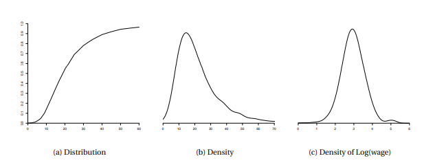
We can estimate $\boldsymbol{\beta}$ from observational data which includes joint measurements on the variables $(y, x)$. For example, supposing we are interested in estimating a wage equation, we would use a dataset with observations on wages (or weekly earnings), education, experience (or age), and demographic characteristics (gender, race, location). One possible dataset is the Current Population Survey (CPS), a survey of U.S. households which includes questions on employment, income, education, and demographic characteristics.

Notationally we wish to distinguish observations from the underlying random variables. The convention in econometrics is to denote observations by appending a subscript $i$ which runs from 1 to $n$, thus the $i^{t h}$ observation is $\left(y_{i}, \boldsymbol{x}{i}\right)$, and $n$ denotes the sample size. The dataset is then $\left{\left(y{i}, \boldsymbol{x}_{i}\right) ; i=1, \ldots, n\right}$. We call this the sample or the observations.

From the viewpoint of empirical analysis a dataset is an array of numbers often organized as a table, where the columns of the table correspond to distinct variables and the rows correspond to distinct observations. For empirical analysis the dataset and observations are fixed in the sense that they are numbers presented to the researcher. For statistical analysis we need to view the dataset as random, or more precisely as a realization of a random process.

In order for the coefficient $\boldsymbol{\beta}$ defined in (3.1) to make sense as defined the expectations over the random variables $(\boldsymbol{x}, y)$ need to be common across the observations. The most elegant approach to ensure this is to assume that the observations are draws from an identical underlying population $F$. This is the standard assumption that the observations are identically distributed:

This assumption does not need to be viewed as literally true, rather it is a useful modeling device so that parameters such as $\boldsymbol{\beta}$ are well defined. This assumption should be interpreted as how we view an observation a priori, before we actually observe it. If I tell you that we have a sample with $n=59$ observations set in no particular order, then it makes sense to view two observations, say 17 and 58 , as draws from the same distribution. We have no reason to expect anything special about either observation.
In econometric theory we refer to the underlying common distribution $F$ as the population. Some authors prefer the label the data-generating-process (DGP). You can think of it as a theoretical concept or an infinitely-large potential population. In contrast we refer to the observations available to us $\left{\left(y_{i}, x_{i}\right): i=1, \ldots, n\right}$ as the sample or dataset. In some contexts the dataset consists of all potential observations, for example administrative tax records may contain every single taxpayer in a political unit. Even in this case we view the observations as if they are random draws from an underlying infinitely-large population as this will allow us to apply the tools of statistical theory.

The linear projection model applies to the random observations $\left(y_{i}, \boldsymbol{x}{l}\right)$. This means that the probability model for the observations is the same as that described in Section $2.18$. We can write the model as $$ y{i}=\boldsymbol{x}{i}^{\prime} \boldsymbol{\beta}+e{i}
$$
where the linear projection coefficient $\boldsymbol{\beta}$ is defined as
$$
\boldsymbol{\beta}=\underset{b \in \mathbb{R}^{k}}{\operatorname{argmin}} S(\boldsymbol{b}),
$$
the minimizer of the expected squared error
$$
S(\boldsymbol{\beta})=\mathbb{E}\left[\left(y_{i}-\boldsymbol{x}{i}^{\prime} \boldsymbol{\beta}\right)^{2}\right] $$ The coefficient has the explicit solution $$ \boldsymbol{\beta}=\left(\mathbb{E}\left[\boldsymbol{x}{i} \boldsymbol{x}{i}^{\prime}\right]\right)^{-1} \mathbb{E}\left[\boldsymbol{x}{i} y_{i}\right]
$$

经济代写|计量经济学作业代写Econometrics代考|Moment Estimators

We want tn estimate the cnefficient $\beta$ defined in (3.5) from the sample of nhservatinns. Nntice that $\boldsymbol{\beta}$ is written as a function of certain population expectations. In this context an appropriate estimator is the same function of the sample moments. Let’s explain this in detail.

To start, suppose that we are interested in the population mean $\mu$ of a random variable $y_{i}$ with dis= tribution function $F$
$$
\mu=\mathbb{E}\left[y_{i}\right]=\int_{-\infty}^{\infty} y d F(y)
$$
The mean $\mu$ is a function of the distribution $F$ as written in (3.6). To estimate $\mu$ given a sample $\left{y_{1}, \ldots, y_{n}\right}$ a natural estimator is the sample mean
$$
\widehat{\jmath}=\bar{y}=\frac{1}{n} \sum_{i=1}^{n} y_{i} .
$$
Notice that we have written this using two pieces of notation. The notation $\bar{y}$ with the bar on top is conventional for a sample mean. The notation $\hat{\mu}$ with the hat ” $\wedge$ ” is conventional in econometrics to

denote an estimator of the parameter $\mu$. In this case $\bar{y}$ is the estimator of $\mu$, so $\widehat{\mu}$ and $\bar{y}$ are the same. The sample mean $\bar{y}$ can be viewed as the natural analog of the population mean (3.6) because $\bar{y}$ equals the expectation (3.6) with respect to the empirical distribution – the discrete distribution which puts weight $1 / n$ on each observation $y_{i}$. There are many other justifications for $\bar{y}$ as an estimator for $\mu$. We will defer these discussions for now. Suffice it to say that it is the conventional estimator in the lack of other information about $\mu$ or the distribution of $y_{i}$.

Now suppose that we are interested in a set of population means of possibly non-linear functions of a random vector $\boldsymbol{y}$, say $\boldsymbol{\mu}=\mathbb{E}\left[\boldsymbol{h}\left(\boldsymbol{y}{i}\right)\right]$. For example, we may be interested in the first two moments of $y{i}$, $\mathbb{E}\left[y_{i}\right]$ and $\mathbb{E}\left[y_{i}^{2}\right]$. In this case the natural estimator is the vector of sample means,
$$
\widehat{\boldsymbol{\mu}}=\frac{1}{n} \sum_{i=1}^{n} \boldsymbol{h}\left(y_{i}\right)
$$
where $\boldsymbol{h}(y)=\left(y, y^{2}\right)$. In this case $\widehat{\mu}{1}=\frac{1}{n} \sum{i=1}^{n} y_{i}$ and $\widehat{\mu}{2}=\frac{1}{n} \sum{i=1}^{n} y_{i}^{2}$. We call $\hat{\boldsymbol{\mu}}$ the moment estimator for $\boldsymbol{\mu}$.

Now suppose that we are interested in a nonlinear function of a set of moments. For example, consider the variance of $y$
$$
\sigma^{2}=\operatorname{var}\left[y_{i}\right]=\mathbb{E}\left[y_{i}^{2}\right]-\left(\mathbb{E}\left[y_{i}\right]\right)^{2} .
$$
In general, many parameters of interest can be written as a function of moments of $\boldsymbol{y}$. Notationally,
$$
\begin{aligned}
&\boldsymbol{\beta}=\boldsymbol{g}(\boldsymbol{\mu}) \
&\boldsymbol{\mu}=\mathbb{E}\left[\boldsymbol{h}\left(\boldsymbol{y}{i}\right)\right] \end{aligned} $$ Here, $\boldsymbol{y}{i}$ are the random variables, $\boldsymbol{h}\left(\boldsymbol{y}{i}\right)$ are functions (transformations) of the random variables, and $\boldsymbol{\mu}$ is the mean (expectation) of these functions. $\boldsymbol{\beta}$ is the parameter of interest, and is the (nonlinear) function $\boldsymbol{g}(\cdot)$ of these means. In this context a natural estimator of $\boldsymbol{\beta}$ is obtained by replacing $\boldsymbol{\mu}$ with $\hat{\boldsymbol{\mu}}$. $$ \begin{aligned} &\widehat{\boldsymbol{\beta}}=\boldsymbol{g}(\widehat{\boldsymbol{\mu}}) \ &\widehat{\boldsymbol{\mu}}=\frac{1}{n} \sum{i=1}^{n} \boldsymbol{h}\left(\boldsymbol{y}{i}\right) . \end{aligned} $$ The estimator $\widehat{\boldsymbol{\beta}}$ is sometimes called a “plug-in” estimator, and sometimes a “substitution” estimator. We typically call $\widehat{\boldsymbol{\beta}}$ a moment, or moment-based, estimator of $\boldsymbol{\beta}$, since it is a natural extension of the moment estimator $\hat{\boldsymbol{\mu}}$. Take the example of the variance $\sigma^{2}=\operatorname{var}\left[y{i}\right]$. Its moment estimator is
$$
\widehat{\sigma}^{2}=\widehat{\mu}{2}-\widehat{\mu}{1}^{2}=\frac{1}{n} \sum_{i=1}^{n} y_{i}^{2}-\left(\frac{1}{n} \sum_{i=1}^{n} y_{i}\right)^{2} .
$$
This is not the only possible estimator for $\sigma^{2}$ (there is also the well-known bias-corrected estimator) but $\widehat{\sigma}^{2}$ is a straightforward and simple choice.

经济代写|计量经济学作业代写Econometrics代考|Least Squares Estimator

The linear projectinn coefficient $\boldsymbol{\beta}$ is defined in (3.3) as the minimizer nf the experted squared errno $S(\overline{\boldsymbol{\beta}})$ defined in (3.4). For given $\overline{\boldsymbol{\beta}}$, the expected squared error is the expectation of the squared error

$\left(y_{i}-\boldsymbol{x}{i}^{\prime} \boldsymbol{\beta}\right)^{2}$. The moment estimator of $S(\boldsymbol{\beta})$ is the sample average: $$ \begin{aligned} \widehat{S}(\boldsymbol{\beta}) &=\frac{1}{n} \sum{i=1}^{n}\left(y_{i}-\boldsymbol{x}{i}^{\prime} \boldsymbol{\beta}\right)^{2} \ &=\frac{1}{n} \operatorname{SSE}(\boldsymbol{\beta}) \end{aligned} $$ where $$ \operatorname{SSE}(\boldsymbol{\beta})=\sum{i=1}^{n}\left(y_{i}-\boldsymbol{x}{i}^{\prime} \boldsymbol{\beta}\right)^{2} $$ is called the sum-of-squared-errors function. Since $\widehat{S}(\boldsymbol{\beta})$ is a sample average we can interpret it as an estimator of the expected squared error $S(\boldsymbol{\beta})$. Examining $\widehat{S}(\boldsymbol{\beta})$ as a function of $\boldsymbol{\beta}$ is informative about how $S(\boldsymbol{\beta})$ varies with $\boldsymbol{\beta}$. Since the projection coefficient minimizes $S(\boldsymbol{\beta})$ an analog estimator minimizes (3.7). We define the estimator $\widehat{\boldsymbol{\beta}}$ as the minimizer of $\widehat{S}(\boldsymbol{\beta})$. Definition 3.1 The least-squares estimator $\widehat{\boldsymbol{\beta}}$ is $$ \begin{gathered} \widehat{\boldsymbol{\beta}}=\underset{\hat{\boldsymbol{\beta} \in \widehat{R}^{l}}}{\operatorname{argmin}} \widehat{S}(\boldsymbol{\beta}) \ \boldsymbol{\beta})=\frac{1}{n} \sum{i=1}^{n}\left(y_{l}-\mathbf{x}{i}^{\prime} \boldsymbol{\beta}\right)^{2} \end{gathered} $$ where $$ \widehat{\boldsymbol{\delta}}(\boldsymbol{\beta})=\frac{1}{n} \sum{l=1}^{n}\left(y_{i}-\boldsymbol{x}{l}^{\prime} \boldsymbol{\beta}\right)^{2} $$ As $\widehat{S}(\boldsymbol{\beta})$ is a scale multiple of $\operatorname{SSE}(\boldsymbol{\beta})$ we may equivalently define $\widehat{\boldsymbol{\beta}}$ as the minimizer of $S S E(\boldsymbol{\beta})$ ). Hence $\widehat{\boldsymbol{\beta}}$ is commonly called the least-squares (LS) estimator of $\boldsymbol{\beta}$. The estimator is also commonly refered to as the ordinary least-squares (OLS) estimator. For the origin of this label see the historical discussion on Adrien-Marie Legendre below. Here, as is common in econometrics, we put a hat ” $\wedge$ ” over the parameter $\boldsymbol{\beta}$ to indicate that $\widehat{\boldsymbol{\beta}}$ is a sample estimate of $\boldsymbol{\beta}$. This is a helpful convention. Just by seeing the symbol $\widehat{\boldsymbol{\beta}}$ we can immediately interpret it as an estimator (because of the hat) of the parameter $\boldsymbol{\beta}$. Sometimes when we want to be explicit about the estimation method, we will write $\widehat{\boldsymbol{\beta}}{\text {ols }}$ to signify that it is the OLLS estimator. It is also common to see the notation $\widehat{\boldsymbol{\beta}}_{n}$, where the subscript ” $n$ ” indicates that the estimator depends on the sample size $n$.

It is important to understand the distinction between population parameters such as $\boldsymbol{\beta}$ and sample estimators such as $\widehat{\boldsymbol{\beta}}$. The population parameter $\boldsymbol{\beta}$ is a non-random feature of the population while the sample estimator $\widehat{\boldsymbol{\beta}}$ is a random feature of a random sample. $\boldsymbol{\beta}$ is fixed, while $\widehat{\boldsymbol{\beta}}$ varies across samples.

经济代写|计量经济学作业代写Econometrics代考|The Algebra of Least Squares

计量经济学代写

经济代写|计量经济学作业代写Econometrics代考|Samples

在部分2.18我们推导出并讨论了是给定X对于一对随机变量(是,X)∈R×Rķ并将其称为线性投影模型。我们现在对估计这个模型的参数感兴趣,特别是投影系数
b=(和[XX′])−1和[X是]
我们可以估计b来自观测数据,其中包括对变量的联合测量(是,X). 例如,假设我们有兴趣估计工资方程,我们将使用一个数据集,其中包含工资(或每周收入)、教育、经验(或年龄)和人口特征(性别、种族、位置)的观察结果。一个可能的数据集是当前人口调查 (CPS),这是一项针对美国家庭的调查,其中包括有关就业、收入、教育和人口特征的问题。

从符号上讲,我们希望将观察结果与潜在的随机变量区分开来。计量经济学的惯例是通过附加下标来表示观察结果一世从 1 到n, 就这样一世吨H观察是(是一世,X一世), 和n表示样本量。那么数据集就是\left{\left(y{i}, \boldsymbol{x}_{i}\right) ; i=1, \ldots, n\right}\left{\left(y{i}, \boldsymbol{x}_{i}\right) ; i=1, \ldots, n\right}. 我们称之为样本或观察。

从经验分析的角度来看,数据集是通常组织为表格的数字数组,其中表格的列对应于不同的变量,而行对应于不同的观察结果。对于经验分析,数据集和观察结果是固定的,因为它们是呈现给研究人员的数字。对于统计分析,我们需要将数据集视为随机的,或者更准确地说是随机过程的实现。

为了系数b在(3.1)中定义的意义在于定义对随机变量的期望(X,是)需要在观察中是共同的。确保这一点的最优雅的方法是假设观察结果来自相同的潜在人群F. 这是观测值同分布的标准假设:

这个假设不需要被视为字面上的真实,而是一个有用的建模设备,因此参数如b定义明确。这个假设应该被解释为我们在实际观察之前如何先验地看待观察。如果我告诉你我们有一个样品n=59没有特定顺序的观察值,那么查看两个观察值(例如 17 和 58 )是有意义的,因为它们来自相同的分布。我们没有理由期待这两种观察有什么特别之处。
在计量经济学理论中,我们指的是潜在的共同分布F作为人口。一些作者更喜欢数据生成过程 (DGP) 的标签。您可以将其视为一个理论概念或无限大的潜在人口。相反,我们指的是我们可用的观察结果\left{\left(y_{i}, x_{i}\right): i=1, \ldots, n\right}\left{\left(y_{i}, x_{i}\right): i=1, \ldots, n\right}作为样本或数据集。在某些情况下,数据集包含所有潜在的观察结果,例如行政税务记录可能包含政治单位中的每个纳税人。即使在这种情况下,我们也将观察结果视为从潜在的无限大群体中随机抽取,因为这将使我们能够应用统计理论的工具。

线性投影模型适用于随机观测(是一世,Xl). 这意味着观察的概率模型与第 1 节中描述的相同2.18. 我们可以将模型写为是一世=X一世′b+和一世
其中线性投影系数b定义为
b=精氨酸b∈Rķ小号(b),
期望平方误差的最小值
小号(b)=和[(是一世−X一世′b)2]系数有显式解b=(和[X一世X一世′])−1和[X一世是一世]

经济代写|计量经济学作业代写Econometrics代考|Moment Estimators

我们要 tn 估计 cnefficientb从 nhservatinns 样本中定义在 (3.5) 中。注意到b被写成某些人口预期的函数。在这种情况下,适当的估计器是样本矩的相同函数。让我们详细解释一下。

首先,假设我们对总体均值感兴趣μ随机变量是一世带分布函数F
μ=和[是一世]=∫−∞∞是dF(是)
均值μ是分布的函数F如(3.6)中所写。估计μ给定一个样本\left{y_{1}, \ldots, y_{n}\right}\left{y_{1}, \ldots, y_{n}\right}自然估计量是样本均值
Ÿ^=是¯=1n∑一世=1n是一世.
请注意,我们使用两种符号来编写它。符号是¯顶部的条形图对于样本均值来说是常规的。符号μ^带着帽子”∧” 在计量经济学中是传统的

表示参数的估计量μ. 在这种情况下是¯是的估计量μ, 所以μ^和是¯是相同的。样本均值是¯可以看作是总体均值 (3.6) 的自然类似物,因为是¯等于关于经验分布的期望(3.6)——赋予权重的离散分布1/n在每次观察是一世. 还有很多其他的理由是¯作为估计器μ. 我们将暂时推迟这些讨论。可以说它是缺乏其他信息的传统估计量μ或分布是一世.

现在假设我们对随机向量的可能非线性函数的一组总体均值感兴趣是, 说μ=和[H(是一世)]. 例如,我们可能对前两个时刻感兴趣是一世, 和[是一世]和和[是一世2]. 在这种情况下,自然估计量是样本均值的向量,
μ^=1n∑一世=1nH(是一世)
在哪里H(是)=(是,是2). 在这种情况下μ^1=1n∑一世=1n是一世和μ^2=1n∑一世=1n是一世2. 我们称之为μ^矩估计器μ.

现在假设我们对一组矩的非线性函数感兴趣。例如,考虑方差是
σ2=曾是⁡[是一世]=和[是一世2]−(和[是一世])2.
通常,许多感兴趣的参数可以写成矩的函数是. 从符号上讲,
b=G(μ) μ=和[H(是一世)]这里,是一世是随机变量,H(是一世)是随机变量的函数(变换),并且μ是这些函数的平均值(期望值)。b是感兴趣的参数,并且是(非线性)函数G(⋅)这些手段中。在这种情况下,自然估计b通过替换获得μ和μ^.b^=G(μ^) μ^=1n∑一世=1nH(是一世).估算器b^有时称为“插件”估计器,有时称为“替代”估计器。我们通常称b^矩或基于矩的估计量b, 因为它是矩估计量的自然延伸μ^. 以方差为例σ2=曾是⁡[是一世]. 它的矩估计量是
σ^2=μ^2−μ^12=1n∑一世=1n是一世2−(1n∑一世=1n是一世)2.
这不是唯一可能的估计量σ2(还有著名的偏差校正估计器)但是σ^2是一个简单明了的选择。

经济代写|计量经济学作业代写Econometrics代考|Least Squares Estimator

线性投影系数b在 (3.3) 中定义为最小化 nf 专家平方 errno小号(b¯)在 (3.4) 中定义。对于给定的b¯,期望平方误差是平方误差的期望

(是一世−X一世′b)2. 矩估计器小号(b)是样本平均值:小号^(b)=1n∑一世=1n(是一世−X一世′b)2 =1n上证所⁡(b)在哪里上证所⁡(b)=∑一世=1n(是一世−X一世′b)2称为误差平方和函数。自从小号^(b)是一个样本平均值,我们可以将其解释为预期平方误差的估计值小号(b). 检查小号^(b)作为一个函数b提供有关如何的信息小号(b)随b. 由于投影系数最小化小号(b)模拟估计器最小化(3.7)。我们定义估计器b^作为最小化器小号^(b). 定义 3.1 最小二乘估计器b^是b^=精氨酸b∈R^l^小号^(b) b)=1n∑一世=1n(是l−X一世′b)2在哪里d^(b)=1n∑l=1n(是一世−Xl′b)2作为小号^(b)是比例倍数上证所⁡(b)我们可以等价地定义b^作为最小化器小号小号和(b))。因此b^通常称为最小二乘 (LS) 估计量b. 估计器通常也称为普通最小二乘 (OLS) 估计器。有关此标签的起源,请参见下面关于 Adrien-Marie Legendre 的历史讨论。在这里,正如计量经济学中常见的那样,我们戴上帽子”∧”过参数b表示b^是一个样本估计b. 这是一个有用的约定。只看符号b^我们可以立即将其解释为参数的估计量(因为帽子)b. 有时当我们想明确估计方法时,我们会写b^奥尔斯 表示它是 OLLS 估计量。看到符号也很常见b^n, 其中下标 ”n” 表示估计量取决于样本量n.

了解人口参数之间的区别很重要,例如b和样本估计器,例如b^. 人口参数b是总体的非随机特征,而样本估计量b^是随机样本的随机特征。b是固定的,而b^因样本而异。

经济代写|计量经济学作业代写Econometrics代考 请认准statistics-lab™

统计代写请认准statistics-lab™. statistics-lab™为您的留学生涯保驾护航。

金融工程代写

金融工程是使用数学技术来解决金融问题。金融工程使用计算机科学、统计学、经济学和应用数学领域的工具和知识来解决当前的金融问题,以及设计新的和创新的金融产品。

非参数统计代写

非参数统计指的是一种统计方法,其中不假设数据来自于由少数参数决定的规定模型;这种模型的例子包括正态分布模型和线性回归模型。

广义线性模型代考

广义线性模型(GLM)归属统计学领域,是一种应用灵活的线性回归模型。该模型允许因变量的偏差分布有除了正态分布之外的其它分布。

术语 广义线性模型(GLM)通常是指给定连续和/或分类预测因素的连续响应变量的常规线性回归模型。它包括多元线性回归,以及方差分析和方差分析(仅含固定效应)。

有限元方法代写

有限元方法(FEM)是一种流行的方法,用于数值解决工程和数学建模中出现的微分方程。典型的问题领域包括结构分析、传热、流体流动、质量运输和电磁势等传统领域。

有限元是一种通用的数值方法,用于解决两个或三个空间变量的偏微分方程(即一些边界值问题)。为了解决一个问题,有限元将一个大系统细分为更小、更简单的部分,称为有限元。这是通过在空间维度上的特定空间离散化来实现的,它是通过构建对象的网格来实现的:用于求解的数值域,它有有限数量的点。边界值问题的有限元方法表述最终导致一个代数方程组。该方法在域上对未知函数进行逼近。[1] 然后将模拟这些有限元的简单方程组合成一个更大的方程系统,以模拟整个问题。然后,有限元通过变化微积分使相关的误差函数最小化来逼近一个解决方案。

tatistics-lab作为专业的留学生服务机构,多年来已为美国、英国、加拿大、澳洲等留学热门地的学生提供专业的学术服务,包括但不限于Essay代写,Assignment代写,Dissertation代写,Report代写,小组作业代写,Proposal代写,Paper代写,Presentation代写,计算机作业代写,论文修改和润色,网课代做,exam代考等等。写作范围涵盖高中,本科,研究生等海外留学全阶段,辐射金融,经济学,会计学,审计学,管理学等全球99%专业科目。写作团队既有专业英语母语作者,也有海外名校硕博留学生,每位写作老师都拥有过硬的语言能力,专业的学科背景和学术写作经验。我们承诺100%原创,100%专业,100%准时,100%满意。

随机分析代写


随机微积分是数学的一个分支,对随机过程进行操作。它允许为随机过程的积分定义一个关于随机过程的一致的积分理论。这个领域是由日本数学家伊藤清在第二次世界大战期间创建并开始的。

时间序列分析代写

随机过程,是依赖于参数的一组随机变量的全体,参数通常是时间。 随机变量是随机现象的数量表现,其时间序列是一组按照时间发生先后顺序进行排列的数据点序列。通常一组时间序列的时间间隔为一恒定值(如1秒,5分钟,12小时,7天,1年),因此时间序列可以作为离散时间数据进行分析处理。研究时间序列数据的意义在于现实中,往往需要研究某个事物其随时间发展变化的规律。这就需要通过研究该事物过去发展的历史记录,以得到其自身发展的规律。

回归分析代写

多元回归分析渐进(Multiple Regression Analysis Asymptotics)属于计量经济学领域,主要是一种数学上的统计分析方法,可以分析复杂情况下各影响因素的数学关系,在自然科学、社会和经济学等多个领域内应用广泛。

MATLAB代写

MATLAB 是一种用于技术计算的高性能语言。它将计算、可视化和编程集成在一个易于使用的环境中,其中问题和解决方案以熟悉的数学符号表示。典型用途包括:数学和计算算法开发建模、仿真和原型制作数据分析、探索和可视化科学和工程图形应用程序开发,包括图形用户界面构建MATLAB 是一个交互式系统,其基本数据元素是一个不需要维度的数组。这使您可以解决许多技术计算问题,尤其是那些具有矩阵和向量公式的问题,而只需用 C 或 Fortran 等标量非交互式语言编写程序所需的时间的一小部分。MATLAB 名称代表矩阵实验室。MATLAB 最初的编写目的是提供对由 LINPACK 和 EISPACK 项目开发的矩阵软件的轻松访问,这两个项目共同代表了矩阵计算软件的最新技术。MATLAB 经过多年的发展,得到了许多用户的投入。在大学环境中,它是数学、工程和科学入门和高级课程的标准教学工具。在工业领域,MATLAB 是高效研究、开发和分析的首选工具。MATLAB 具有一系列称为工具箱的特定于应用程序的解决方案。对于大多数 MATLAB 用户来说非常重要,工具箱允许您学习应用专业技术。工具箱是 MATLAB 函数(M 文件)的综合集合,可扩展 MATLAB 环境以解决特定类别的问题。可用工具箱的领域包括信号处理、控制系统、神经网络、模糊逻辑、小波、仿真等。

R语言代写问卷设计与分析代写
PYTHON代写回归分析与线性模型代写
MATLAB代写方差分析与试验设计代写
STATA代写机器学习/统计学习代写
SPSS代写计量经济学代写
EVIEWS代写时间序列分析代写
EXCEL代写深度学习代写
SQL代写各种数据建模与可视化代写

经济代写|计量经济学作业代写Econometrics代考|Regression Variance

如果你也在 怎样代写计量经济学Econometrics这个学科遇到相关的难题,请随时右上角联系我们的24/7代写客服。

计量经济学,对经济关系的统计和数学分析,通常作为经济预测的基础。这些信息有时被政府用来制定经济政策,也被私人企业用来帮助价格、库存和生产方面的决策。

statistics-lab™ 为您的留学生涯保驾护航 在代写计量经济学Econometrics方面已经树立了自己的口碑, 保证靠谱, 高质且原创的统计Statistics代写服务。我们的专家在代写计量经济学Econometrics代写方面经验极为丰富,各种代写计量经济学Econometrics相关的作业也就用不着说。

我们提供的计量经济学Econometrics及其相关学科的代写,服务范围广, 其中包括但不限于:

  • Statistical Inference 统计推断
  • Statistical Computing 统计计算
  • Advanced Probability Theory 高等概率论
  • Advanced Mathematical Statistics 高等数理统计学
  • (Generalized) Linear Models 广义线性模型
  • Statistical Machine Learning 统计机器学习
  • Longitudinal Data Analysis 纵向数据分析
  • Foundations of Data Science 数据科学基础
Conditional volatility persistence and volatility spillovers in the foreign  exchange market - ScienceDirect
经济代写|计量经济学作业代写Econometrics代考|Regression Variance

经济代写|计量经济学作业代写Econometrics代考|Intercept-Only Model

An important measure of the dispersion about the CEF function is the unconditional variance of the CEF error $e$. We write this as
$$
\sigma^{2}=\operatorname{var}[e]=\mathbb{E}\left[(e-\mathbb{E}[e])^{2}\right]=\mathbb{E}\left[e^{2}\right]
$$
Theorem 2.4.3 implies the following simple but useful result.
Theorem $2.5$ If $E\left[y^{2}\right]<\infty$ then $\sigma^{2}<\infty$.
We can call $\sigma^{2}$ the regression variance or the variance of the regression error. The magnitude of $\sigma^{2}$ measures the amount of variation in $y$ which is not “explained” or accounted for in the conditional mean $\mathbb{E}[y \mid \boldsymbol{x}]$.

The regression variance depends on the regressors $\boldsymbol{x}$. Consider two regressions
$$
\begin{aligned}
&y=\mathbb{E}\left[y \mid x_{1}\right]+e_{1} \
&y=\mathbb{E}\left[y \mid x_{1}, x_{2}\right]+e_{2}
\end{aligned}
$$
We write the two errors distinctly as $e_{1}$ and $e_{2}$ as they are different – changing the conditioning information changes the conditional mean and therefore the regression crror as well.

In our discussion of iterated expectations we have seen that by increasing the conditioning set the conditional expectation reveals greater detail about the distribution of $y$. What is the implication for the regression error?

It turns out that there is a simple relationship. We can think of the conditional mean $\mathbb{E}[y \mid \boldsymbol{x}]$ as the “explained portion” of $y$. The remainder $e=y-\mathbb{E}[y \mid x]$ is the “unexplained portion”. The simple relationship we now derive shows that the variance of this unexplained portion decreases when we condition on more variables. This relationship is monotonic in the sense that increasing the amont of information always decreases the variance of the unexplained portion.
Theorem 2.6 If $E\left[y^{2}\right]<\infty$ then
$$
\operatorname{var}[y] \geq \operatorname{var}\left[y-\mathbb{E}\left[y \mid \boldsymbol{x}{1}\right]\right] \geq \operatorname{var}\left[y-\mathbb{E}\left[y \mid \boldsymbol{x}{1}, \boldsymbol{x}_{2}\right]\right]
$$
Theorem $2.6$ says that the variance of the difference between $y$ and its conditional mean (weakly) decreases whenever an additional variable is added to the conditioning information.
The proof of Theorem $2.6$ is given in Section 2.33.

经济代写|计量经济学作业代写Econometrics代考|Best Predictor

Suppose that given a realized value of $x$ we want to create a prediction or forecast of $y$. We can write any predictor as a function $g(\boldsymbol{x})$ of $\boldsymbol{x}$. The prediction error is the realized difference $y-g(\boldsymbol{x})$. A nonstochastic measure of the magnitude of the prediction error is the expectation of its square
$$
\mathbb{E}\left[(y-g(x))^{2}\right]
$$
We can define the best predictor as the function $g(x)$ which minimizes (2.9). What function is the best predictor? It turns out that the answer is the CEF $m(\boldsymbol{x})$. This holds regardless of the joint distribution of $(y, \boldsymbol{x})$.
To see this, note that the mean squared error of a predictor $g(\boldsymbol{x})$ is
$$
\begin{aligned}
\mathbb{E}\left[(y-g(\boldsymbol{x}))^{2}\right] &=\mathbb{E}\left[(e+m(\boldsymbol{x})-g(\boldsymbol{x}))^{2}\right] \
&=\mathbb{E}\left[e^{2}\right]+2 \mathbb{E}[e(m(\boldsymbol{x})-g(\boldsymbol{x}))]+\mathbb{E}\left[(m(\boldsymbol{x})-g(\boldsymbol{x}))^{2}\right] \
&=\mathbb{E}\left[e^{2}\right] \text { । }\left[(m(\boldsymbol{x}) \quad g(\boldsymbol{x}))^{2}\right] \
& \geq \mathbb{E}\left[e^{2}\right] \
&=\mathbb{E}\left[(y-m(\boldsymbol{x}))^{2}\right]
\end{aligned}
$$

where the first equality makes the substitution $y=m(\boldsymbol{x})+e$ and the third equality uses Theorem $2.4 .4$. The right-hand-side after the third equality is minimized by setting $g(\boldsymbol{x})=m(\boldsymbol{x})$, yielding the inequality in the fourth line. The minimum is finite under the assumption $\mathbb{E}\left[y^{2}\right]<\infty$ as shown by Theorem $2.5$.
We state this formally in the following result.
Theorem 2.7 Conditional Mean as Best Predictor If $E\left[y^{2}\right]<\infty$, then for any predictor $g(x)$,
It may be helpful to consider this result in the context of the intercept-only model
$$
\begin{aligned}
y &=\mu+e \
\mathbb{E}[e] &=0
\end{aligned}
$$
Theorem $2.7$ shows that the best predictor for $y$ (in the class of constants) is the unconditional mean $\mu=\mathbb{E}[y]$, in the sense that the mean minimizes the mean squared prediction error.

经济代写|计量经济学作业代写Econometrics代考|Conditional Variance

While the conditional mean is a good measure of the location of a conditional distribution it does not provide information ahout the spread of the distrihution. A common measure of the dispersion is the conditional variance. We first give the general definition of the conditional variance of a random variable $w$.
Definition 2.1 If $\mathbb{E}\left[w^{2}\right]<\infty$, the conditional variance of $w$ given $\boldsymbol{x}$ is
$$
\operatorname{var}[w \mid \boldsymbol{x}]=\mathbb{E}\left[(w-\mathbb{E}[w \mid \boldsymbol{x}])^{2} \mid \boldsymbol{x}\right]
$$
The conditional variance is distinct from the unconditional variance var $[w]$. The difference is that the conditional variance is a function of the conditioning variables. Notice that the conditional variance is the conditional second moment, centered around the conditional first moment.
Given this definition we define the conditional variance of the regression error.
Definition 2.2 If $\mathbb{E}\left[e^{2}\right]<\infty$, the conditional variance of the regression error $e$ is
$$
\sigma^{2}(\boldsymbol{x})=\operatorname{var}[e \mid \boldsymbol{x}]=\mathbb{E}\left[e^{2} \mid \boldsymbol{x}\right] .
$$

Again, the conditional variance $\sigma^{2}(\boldsymbol{x})$ is distinct from the unconditional variance $\sigma^{2}$. The conditional variance is a function of the regressors, the unconditional variance is not. Generally, $\sigma^{2}(\boldsymbol{x})$ is a non-trivial function of $\boldsymbol{x}$ and can take any form subject to the restriction that it is non-negative. One way to think about $\sigma^{2}(\boldsymbol{x})$ is that it is the conditional mean of $e^{2}$ given $\boldsymbol{x}$. Notice as well that $\sigma^{2}(\boldsymbol{x})=\operatorname{var}[y \mid \boldsymbol{x}]$ so it is equivalently the conditional variance of the dependent variable.

The variance is in a different unit of measurement than the original variable. To convert the variance back to the same unit of measure we define the conditional standard deviation as its square root $\sigma(\boldsymbol{x})=$ $\sqrt{\sigma^{2}(x)}$.

As an example of how the conditional variance depends on observables, compare the conditional log wage densities for men and women displayed in Figure 2.2. The difference between the densities is not purely a location shift but is also a difference in spread. Specifically, we can see that the density for men’s log wages is somewhat more spread out than that for women, while the density for women’s wages is somewhat more peaked. Indeed, the conditional standard deviation for men’s wages is $3.05$ and that for women is $2.81$. So while men have higher average wages they are also somewhat more dispersed.
In general the unconditional variance is related to the conditional variance by the following relationship.
Theorem $2.8$ If $E\left[w^{2}\right]<\infty$ then
$$
\operatorname{var}[w]=\mathbb{E}[\operatorname{var}[w \mid \boldsymbol{x}]]+\operatorname{var}[\mathbb{E}[w \mid \boldsymbol{x}]]
$$
See Theorem $4.14$ of Introduction to Econometrics. Theorem $2.8$ decomposes the unconditional variance into what are sometimes called the “within group variance” and the “across group variance”. For example, if $x$ is education level, then the first term is the expected variance of the conditional means by education level. The second term is the variance after controlling for education.

The regression error has a conditional mean of zero, so its unconditional error variance equals the expected conditional variance, or equivalently can be found by the law of iterated expectations
$$
a^{2}-\mathbb{L}\left[e^{2}\right]-\mathbb{L}\left[\mathbb{L}\left[e^{2} \mid x\right]\right]-\mathbb{L}\left[\sigma^{2}(x)\right]
$$
That is, the unconditional error variance is the average conditional variance.
Given the conditional variance we can define a rescaled error
$$
u=\frac{e}{\sigma(x)}
$$
We can calculate that since $\sigma(x)$ is a function of $\boldsymbol{x}$
$$
\mathbb{E}[u \mid \boldsymbol{x}]=\mathbb{E}\left[\frac{e}{\sigma(\boldsymbol{x})} \mid \boldsymbol{x}\right]=\frac{1}{\sigma(\boldsymbol{x})} \mathbb{E}[e \mid \boldsymbol{x}]=0
$$
and
$$
\operatorname{var}[u \mid \boldsymbol{x}]=\mathbb{E}\left[u^{2} \mid \boldsymbol{x}\right]=\mathbb{E}\left[\frac{e^{2}}{\sigma^{2}(\boldsymbol{x})} \mid \boldsymbol{x}\right]=\frac{1}{\sigma^{2}(\boldsymbol{x})} \mathbb{E}\left[e^{2} \mid \boldsymbol{x}\right]=\frac{\sigma^{2}(\boldsymbol{x})}{\sigma^{2}(\boldsymbol{x})}=1
$$
Thus $u$ has a conditional mean of zero and a conditional variance of 1 .
Notice that (2.10) can be rewritten as
$$
e=\sigma(\boldsymbol{x}) u
$$

Time Variations and Covariations in the Expectation and Volatility of Stock  Market Returns - WHITELAW - 1994 - The Journal of Finance - Wiley Online  Library
经济代写|计量经济学作业代写Econometrics代考|Regression Variance

计量经济学代写

经济代写|计量经济学作业代写Econometrics代考|Intercept-Only Model

CEF 函数离散度的一个重要度量是 CEF 误差的无条件方差和. 我们把它写成
σ2=曾是⁡[和]=和[(和−和[和])2]=和[和2]
定理 2.4.3 暗示了以下简单但有用的结果。
定理2.5如果和[是2]<∞然后σ2<∞.
我们可以打电话σ2回归方差或回归误差的方差。的幅度σ2测量变化量是在条件均值中没有“解释”或说明和[是∣X].

回归方差取决于回归量X. 考虑两个回归
是=和[是∣X1]+和1 是=和[是∣X1,X2]+和2
我们将这两个错误清楚地写为和1和和2因为它们是不同的——改变条件信息会改变条件均值,因此也会改变回归误差。

在我们对迭代期望的讨论中,我们已经看到,通过增加条件集,条件期望揭示了更多关于是. 回归误差的含义是什么?

事实证明,有一个简单的关系。我们可以考虑条件均值和[是∣X]作为“解释部分”是. 剩下的和=是−和[是∣X]是“无法解释的部分”。我们现在推导出的简单关系表明,当我们以更多变量为条件时,这个无法解释的部分的方差会减小。这种关系是单调的,因为增加信息量总是会降低无法解释部分的方差。
定理 2.6 如果和[是2]<∞然后
曾是⁡[是]≥曾是⁡[是−和[是∣X1]]≥曾是⁡[是−和[是∣X1,X2]]
定理2.6表示两者之间的差异的方差是并且每当向条件信息中添加一个附加变量时,其条件均值(微弱)就会减小。
定理的证明2.6在第 2.33 节中给出。

经济代写|计量经济学作业代写Econometrics代考|Best Predictor

假设给定一个已实现的价值X我们想创建一个预测或预测是. 我们可以将任何预测器编写为函数G(X)的X. 预测误差是实现的差异是−G(X). 预测误差大小的非随机度量是其平方的期望
和[(是−G(X))2]
我们可以将最佳预测器定义为函数G(X)最小化(2.9)。什么函数是最好的预测器?原来答案是CEF米(X). 无论联合分布如何,这都成立(是,X).
要看到这一点,请注意预测变量的均方误差G(X)是
।和[(是−G(X))2]=和[(和+米(X)−G(X))2] =和[和2]+2和[和(米(X)−G(X))]+和[(米(X)−G(X))2] =和[和2] । [(米(X)G(X))2] ≥和[和2] =和[(是−米(X))2]

其中第一个等式进行替换是=米(X)+和第三个等式使用定理2.4.4. 通过设置最小化第三个等式后的右侧G(X)=米(X),产生第四行的不等式。在假设下最小值是有限的和[是2]<∞如定理所示2.5.
我们在下面的结果中正式说明了这一点。
定理 2.7 条件均值作为最佳预测器 If和[是2]<∞,那么对于任何预测器G(X),
在仅截取模型的上下文中考虑此结果可能会有所帮助
是=μ+和 和[和]=0
定理2.7表明最好的预测器是(在常量类中)是无条件均值μ=和[是],从某种意义上说,均值使均方预测误差最小化。

经济代写|计量经济学作业代写Econometrics代考|Conditional Variance

虽然条件均值可以很好地衡量条件分布的位置,但它不能提供有关分布分布的信息。分散度的常用度量是条件方差。我们首先给出随机变量的条件方差的一般定义在.
定义 2.1 如果和[在2]<∞, 的条件方差在给定X是
曾是⁡[在∣X]=和[(在−和[在∣X])2∣X]
条件方差不同于无条件方差 var[在]. 不同之处在于条件方差是条件变量的函数。请注意,条件方差是条件二阶矩,以条件一阶矩为中心。
给定这个定义,我们定义回归误差的条件方差。
定义 2.2 如果和[和2]<∞, 回归误差的条件方差和是
σ2(X)=曾是⁡[和∣X]=和[和2∣X].

再次,条件方差σ2(X)不同于无条件方差σ2. 条件方差是回归量的函数,无条件方差不是。一般来说,σ2(X)是一个非平凡的函数X并且可以采取任何形式,但必须限制它是非负的。一种思考方式σ2(X)是它的条件均值和2给定X. 还要注意σ2(X)=曾是⁡[是∣X]所以它等效地是因变量的条件方差。

方差与原始变量的测量单位不同。为了将方差转换回相同的度量单位,我们将条件标准差定义为其平方根σ(X)= σ2(X).

作为条件方差如何依赖于可观察值的示例,比较图 2.2 中显示的男性和女性的条件对数工资密度。密度之间的差异不仅是位置偏移,而且也是传播差异。具体来说,我们可以看到男性的对数工资密度比女性的分布更分散,而女性的工资密度则更峰值。事实上,男性工资的条件标准差是3.05对女性来说是2.81. 因此,虽然男性的平均工资较高,但他们也更加分散。
通常,无条件方差通过以下关系与条件方差相关。
定理2.8如果和[在2]<∞然后
曾是⁡[在]=和[曾是⁡[在∣X]]+曾是⁡[和[在∣X]]
见定理4.14计量经济学导论。定理2.8将无条件方差分解为有时称为“组内方差”和“组间方差”的变量。例如,如果X是教育水平,则第一项是教育水平条件均值的期望方差。第二项是控制教育后的方差。

回归误差的条件均值为零,因此它的无条件误差方差等于期望的条件方差,或者等价地可以通过迭代期望定律找到
一种2−大号[和2]−大号[大号[和2∣X]]−大号[σ2(X)]
也就是说,无条件误差方差是平均条件方差。
给定条件方差,我们可以定义重新调整的误差
在=和σ(X)
我们可以计算出,因为σ(X)是一个函数X
和[在∣X]=和[和σ(X)∣X]=1σ(X)和[和∣X]=0

曾是⁡[在∣X]=和[在2∣X]=和[和2σ2(X)∣X]=1σ2(X)和[和2∣X]=σ2(X)σ2(X)=1
因此在条件均值为零,条件方差为 1 。
注意 (2.10) 可以重写为
和=σ(X)在

经济代写|计量经济学作业代写Econometrics代考 请认准statistics-lab™

统计代写请认准statistics-lab™. statistics-lab™为您的留学生涯保驾护航。

金融工程代写

金融工程是使用数学技术来解决金融问题。金融工程使用计算机科学、统计学、经济学和应用数学领域的工具和知识来解决当前的金融问题,以及设计新的和创新的金融产品。

非参数统计代写

非参数统计指的是一种统计方法,其中不假设数据来自于由少数参数决定的规定模型;这种模型的例子包括正态分布模型和线性回归模型。

广义线性模型代考

广义线性模型(GLM)归属统计学领域,是一种应用灵活的线性回归模型。该模型允许因变量的偏差分布有除了正态分布之外的其它分布。

术语 广义线性模型(GLM)通常是指给定连续和/或分类预测因素的连续响应变量的常规线性回归模型。它包括多元线性回归,以及方差分析和方差分析(仅含固定效应)。

有限元方法代写

有限元方法(FEM)是一种流行的方法,用于数值解决工程和数学建模中出现的微分方程。典型的问题领域包括结构分析、传热、流体流动、质量运输和电磁势等传统领域。

有限元是一种通用的数值方法,用于解决两个或三个空间变量的偏微分方程(即一些边界值问题)。为了解决一个问题,有限元将一个大系统细分为更小、更简单的部分,称为有限元。这是通过在空间维度上的特定空间离散化来实现的,它是通过构建对象的网格来实现的:用于求解的数值域,它有有限数量的点。边界值问题的有限元方法表述最终导致一个代数方程组。该方法在域上对未知函数进行逼近。[1] 然后将模拟这些有限元的简单方程组合成一个更大的方程系统,以模拟整个问题。然后,有限元通过变化微积分使相关的误差函数最小化来逼近一个解决方案。

tatistics-lab作为专业的留学生服务机构,多年来已为美国、英国、加拿大、澳洲等留学热门地的学生提供专业的学术服务,包括但不限于Essay代写,Assignment代写,Dissertation代写,Report代写,小组作业代写,Proposal代写,Paper代写,Presentation代写,计算机作业代写,论文修改和润色,网课代做,exam代考等等。写作范围涵盖高中,本科,研究生等海外留学全阶段,辐射金融,经济学,会计学,审计学,管理学等全球99%专业科目。写作团队既有专业英语母语作者,也有海外名校硕博留学生,每位写作老师都拥有过硬的语言能力,专业的学科背景和学术写作经验。我们承诺100%原创,100%专业,100%准时,100%满意。

随机分析代写


随机微积分是数学的一个分支,对随机过程进行操作。它允许为随机过程的积分定义一个关于随机过程的一致的积分理论。这个领域是由日本数学家伊藤清在第二次世界大战期间创建并开始的。

时间序列分析代写

随机过程,是依赖于参数的一组随机变量的全体,参数通常是时间。 随机变量是随机现象的数量表现,其时间序列是一组按照时间发生先后顺序进行排列的数据点序列。通常一组时间序列的时间间隔为一恒定值(如1秒,5分钟,12小时,7天,1年),因此时间序列可以作为离散时间数据进行分析处理。研究时间序列数据的意义在于现实中,往往需要研究某个事物其随时间发展变化的规律。这就需要通过研究该事物过去发展的历史记录,以得到其自身发展的规律。

回归分析代写

多元回归分析渐进(Multiple Regression Analysis Asymptotics)属于计量经济学领域,主要是一种数学上的统计分析方法,可以分析复杂情况下各影响因素的数学关系,在自然科学、社会和经济学等多个领域内应用广泛。

MATLAB代写

MATLAB 是一种用于技术计算的高性能语言。它将计算、可视化和编程集成在一个易于使用的环境中,其中问题和解决方案以熟悉的数学符号表示。典型用途包括:数学和计算算法开发建模、仿真和原型制作数据分析、探索和可视化科学和工程图形应用程序开发,包括图形用户界面构建MATLAB 是一个交互式系统,其基本数据元素是一个不需要维度的数组。这使您可以解决许多技术计算问题,尤其是那些具有矩阵和向量公式的问题,而只需用 C 或 Fortran 等标量非交互式语言编写程序所需的时间的一小部分。MATLAB 名称代表矩阵实验室。MATLAB 最初的编写目的是提供对由 LINPACK 和 EISPACK 项目开发的矩阵软件的轻松访问,这两个项目共同代表了矩阵计算软件的最新技术。MATLAB 经过多年的发展,得到了许多用户的投入。在大学环境中,它是数学、工程和科学入门和高级课程的标准教学工具。在工业领域,MATLAB 是高效研究、开发和分析的首选工具。MATLAB 具有一系列称为工具箱的特定于应用程序的解决方案。对于大多数 MATLAB 用户来说非常重要,工具箱允许您学习应用专业技术。工具箱是 MATLAB 函数(M 文件)的综合集合,可扩展 MATLAB 环境以解决特定类别的问题。可用工具箱的领域包括信号处理、控制系统、神经网络、模糊逻辑、小波、仿真等。

R语言代写问卷设计与分析代写
PYTHON代写回归分析与线性模型代写
MATLAB代写方差分析与试验设计代写
STATA代写机器学习/统计学习代写
SPSS代写计量经济学代写
EVIEWS代写时间序列分析代写
EXCEL代写深度学习代写
SQL代写各种数据建模与可视化代写

经济代写|计量经济学作业代写Econometrics代考|Conditional Expectation Function

如果你也在 怎样代写计量经济学Econometrics这个学科遇到相关的难题,请随时右上角联系我们的24/7代写客服。

计量经济学,对经济关系的统计和数学分析,通常作为经济预测的基础。这些信息有时被政府用来制定经济政策,也被私人企业用来帮助价格、库存和生产方面的决策。

statistics-lab™ 为您的留学生涯保驾护航 在代写计量经济学Econometrics方面已经树立了自己的口碑, 保证靠谱, 高质且原创的统计Statistics代写服务。我们的专家在代写计量经济学Econometrics代写方面经验极为丰富,各种代写计量经济学Econometrics相关的作业也就用不着说。

我们提供的计量经济学Econometrics及其相关学科的代写,服务范围广, 其中包括但不限于:

  • Statistical Inference 统计推断
  • Statistical Computing 统计计算
  • Advanced Probability Theory 高等概率论
  • Advanced Mathematical Statistics 高等数理统计学
  • (Generalized) Linear Models 广义线性模型
  • Statistical Machine Learning 统计机器学习
  • Longitudinal Data Analysis 纵向数据分析
  • Foundations of Data Science 数据科学基础
经济代写|计量经济学作业代写Econometrics代考|Conditional Expectation Function

经济代写|计量经济学作业代写Econometrics代考|Conditional Expectation Function

An important determinant of wage levels is education. In many empirical studies economists measure educational attainment by the number of years ${ }^{8}$ of schooling. We will write this variable as education.

The conditional mean of log wages given gender, race, and education is a single number for each

category. For example
$$
\mathbb{E}[\log (\text { wage }) \mid \text { gender }=\text { man, } \text { race }=\text { white, education }=12]=2.84 .
$$
We display in Figure $2.3$ the conditional means of $\log ($ wage $)$ for white men and white women as a function of education. The plot is quite revealing. We see that the conditional mean is increasing in years of education, but at a different rate for schooling levels above and below nine years. Another striking feature of Figure $2.3$ is that the gap between men and women is roughly constant for all education levels. As the variables are measured in logs this implies a constant average percentage gap between men and women regardless of educational attainment.

In many cases it is convenient to simplify the notation by writing variables using single characters, typically $y, x$ and/or $z$. It is conventional in econometrics to denote the dependent variable (e.g. $\log ($ wage) ) by the letter $y$, a conditioning variable (such as gender) by the letter $x$, and multiple conditioning variables (such as race, education and gender) by the subscripted letters $x_{1}, x_{2}, \ldots, x_{k}$.
Conditional expectations can be written with the generic notation
$$
\mathbb{E}\left[y \mid x_{1}, x_{2}, \ldots, x_{k}\right]=m\left(x_{1}, x_{2}, \ldots, x_{k}\right)
$$
We call this the conditional expectation function (CEF). The CEF is a function of $\left(x_{1}, x_{2}, \ldots, x_{k}\right)$ as it varies with the variables. For example, the conditional expectation of $y=\log ($ wage $)$ given $\left(x_{1}, x_{2}\right)=($ gender, race) is given by the six entries of Table??. The CEF is a function of (gender, race) as it varies across the entries.
For greater compactness, we will typically write the conditioning variables as a vector in $\mathbb{R}^{k}$ :
$$
\boldsymbol{x}=\left(\begin{array}{c}
x_{1} \
x_{2} \
\vdots \
x_{k}
\end{array}\right)
$$

Here we follow the convention of using lower case bold italics $\boldsymbol{x}$ to denote a vector. Given this notation, the CEF can be compactly written as
$$
\mathbb{E}[y \mid \boldsymbol{x}]=m(\boldsymbol{x}) \text {. }
$$
The CEFE $[y \mid \boldsymbol{x}]$ is a random variable as it is a function of the random variable $\boldsymbol{x}$. It is also sometimes useful to view the CEF as a function of $\boldsymbol{x}$. In this case we can write $m(\boldsymbol{u})=\mathbb{E}[y \mid \boldsymbol{x}=\boldsymbol{u}]$, which is a function of the argument $\boldsymbol{u}$. The expression $\mathbb{E}|y| \boldsymbol{x}=\boldsymbol{u} \mid$ is the conditional expectation of $y$, given that we know that the random variable $\boldsymbol{x}$ equals the specific value $\boldsymbol{u}$. However, sometimes in econometrics we take a notational shortcut and use $\mathbb{E}[y \mid x]$ to refer to this function. Hopefully, the use of $E[y \mid x]$ should be apparent from the context.

经济代写|计量经济学作业代写Econometrics代考|Continuous Variables

In the previous sections, we implicitly assumed that the conditioning variables are discrete. However, many conditioning variables are continuous. In this section, we take up this case and assume that the variables $(y, \boldsymbol{x})$ are continuously distributed with a joint density function $f(y, \boldsymbol{x})$.

As an example, take $y=\log ($ wage $)$ and $x=$ experience, the number of years of potential labor market experience ${ }^{9}$. The contours of their joint density are plotted on the left side of Figure $2.4$ for the population of white men with 12 years of education.

Given the joint density $f(y, \boldsymbol{x})$ the variable $\boldsymbol{x}$ has the marginal density
$$
f_{x}(\boldsymbol{x})=\int_{-\infty}^{\infty} f\left(y_{1} \boldsymbol{x}\right) d y
$$
For any $\boldsymbol{x}$ such that $f_{x}(\boldsymbol{x})>0$ the conditional density of $y$ given $\boldsymbol{x}$ is defined as
$$
f_{y \backslash x}(y \mid x)=\frac{f(y, \boldsymbol{x})}{f_{x}(\boldsymbol{x})} .
$$

The conditional density is a (renormalized) slice of the joint density $f(y, x)$ holding $\boldsymbol{x}$ fixed. The slice is renormalized (divided by $f_{x}(\boldsymbol{x})$ so that it integrates to one and is thus a density.) We can visualize this by slicing the joint density function at a specific value of $\boldsymbol{x}$ parallel with the $y$-axis. For example, take the density contours on the left side of Figure $2.4$ and slice through the contour plot at a specific value of experience, and then renormalize the slice so that it is a proper density. This gives us the conditional density of $\log ($ wage $)$ for white men with 12 years of education and this level of experience. We do this for four levels of experience $(5,10,25$, and 40 years), and plot these densities on the right side of Figure 2.4. We can see that the distribution of wages shifts to the right and becomes more diffuse as experience increases from 5 to 10 years, and from 10 to 25 years, but there is little change from 25 to 40 years experience.
The CEF of $y$ given $x$ is the mean of the conditional density (2.4)
$$
m(\boldsymbol{x})=\mathbb{E}[y \mid \boldsymbol{x}]=\int_{-\infty}^{\infty} y f_{y \mid x}(y \mid x) d y .
$$
Intuitively, $m(\boldsymbol{x})$ is the mean of $y$ for the idealized subpopulation where the conditioning variables are fixed at $\boldsymbol{x}$. This is idealized since $\boldsymbol{x}$ is continuously distributed so this subpopulation is infinitely small.
This definition (2.5) is appropriate when the conditional density (2.4) is well defined. However, the conditional mean $m(\boldsymbol{x})$ exists quite generally. In Theorem $2.13$ in Section $2.31$ we show that $m(\boldsymbol{x})$ exists solong as $\mathbb{E}|y|<\infty$.

In Figure $2.4$ the CEF of log(wage) given experience is plotted as the solid line. We can see that the CEF is a smooth but nonlinear function. The CEF is initially increasing in experience, flattens out around experience $=30$, and then decreases for high levels of experience.

经济代写|计量经济学作业代写Econometrics代考|Law of Iterated Expectations

An extremely useful tool from probability theory is the law of iterated expectations. An important special case is the known as the Simple Law.
Theorem 2.1 Simple Law of Iterated Expectations If $E|y|<\infty$ then for any random vector $\boldsymbol{x}$,
$$
\mathbb{E}[\mathbb{E}[y \mid x]]=\mathbb{E}[y]
$$
The simple law states that the expectation of the conditional expectation is the unconditional expectation. In other words the average of the conditional averages is the unconditional average. When $\boldsymbol{x}$ is discrete
$$
\mathbb{E}[\mathbb{E}[y \mid x]]=\sum_{j=1}^{\infty} \mathbb{E}\left[y \mid x=x_{j}\right] \mathbb{P}\left[x=x_{j}\right]
$$
and when $\boldsymbol{x}$ is continuous
$$
\mathbb{E}[\mathbb{E}[y \mid \boldsymbol{x}]]=\int_{\mathrm{x}^{k}} \mathbb{E}[y \mid \boldsymbol{x}] f_{x}(\boldsymbol{x}) d \boldsymbol{x} \text {. }
$$
Going back to our investigation of average log wages for men and women, the simple law states that
$$
\begin{aligned}
&\mathbb{E}[\log (\text { wage }) \mid \text { gender }=\text { man }] \mathbb{P}[\text { gender }=\text { man }] \
&+\mathbb{E}[\log (\text { wage }) \mid \text { gender }=\text { woman }] \mathbb{P}[\text { gender }=\text { woman }] \
&=\mathbb{E}[\log (\text { wage })]
\end{aligned}
$$

Or numerically,
$$
3.05 \times 0.57+2.81 \times 0.43=2.95 .
$$
The general law of iterated expectations allows two sets of conditioning variables.

经济代写|计量经济学作业代写Econometrics代考|Conditional Expectation Function

计量经济学代写

经济代写|计量经济学作业代写Econometrics代考|Conditional Expectation Function

工资水平的一个重要决定因素是教育。在许多实证研究中,经济学家通过年数来衡量教育程度8上学的。我们将把这个变量写成教育。

给定性别、种族和教育的对数工资的条件平均值是每个

类别。例如
和[日志⁡( 工资 )∣ 性别 = 男人,  种族 = 白色, 教育 =12]=2.84.
如图所示2.3的条件手段日志⁡(工资)对白人男性和白人女性来说是教育的一项功能。剧情相当有内涵。我们看到条件均值随着受教育年限的增加而增加,但在九年以上和以下的受教育水平上的增加速度不同。图的另一个显着特点2.3是男女之间的差距在所有教育水平上大致保持不变。由于变量是用对数来衡量的,这意味着无论受教育程度如何,男性和女性之间的平均百分比差距都是恒定的。

在许多情况下,通过使用单个字符编写变量来简化符号很方便,通常是,X和/或和. 在计量经济学中,通常用因变量来表示(例如日志⁡(工资))按信是,由字母组成的条件变量(如性别)X,以及多个条件变量(例如种族、教育和性别),由下标字母表示X1,X2,…,Xķ.
条件期望可以用通用符号来写
和[是∣X1,X2,…,Xķ]=米(X1,X2,…,Xķ)
我们称之为条件期望函数(CEF)。CEF 是一个函数(X1,X2,…,Xķ)因为它随变量而变化。例如,条件期望是=日志⁡(工资)给定(X1,X2)=(性别,种族)由表??的六个条目给出。CEF 是(性别、种族)的函数,因为它因条目而异。
为了更紧凑,我们通常将条件变量写成一个向量Rķ :
X=(X1 X2 ⋮ Xķ)

这里我们遵循使用小写粗斜体的惯例X来表示一个向量。给定这个符号,CEF 可以紧凑地写为
和[是∣X]=米(X). 
CEFE[是∣X]是随机变量,因为它是随机变量的函数X. 有时将 CEF 视为X. 在这种情况下,我们可以写米(在)=和[是∣X=在],它是参数的函数在. 表达方式和|是|X=在∣是条件期望是,假设我们知道随机变量X等于特定值在. 然而,有时在计量经济学中,我们采用符号捷径并使用和[是∣X]参考这个功能。希望使用和[是∣X]从上下文中应该是显而易见的。

经济代写|计量经济学作业代写Econometrics代考|Continuous Variables

在前面的部分中,我们隐含地假设条件变量是离散的。然而,许多条件变量是连续的。在本节中,我们采用这种情况并假设变量(是,X)以联合密度函数连续分布F(是,X).

举个例子,取是=日志⁡(工资)和X=经验,潜在劳动力市场经验的年数9. 它们的联合密度等值线绘制在图的左侧2.4适用于受过 12 年教育的白人男性。

给定联合密度F(是,X)变量X有边际密度
FX(X)=∫−∞∞F(是1X)d是
对于任何X这样FX(X)>0的条件密度是给定X定义为
F是∖X(是∣X)=F(是,X)FX(X).

条件密度是关节密度的(重新归一化的)切片F(是,X)保持X固定的。切片被重新归一化(除以FX(X)因此它集成为一个,因此是一个密度。)我们可以通过将联合密度函数切片为特定值来可视化这一点X与是-轴。例如,取图左侧的密度等高线2.4并以特定的经验值对等高线图进行切片,然后对切片进行重新归一化,使其具有适当的密度。这给了我们条件密度日志⁡(工资)适用于受过 12 年教育并具有此经验水平的白人男性。我们这样做是为了四个级别的经验(5,10,25和 40 年),并在图 2.4 的右侧绘制这些密度。我们可以看到,随着经验从 5 年增加到 10 年,从 10 年增加到 25 年,工资的分布向右移动并且变得更加分散,但是从 25 年到 40 年的经验几乎没有变化。
的 CEF是给定X是条件密度的平均值 (2.4)
米(X)=和[是∣X]=∫−∞∞是F是∣X(是∣X)d是.
直觉上,米(X)是平均值是对于条件变量固定为的理想化亚群X. 这是理想化的,因为X是连续分布的,所以这个亚群是无限小的。
当条件密度(2.4)定义明确时,这个定义(2.5)是合适的。然而,条件均值米(X)相当普遍地存在。定理2.13在部分2.31我们证明了米(X)只要存在和|是|<∞.

如图2.4给定经验的 log(wage) 的 CEF 绘制为实线。我们可以看到 CEF 是一个平滑但非线性的函数。CEF 最初在经验上增加,在经验周围变平=30,然后随着经验水平的提高而降低。

经济代写|计量经济学作业代写Econometrics代考|Law of Iterated Expectations

概率论中一个非常有用的工具是迭代期望定律。一个重要的特殊情况是被称为简单定律的。
定理 2.1 迭代期望的简单定律 If和|是|<∞然后对于任何随机向量X,
和[和[是∣X]]=和[是]
简单定律指出,有条件的期望是无条件的期望。换句话说,条件平均值的平均值是无条件平均值。什么时候X是离散的
和[和[是∣X]]=∑j=1∞和[是∣X=Xj]磷[X=Xj]
什么时候X是连续的
和[和[是∣X]]=∫Xķ和[是∣X]FX(X)dX. 
回到我们对男性和女性平均原木工资的调查,简单的法律规定:
和[日志⁡( 工资 )∣ 性别 = 男人 ]磷[ 性别 = 男人 ] +和[日志⁡( 工资 )∣ 性别 = 女士 ]磷[ 性别 = 女士 ] =和[日志⁡( 工资 )]

或者在数字上,
3.05×0.57+2.81×0.43=2.95.
迭代期望的一般规律允许两组条件变量。

经济代写|计量经济学作业代写Econometrics代考 请认准statistics-lab™

统计代写请认准statistics-lab™. statistics-lab™为您的留学生涯保驾护航。

金融工程代写

金融工程是使用数学技术来解决金融问题。金融工程使用计算机科学、统计学、经济学和应用数学领域的工具和知识来解决当前的金融问题,以及设计新的和创新的金融产品。

非参数统计代写

非参数统计指的是一种统计方法,其中不假设数据来自于由少数参数决定的规定模型;这种模型的例子包括正态分布模型和线性回归模型。

广义线性模型代考

广义线性模型(GLM)归属统计学领域,是一种应用灵活的线性回归模型。该模型允许因变量的偏差分布有除了正态分布之外的其它分布。

术语 广义线性模型(GLM)通常是指给定连续和/或分类预测因素的连续响应变量的常规线性回归模型。它包括多元线性回归,以及方差分析和方差分析(仅含固定效应)。

有限元方法代写

有限元方法(FEM)是一种流行的方法,用于数值解决工程和数学建模中出现的微分方程。典型的问题领域包括结构分析、传热、流体流动、质量运输和电磁势等传统领域。

有限元是一种通用的数值方法,用于解决两个或三个空间变量的偏微分方程(即一些边界值问题)。为了解决一个问题,有限元将一个大系统细分为更小、更简单的部分,称为有限元。这是通过在空间维度上的特定空间离散化来实现的,它是通过构建对象的网格来实现的:用于求解的数值域,它有有限数量的点。边界值问题的有限元方法表述最终导致一个代数方程组。该方法在域上对未知函数进行逼近。[1] 然后将模拟这些有限元的简单方程组合成一个更大的方程系统,以模拟整个问题。然后,有限元通过变化微积分使相关的误差函数最小化来逼近一个解决方案。

tatistics-lab作为专业的留学生服务机构,多年来已为美国、英国、加拿大、澳洲等留学热门地的学生提供专业的学术服务,包括但不限于Essay代写,Assignment代写,Dissertation代写,Report代写,小组作业代写,Proposal代写,Paper代写,Presentation代写,计算机作业代写,论文修改和润色,网课代做,exam代考等等。写作范围涵盖高中,本科,研究生等海外留学全阶段,辐射金融,经济学,会计学,审计学,管理学等全球99%专业科目。写作团队既有专业英语母语作者,也有海外名校硕博留学生,每位写作老师都拥有过硬的语言能力,专业的学科背景和学术写作经验。我们承诺100%原创,100%专业,100%准时,100%满意。

随机分析代写


随机微积分是数学的一个分支,对随机过程进行操作。它允许为随机过程的积分定义一个关于随机过程的一致的积分理论。这个领域是由日本数学家伊藤清在第二次世界大战期间创建并开始的。

时间序列分析代写

随机过程,是依赖于参数的一组随机变量的全体,参数通常是时间。 随机变量是随机现象的数量表现,其时间序列是一组按照时间发生先后顺序进行排列的数据点序列。通常一组时间序列的时间间隔为一恒定值(如1秒,5分钟,12小时,7天,1年),因此时间序列可以作为离散时间数据进行分析处理。研究时间序列数据的意义在于现实中,往往需要研究某个事物其随时间发展变化的规律。这就需要通过研究该事物过去发展的历史记录,以得到其自身发展的规律。

回归分析代写

多元回归分析渐进(Multiple Regression Analysis Asymptotics)属于计量经济学领域,主要是一种数学上的统计分析方法,可以分析复杂情况下各影响因素的数学关系,在自然科学、社会和经济学等多个领域内应用广泛。

MATLAB代写

MATLAB 是一种用于技术计算的高性能语言。它将计算、可视化和编程集成在一个易于使用的环境中,其中问题和解决方案以熟悉的数学符号表示。典型用途包括:数学和计算算法开发建模、仿真和原型制作数据分析、探索和可视化科学和工程图形应用程序开发,包括图形用户界面构建MATLAB 是一个交互式系统,其基本数据元素是一个不需要维度的数组。这使您可以解决许多技术计算问题,尤其是那些具有矩阵和向量公式的问题,而只需用 C 或 Fortran 等标量非交互式语言编写程序所需的时间的一小部分。MATLAB 名称代表矩阵实验室。MATLAB 最初的编写目的是提供对由 LINPACK 和 EISPACK 项目开发的矩阵软件的轻松访问,这两个项目共同代表了矩阵计算软件的最新技术。MATLAB 经过多年的发展,得到了许多用户的投入。在大学环境中,它是数学、工程和科学入门和高级课程的标准教学工具。在工业领域,MATLAB 是高效研究、开发和分析的首选工具。MATLAB 具有一系列称为工具箱的特定于应用程序的解决方案。对于大多数 MATLAB 用户来说非常重要,工具箱允许您学习应用专业技术。工具箱是 MATLAB 函数(M 文件)的综合集合,可扩展 MATLAB 环境以解决特定类别的问题。可用工具箱的领域包括信号处理、控制系统、神经网络、模糊逻辑、小波、仿真等。

R语言代写问卷设计与分析代写
PYTHON代写回归分析与线性模型代写
MATLAB代写方差分析与试验设计代写
STATA代写机器学习/统计学习代写
SPSS代写计量经济学代写
EVIEWS代写时间序列分析代写
EXCEL代写深度学习代写
SQL代写各种数据建模与可视化代写

经济代写|计量经济学作业代写Econometrics代考|Conditional Expectation and Projection

如果你也在 怎样代写计量经济学Econometrics这个学科遇到相关的难题,请随时右上角联系我们的24/7代写客服。

计量经济学,对经济关系的统计和数学分析,通常作为经济预测的基础。这些信息有时被政府用来制定经济政策,也被私人企业用来帮助价格、库存和生产方面的决策。

statistics-lab™ 为您的留学生涯保驾护航 在代写计量经济学Econometrics方面已经树立了自己的口碑, 保证靠谱, 高质且原创的统计Statistics代写服务。我们的专家在代写计量经济学Econometrics代写方面经验极为丰富,各种代写计量经济学Econometrics相关的作业也就用不着说。

我们提供的计量经济学Econometrics及其相关学科的代写,服务范围广, 其中包括但不限于:

  • Statistical Inference 统计推断
  • Statistical Computing 统计计算
  • Advanced Probability Theory 高等概率论
  • Advanced Mathematical Statistics 高等数理统计学
  • (Generalized) Linear Models 广义线性模型
  • Statistical Machine Learning 统计机器学习
  • Longitudinal Data Analysis 纵向数据分析
  • Foundations of Data Science 数据科学基础
经济代写|计量经济学作业代写Econometrics代考|Conditional Expectation and Projection

经济代写|计量经济学作业代写Econometrics代考|The Distribution of Wages

Suppose that we are interested in wage rates in the United States. Since wage rates vary across workers, we cannot describe wage rates by a single number. Instead, we can describe wages using a probability distribution. Formally, we view the wage of an individual worker as a random variable wage with the probability distribution
$$
F(u)=\mathbb{P}[w a g e \leq u]
$$
When we say that a person’s wage is random we mean that we do not know their wage before it is measured, and we treat observed wage rates as realizations from the distribution $F$. Treating unobserved wages as random variables and observed wages as realizations is a powerful mathematical abstraction which allows us to use the tools of mathematical probability.

A useful thought experiment is to imagine dialing a telephone number selected at random, and then asking the person who responds tn tell ws their wage rate. (Assıme for simplicity that all workers have. equal access to telephones, and that the person who answers your call will respond honestly.) In this thought experiment, the wage of the person you have called is a single draw from the distribution $F$ of wages in the population. By making many such phone calls we can learn the distribution $F$ of the entire population.
When a distribution function $F$ is differentiable we define the probability density function
$$
f(u)=\frac{d}{d u} F(u) .
$$
The density contains the same information as the distribution function, but the density is typically easier to visually interpret.

In Figure $2.1$ we display estimates ${ }^{1}$ of the probability distribution function (panel (a)) and density function (panel (b)) of U.S. wage rates in 2009 . We see that the density is peaked around $\$ 15$, and most of the probability mass appears to lie between $\$ 10$ and $\$ 40$. These are ranges for typical wage rates in the U.S. population.

Important measures of central tendency are the median and the mean. The median $m$ of a continuous ${ }^{2}$ distribution $F$ is the unique solution to
$$
F(m)=\frac{1}{2}
$$
The median U.S. wage is $\$ 19.23$. The median is a robust ${ }^{3}$ measure of central tendency, but it is tricky to use for many calculations as it is not a linear operator.
The expectation or mean of a random variable $y$ with discrete support is
$$
\mu=\mathbb{E}[y]=\sum_{j=1}^{\infty} \tau_{j} \mathbb{P}\left[y=\tau_{j}\right]
$$
For a continuous random variable with density $f(y)$ the expectation is
$$
\mu=\mathbb{E}[y]=\int_{-\infty}^{\infty} y f(y) d y .
$$
Here we have used the common and convenient convention of using the single character $y$ to denote a random variable, rather than the more cumbersome label wage. We sometimes use the notation Ey instead of $E[y]$ when the variable whose expectation is being taken is clear from the context. There is no distinction in meaning. An alternative notation which includes both discrete and continuous random variables as special cases is
$$
\mu=\mathbb{E}[y]=\int_{-\infty}^{\infty} y d F(y)
$$

经济代写|计量经济学作业代写Econometrics代考|Conditional Expectation

We saw in Figure ?? the density of log wages. Is this distribution the same for all workers, or does the wage distribution vary across subpopulations? To answer this question, we can compare wage distributions for different groups – for example, men and women. The plot on the left in Figure $2.2$ displays the densities of log wages for U.S. men and women. We can see that the two wage densities take similar shapes but the density for men is somewhat shifted to the right.

The values $3.05$ and $2.81$ are the mean log wages in the subpopulations of men and women workers. They are called the conditional means (or conditional expectations) of log wages given gender. We can write their specific values as
$$
\begin{gathered}
\mathbb{E}[\log (\text { wage }) \mid \text { gender }=\text { man }]=3.05 \
\mathbb{E}[\log (\text { wage }) \mid \text { gender }=\text { woman }]=2.81 .
\end{gathered}
$$
We call these means conditional as they are conditioning on a fixed value of the variable gender. While you might not think of a person’s gender as a random variable, it is random from the viewpoint of econometric analysis. If you randomly select an individual, the gender of the individual is unknown and thus random. (In the population of U.S. workers, the probability that a worker is a woman happens to be 43\%.) In observational data, it is most appropriate to view all measurements as random variables, and the means of subpopulatlons are then conditlonal means.

As the two densities in Figure $2.2$ appear similar, a hasty inference might be that there is not a meaningful difference between the wage distributions of men and women. Before jumping to this conclusion let us examine the differences in the distributions more carefully. As we mentioned above, the primary difference between the two densities appears to be their means. This difference equals
$$
\begin{aligned}
\mathbb{E}[\log (\text { wage }) \mid \text { gender }=\text { man }]-\mathbb{E}[\log (\text { wage }) \mid \text { gender }=\text { woman }] &=3.05-2.81 \
&=0.24 .
\end{aligned}
$$
A difference in expected log wages of $0.24$ is often interpreted as an average $24 \%$ difference between the wages of men and women, which is quite substantial. (For a more complete explanation see Section 2.4.)
Consider further splitting the men and women subpopulations by race, dividing the population into whites, blacks, and other races. We display the log wage density functions of four of these groups on the right in Figure 2.2. Again we see that the primary difference between the four density functions is their central tendency.

Focusing on the means of these distributions, Table $2.1$ reports the mean log wage for each of the six sub-populations.
Table 2.1: Mean Log Wages by Gender and Race
\begin{tabular}{lcc}
\hline \hline & men & women \
\cline { 2 – 3 } white & $3.07$ & $2.82$ \
black & $2.86$ & $2.73$ \
other & $3.03$ & $2.86$ \
\hline
\end{tabular}
The entries in Table $2.1$ are the conditional means of $\log ($ wage $)$ given gender and race. For example
$$
\mathbb{E}[\log (\text { wage }) \mid \text { gender }=\text { man, race }=\text { white }]=3.07
$$
and
$$
\mathbb{E}[\log (\text { wage }) \mid \text { gender }=\text { woman }, \text { race }=\text { black }]=2.73
$$

经济代写|计量经济学作业代写Econometrics代考|Log Differences

A useful approximation for the natural logarithm for small $x$ is
$$
\log (1+x) \approx x
$$
This can be derived from the infinite series expansion of $\log (1+x)$ :
$$
\begin{aligned}
\log (1+x) &=x-\frac{x^{2}}{2}+\frac{x^{3}}{3}-\frac{x^{4}}{4}+\cdots \
&=x+O\left(x^{2}\right)
\end{aligned}
$$
The symbol $O\left(x^{2}\right)$ means that the remainder is bounded by $A x^{2}$ as $x \rightarrow 0$ for some $A<\infty$. Numerically, the approximation $\log (1+x) \simeq x$ is within $0.001$ for $|x| \leq 0.1$. The approximation error increases with $|x|$.
If $y^{}$ is $c \%$ greater than $y$ then $$ y^{}=(1+c / 100) y
$$
Taking natural logarithms,
$$
\log y^{}=\log y+\log (1+c / 100) $$ or $$ \log y^{}-\log y=\log (1+c / 100) \approx \frac{c}{100}
$$
where the approximation is (2.2). This shows that 100 multiplied by the difference in logarithms is approximately the percentage difference between $y$ and $y^{*}$. Numerically, the approximation error is less than $0.1$ percentage points for $|c| \leq 10$.
Many econometric equations take the semi-log form
$$
\begin{aligned}
&\mathbb{E}[\log (w) \mid \operatorname{group}=1]=a_{1} \
&\mathbb{E}[\log (w) \mid \operatorname{group}=2]=a_{2}
\end{aligned}
$$
How should we interpret the difference $\Delta=a_{1}-a_{2}$ ? In the previous section we stated that this difference is often interpreted as the average percentage difference. This is not quite right, but is not quite wrong either.

As mentioned earlier, the geometric mean of a random variable $w$ is $\theta=\exp (\mathbb{E}[\log (w)])$. Thus $\theta_{1}=\exp \left(a_{1}\right)$ and $\theta_{2}=\exp \left(a_{2}\right)$ are the conditional geometric means for group 1 and group 2 . The geometric mean is a measure of central tendency, different from the arithmetic mean, and often closer to the median. The difference $\Delta=\mu_{1}-\mu_{2}$ is the difference in the logarithms between the two geometric

means. Thus by the above discussion about log differences $\Delta$ approximately equals the percentage difference between the conditional geometric means $\theta_{1}$ and $\theta_{2}$. The approximation is good for percentage differences less than $10 \%$ and the approximation deteriorates for percentages above that.

To compare different measures of percentage difference in our example see Table 2.2. In the first two columns we report average wages for men and women in the CPS population using three “averages”: mean (arithmetic), median, and geometric mean. For both groups the mean is higher than the median and geometric mean, and the latter two are similar to one another. This is a common feature of skewed distributions such as the wage distribution. The next two columns report the percentage differences between the first two columns. There are two ways of computing a percentage difference depending on which is the baseline. The third column reports the percentage difference taking the average woman’s wage as the baseline, so for example the first entry of $34 \%$ states that the mean wage for men is $34 \%$ higher than the mean wage for women. The fourth column reports the percentage difference taking the average men’s wage as the baseline. For example the first entry of $-25 \%$ states that the mean wage for women is $25 \%$ less than the mean wage for men.

Table $2.2$ shows that when examining average wages the difference between women’s and men’s wages is $25-34 \%$ depending on the baseline. If we examine the median wage the difference is $20-26 \%$. If we examine the geometric mean we find a difference of $21-26 \%$. The percentage difference in mean wages is considerably different from the other two measures as they measure different features of the distribution.

Returning to the log difference in equation (2.1), we found that the difference in the mean logarithm between men and women is $0.24$, and we stated that this is often interpreted as implying a $24 \%$ average percentage difference. More accurately it should be described as the approximate percentage difference in the geometric mean. Indeed, we see that that the actual percentage difference in the geometric mean is $21-26 \%$, depending on the baseline, which is quite similar to the difference in the mean logarithm.
What this implies in practice is that when we transform our data by taking logarithms (as is common in economics) and then compare means (including regression coefficients) we are computing approximate percentage differences in the average as measured by the geometric mean.

经济代写|计量经济学作业代写Econometrics代考|Conditional Expectation and Projection

计量经济学代写

经济代写|计量经济学作业代写Econometrics代考|The Distribution of Wages

假设我们对美国的工资率感兴趣。由于工人的工资率不同,我们不能用一个数字来描述工资率。相反,我们可以使用概率分布来描述工资。形式上,我们将单个工人的工资视为具有概率分布的随机变量工资
F(在)=磷[在一种G和≤在]
当我们说一个人的工资是随机的时,我们的意思是在测量之前我们不知道他们的工资,我们将观察到的工资率视为分布的实现F. 将未观察到的工资视为随机变量,将观察到的工资视为实现是一种强大的数学抽象,它允许我们使用数学概率工具。

一个有用的思想实验是想象拨打一个随机选择的电话号码,然后让接听电话的人告诉他们他们的工资率。(为简单起见,假设所有工人都可以平等地使用电话,并且接听电话的人会诚实地回应。)在这个思想实验中,你所打电话的人的工资是从分配中抽取的一次F人口中的工资。通过拨打许多这样的电话,我们可以了解分布情况F全体人口的。
当分布函数F是可微的 我们定义概率密度函数
F(在)=dd在F(在).
密度包含与分布函数相同的信息,但密度通常更易于直观解释。

如图2.1我们显示估计12009年美国工资率的概率分布函数(图(a))和密度函数(图(b))。我们看到密度达到峰值$15,并且大部分概率质量似乎位于$10和$40. 这些是美国人口中典型工资率的范围。

集中趋势的重要度量是中位数和平均值。中位数米连续的2分配F是唯一的解决方案
F(米)=12
美国工资中位数是$19.23. 中位数是稳健的3集中趋势的度量,但由于它不是线性算子,因此在许多计算中使用起来很棘手。
随机变量的期望或均值是离散支持是
μ=和[是]=∑j=1∞τj磷[是=τj]
对于具有密度的连续随机变量F(是)期望是
μ=和[是]=∫−∞∞是F(是)d是.
在这里,我们使用了使用单个字符的常见且方便的约定是来表示一个随机变量,而不是更繁琐的标签工资。我们有时使用符号 Ey 而不是和[是]当从上下文中清楚地了解其期望的变量时。含义上没有区别。另一种包括离散和连续随机变量作为特殊情况的符号是
μ=和[是]=∫−∞∞是dF(是)

经济代写|计量经济学作业代写Econometrics代考|Conditional Expectation

我们在图中看到了?? 对数工资的密度。这种分布对所有工人来说都是一样的,还是工资分布在不同的子人群中有所不同?为了回答这个问题,我们可以比较不同群体的工资分布——例如,男性和女性。图左侧的情节2.2显示美国男性和女性的对数工资密度。我们可以看到这两种工资密度具有相似的形状,但男性的密度稍微向右移动。

价值3.05和2.81是男性和女性工人亚群的平均对数工资。它们被称为给定性别的对数工资的条件平均值(或条件期望)。我们可以将它们的具体值写为
和[日志⁡( 工资 )∣ 性别 = 男人 ]=3.05 和[日志⁡( 工资 )∣ 性别 = 女士 ]=2.81.
我们称这些方法为有条件的,因为它们以变量性别的固定值为条件。虽然您可能不会将一个人的性别视为随机变量,但从计量经济学分析的角度来看,它是随机的。如果你随机选择一个人,这个人的性别是未知的,因此是随机的。(在美国工人群体中,工人是女性的概率恰好是 43%。)在观察数据中,将所有测量值视为随机变量是最合适的,然后子群体的平均值就是条件平均值。

如图中的两个密度2.2看起来相似,草率的推论可能是男性和女性的工资分配之间没有有意义的差异。在得出这个结论之前,让我们更仔细地检查分布的差异。正如我们上面提到的,两种密度之间的主要区别似乎是它们的平均值。这个差等于
和[日志⁡( 工资 )∣ 性别 = 男人 ]−和[日志⁡( 工资 )∣ 性别 = 女士 ]=3.05−2.81 =0.24.
预期原木工资的差异0.24通常被解释为平均值24%男女工资差距,相当可观。(有关更完整的解释,请参见第 2.4 节。)
考虑进一步按种族划分男性和女性亚群,将人口分为白人、黑人和其他种族。我们在图 2.2 的右侧显示了其中四个组的对数工资密度函数。我们再次看到四个密度函数之间的主要区别在于它们的集中趋势。

着眼于这些分布的手段,表2.1报告六个子群体中每一个的平均对数工资。
表 2.1:按性别和种族划分的平均对数工资
\begin{tabular}{lcc} \hline \hline & men & women \ \cline { 2 – 3 } white & $3.07$ & $2.82$ \ black & $2.86$ & $2.73$ \ other & $3.03$ & $2.86$ \ \hline \end{表格}\begin{tabular}{lcc} \hline \hline & men & women \ \cline { 2 – 3 } white & $3.07$ & $2.82$ \ black & $2.86$ & $2.73$ \ other & $3.03$ & $2.86$ \ \hline \end{表格}
表中的条目2.1是有条件的手段日志⁡(工资)考虑到性别和种族。例如
和[日志⁡( 工资 )∣ 性别 = 人,种族 = 白色的 ]=3.07

和[日志⁡( 工资 )∣ 性别 = 女士 , 种族 = 黑色的 ]=2.73

经济代写|计量经济学作业代写Econometrics代考|Log Differences

一个有用的近似自然对数的小X是
日志⁡(1+X)≈X
这可以从无限级数展开推导出来日志⁡(1+X) :
日志⁡(1+X)=X−X22+X33−X44+⋯ =X+这(X2)
符号这(X2)表示余数有界一种X2作为X→0对于一些一种<∞. 在数值上,近似值日志⁡(1+X)≃X是在0.001为了|X|≤0.1. 近似误差随着|X|.
如果是是C%比…更棒是然后是=(1+C/100)是
取自然对数,
日志⁡是=日志⁡是+日志⁡(1+C/100)或者日志⁡是−日志⁡是=日志⁡(1+C/100)≈C100
其中近似值为 (2.2)。这表明 100 乘以对数差异大约是两者之间的百分比差异是和是∗. 在数值上,近似误差小于0.1个百分点|C|≤10.
许多计量经济学方程采用半对数形式
和[日志⁡(在)∣团体=1]=一种1 和[日志⁡(在)∣团体=2]=一种2
我们应该如何解释差异Δ=一种1−一种2? 在上一节中,我们指出这种差异通常被解释为平均百分比差异。这并不完全正确,但也不是完全错误。

如前所述,随机变量的几何平均值在是θ=经验⁡(和[日志⁡(在)]). 因此θ1=经验⁡(一种1)和θ2=经验⁡(一种2)是组 1 和组 2 的条件几何平均值。几何平均值是集中趋势的度量,不同于算术平均值,并且通常更接近中位数。区别Δ=μ1−μ2是两个几何图形之间的对数差

方法。因此通过上面关于日志差异的讨论Δ大约等于条件几何平均值之间的百分比差异θ1和θ2. 该近似值适用于小于的百分比差异10%并且对于高于此的百分比,近似值会恶化。

要比较我们示例中不同的百分比差异度量,请参见表 2.2。在前两列中,我们使用三个“平均值”报告 CPS 人群中男性和女性的平均工资:平均值(算术)、中位数和几何平均值。两组的平均值都高于中位数和几何平均值,后两者相似。这是偏态分布(例如工资分布)的共同特征。接下来的两列报告前两列之间的百分比差异。有两种计算百分比差异的方法,具体取决于哪个是基线。第三列报告了以女性平均工资为基准的百分比差异,例如第一个条目34%指出男性的平均工资是34%高于女性的平均工资。第四列报告了以男性平均工资为基准的百分比差异。例如第一个条目−25%指出女性的平均工资是25%低于男性的平均工资。

桌子2.2表明在检查平均工资时,男女工资之间的差异为25−34%取决于基线。如果我们检查工资中位数,则差异为20−26%. 如果我们检查几何平均值,我们会发现差异为21−26%. 平均工资的百分比差异与其他两个衡量标准有很大不同,因为它们衡量的是分布的不同特征。

回到方程(2.1)中的对数差异,我们发现男性和女性之间的平均对数差异为0.24,我们说这通常被解释为暗示24%平均百分比差异。更准确地说,它应该被描述为几何平均值的近似百分比差异。事实上,我们看到几何平均值的实际百分比差异是21−26%,取决于基线,这与平均对数的差异非常相似。
这在实践中意味着,当我们通过取对数(在经济学中很常见)来转换我们的数据,然后比较平均值(包括回归系数)时,我们正在计算由几何平均值测量的平均值的近似百分比差异。

经济代写|计量经济学作业代写Econometrics代考 请认准statistics-lab™

统计代写请认准statistics-lab™. statistics-lab™为您的留学生涯保驾护航。

金融工程代写

金融工程是使用数学技术来解决金融问题。金融工程使用计算机科学、统计学、经济学和应用数学领域的工具和知识来解决当前的金融问题,以及设计新的和创新的金融产品。

非参数统计代写

非参数统计指的是一种统计方法,其中不假设数据来自于由少数参数决定的规定模型;这种模型的例子包括正态分布模型和线性回归模型。

广义线性模型代考

广义线性模型(GLM)归属统计学领域,是一种应用灵活的线性回归模型。该模型允许因变量的偏差分布有除了正态分布之外的其它分布。

术语 广义线性模型(GLM)通常是指给定连续和/或分类预测因素的连续响应变量的常规线性回归模型。它包括多元线性回归,以及方差分析和方差分析(仅含固定效应)。

有限元方法代写

有限元方法(FEM)是一种流行的方法,用于数值解决工程和数学建模中出现的微分方程。典型的问题领域包括结构分析、传热、流体流动、质量运输和电磁势等传统领域。

有限元是一种通用的数值方法,用于解决两个或三个空间变量的偏微分方程(即一些边界值问题)。为了解决一个问题,有限元将一个大系统细分为更小、更简单的部分,称为有限元。这是通过在空间维度上的特定空间离散化来实现的,它是通过构建对象的网格来实现的:用于求解的数值域,它有有限数量的点。边界值问题的有限元方法表述最终导致一个代数方程组。该方法在域上对未知函数进行逼近。[1] 然后将模拟这些有限元的简单方程组合成一个更大的方程系统,以模拟整个问题。然后,有限元通过变化微积分使相关的误差函数最小化来逼近一个解决方案。

tatistics-lab作为专业的留学生服务机构,多年来已为美国、英国、加拿大、澳洲等留学热门地的学生提供专业的学术服务,包括但不限于Essay代写,Assignment代写,Dissertation代写,Report代写,小组作业代写,Proposal代写,Paper代写,Presentation代写,计算机作业代写,论文修改和润色,网课代做,exam代考等等。写作范围涵盖高中,本科,研究生等海外留学全阶段,辐射金融,经济学,会计学,审计学,管理学等全球99%专业科目。写作团队既有专业英语母语作者,也有海外名校硕博留学生,每位写作老师都拥有过硬的语言能力,专业的学科背景和学术写作经验。我们承诺100%原创,100%专业,100%准时,100%满意。

随机分析代写


随机微积分是数学的一个分支,对随机过程进行操作。它允许为随机过程的积分定义一个关于随机过程的一致的积分理论。这个领域是由日本数学家伊藤清在第二次世界大战期间创建并开始的。

时间序列分析代写

随机过程,是依赖于参数的一组随机变量的全体,参数通常是时间。 随机变量是随机现象的数量表现,其时间序列是一组按照时间发生先后顺序进行排列的数据点序列。通常一组时间序列的时间间隔为一恒定值(如1秒,5分钟,12小时,7天,1年),因此时间序列可以作为离散时间数据进行分析处理。研究时间序列数据的意义在于现实中,往往需要研究某个事物其随时间发展变化的规律。这就需要通过研究该事物过去发展的历史记录,以得到其自身发展的规律。

回归分析代写

多元回归分析渐进(Multiple Regression Analysis Asymptotics)属于计量经济学领域,主要是一种数学上的统计分析方法,可以分析复杂情况下各影响因素的数学关系,在自然科学、社会和经济学等多个领域内应用广泛。

MATLAB代写

MATLAB 是一种用于技术计算的高性能语言。它将计算、可视化和编程集成在一个易于使用的环境中,其中问题和解决方案以熟悉的数学符号表示。典型用途包括:数学和计算算法开发建模、仿真和原型制作数据分析、探索和可视化科学和工程图形应用程序开发,包括图形用户界面构建MATLAB 是一个交互式系统,其基本数据元素是一个不需要维度的数组。这使您可以解决许多技术计算问题,尤其是那些具有矩阵和向量公式的问题,而只需用 C 或 Fortran 等标量非交互式语言编写程序所需的时间的一小部分。MATLAB 名称代表矩阵实验室。MATLAB 最初的编写目的是提供对由 LINPACK 和 EISPACK 项目开发的矩阵软件的轻松访问,这两个项目共同代表了矩阵计算软件的最新技术。MATLAB 经过多年的发展,得到了许多用户的投入。在大学环境中,它是数学、工程和科学入门和高级课程的标准教学工具。在工业领域,MATLAB 是高效研究、开发和分析的首选工具。MATLAB 具有一系列称为工具箱的特定于应用程序的解决方案。对于大多数 MATLAB 用户来说非常重要,工具箱允许您学习应用专业技术。工具箱是 MATLAB 函数(M 文件)的综合集合,可扩展 MATLAB 环境以解决特定类别的问题。可用工具箱的领域包括信号处理、控制系统、神经网络、模糊逻辑、小波、仿真等。

R语言代写问卷设计与分析代写
PYTHON代写回归分析与线性模型代写
MATLAB代写方差分析与试验设计代写
STATA代写机器学习/统计学习代写
SPSS代写计量经济学代写
EVIEWS代写时间序列分析代写
EXCEL代写深度学习代写
SQL代写各种数据建模与可视化代写

经济代写|计量经济学作业代写Econometrics代考|Replication

如果你也在 怎样代写计量经济学Econometrics这个学科遇到相关的难题,请随时右上角联系我们的24/7代写客服。

计量经济学,对经济关系的统计和数学分析,通常作为经济预测的基础。这些信息有时被政府用来制定经济政策,也被私人企业用来帮助价格、库存和生产方面的决策。

statistics-lab™ 为您的留学生涯保驾护航 在代写计量经济学Econometrics方面已经树立了自己的口碑, 保证靠谱, 高质且原创的统计Statistics代写服务。我们的专家在代写计量经济学Econometrics代写方面经验极为丰富,各种代写计量经济学Econometrics相关的作业也就用不着说。

我们提供的计量经济学Econometrics及其相关学科的代写,服务范围广, 其中包括但不限于:

  • Statistical Inference 统计推断
  • Statistical Computing 统计计算
  • Advanced Probability Theory 高等概率论
  • Advanced Mathematical Statistics 高等数理统计学
  • (Generalized) Linear Models 广义线性模型
  • Statistical Machine Learning 统计机器学习
  • Longitudinal Data Analysis 纵向数据分析
  • Foundations of Data Science 数据科学基础
Use Tabular Data for Earth Data Science | Earth Data Science - Earth Lab
经济代写|计量经济学作业代写Econometrics代考|Replication

经济代写|计量经济学作业代写Econometrics代考|Replication

Scientific research needs to be documented and replicable. For social science research using observational data, this requires careful documentation and archiving of the research methods, data manipulations, and coding.

The best practice is as follows. Accompanying each published paper an author should create a complete replication package (set of data files, documentation, and program code files). This package should contain the source (raw) data used for analysis, and code which executes the empirical analysis and other numerical work reported in the paper. In most cases this is a set of programs which may need to be executed sequentially. (For example, there may be an initial program which “cleans” and manipulates the data, and then a second set of programs which estimate the reported models.) The ideal is full documentation and clarity. This package should be posted on the author(s) website, and posted at the journal website when that is an option.

A complicating factor is that many current economic data sets have restricted access and cannot be shared without permission. In these cases the data cannot be posted nor shared. The computed code, however, can and should be posted.

Most journals in economics require authors of published papers to make their datasets generally available. For example:
Econometrica states:
Econometrica has the policy that all empirical, experimental and simulation results must be replicable. Therefore, authors of accepted papers must submit data sets, programs, and information on empirical analysis, experiments and simulations that are needed for replication and some limited sensitivity analysis.
The American Economic Review states:
All data used in analysis must be made available to any researcher for purposes of replication.
The Journal of Political Economy states:
It is the policy of the Journal of ‘ Politlcal Economy to publish papers only if the data used in the analysis are clearly and precisely documented and are readily available to any researcher for purposes of replication.
If you are interested in using the data from a published paper, first check the journal’s website, as many journals archive data and replication programs online. Second, check the website(s) of the paper’s author(s). Most academic economists maintain webpages, and some make available replication files complete with data and programs. If these investigations fail, email the author(s), politely requesting the data. You may need to be persistent.

As a matter of professional etiquette, all authors absolutely have the obligation to make their data and programs available. Unfortunately, many fail to do so, and typically for poor reasons. The irony of the situation is that it is typically in the best interests of a scholar to make as much of their work (including

all data and programs) freely available, as this only increases the likelihood of their work being cited and having an impact.

Keep this in mind as you start your own empirical project. Remember that as part of your end product, you will need (and want) to provide all data and programs to the community of scholars. The greatest form of flattery is to learn that another scholar has read your paper, wants to extend your work, or wants to use your empirical methods. In addition, public openness provides a healthy incentive for transparency and integrity in empirical analysis.

经济代写|计量经济学作业代写Econometrics代考|Data Files for Textbook

On the textbook webpage http://www.ssc.wisc.edu/ bhansen/econometrics/ there are posted a number of files containing data sets which are used in this textbook both for illustration and for end-ofchapter empirical exercises. For most of the data sets there are four files: (1) Description (pdf format); (2) Excel data file; (3) Text data file; (4) Stata data file. The three data files are identical in content: the observations and variables are listed in the same order in each, and all have variable labels.

For example, the text makes frequent reference to a wage data set extracted from the Current Population Survey. This data set is named cps09mar, and is represented by the files cp s09mar_d escription . pdf, cps09mar , xlsx, cps09mar ,txt, and cps09mar ,dta.
The data sets currently included are

  • AB 1991
  • Data file from Arellano and Bond (1991)
  • A JR 2001
  • Data file from Acemoglu, Johnson and Robinson (2001)
  • AK 1991
  • Data file from Angrist and Krueger (1991)
  • AL 1999
  • Data file from Angrist and Lavy (1999)
  • BNN 2016
  • Data file from Bernheim, Meer and Novarro (2016)
  • cps09mar
  • household survey data extracted from the March 2009 Current Population Survey
  • Card1995
  • Data file from Card (1995)
  • CHJ2004

经济代写|计量经济学作业代写Econometrics代考|Reading the Manuscript

I have endeavored to use a unified notation and nomenclature. The development of the material is cumulative, with later chapters building on the earlier ones. Nevertheless, every attempt has been made to make each chapter self-contained so readers can pick and choose topics according to their interests.
To fully understand econometric methods it is necessary to have a mathematical understanding of its mechanics, and this includes the mathematical proofs of the main results. Consequently, this text is selfcontained with nearly all results proved with full mathematical rigor. The mathematical development and proofs aim at brevity and conciseness (sometimes described as mathematical elegance), but also at pedagogy. To understand a mathematical proof it is not sufficient to simply read the proof, you need to follow it and re-create it for yourself.

Nevertheless, many readers will not be interested in each mathematical detail, explanation, or proof. This is okay. To use a method it may not be necessary to understand the mathematical details. Accordingly I have placed the more technical mathematical proofs and details in chapter appendices. These appendices and other technical sections are marked with an asterisk ( ${ }^{*}$ ). These sections can be skipped without any loss in exposition.

The key concepts of matrix algebra and probability inequalities are reviewed in Appendices A \& B. It may be useful to read or review Appendix A.1-A.11 before starting Chapter 3 , and review Appendix B before Chapter G. It is not necessary to understand all the material in the appendices. They are intended to be reference material and some of the results are not used in this textbook.

Introduction to the NetCDF4 Hierarchical Data Format | Earth Data Science -  Earth Lab
经济代写|计量经济学作业代写Econometrics代考|Replication

计量经济学代写

经济代写|计量经济学作业代写Econometrics代考|Replication

科学研究需要记录和可复制。对于使用观察数据的社会科学研究,这需要对研究方法、数据操作和编码进行仔细的记录和归档。

最佳实践如下。伴随每篇发表的论文,作者应创建一个完整的复制包(一组数据文件、文档和程序代码文件)。这个包应该包含用于分析的源(原始)数据,以及执行实证分析和论文中报告的其他数值工作的代码。在大多数情况下,这是一组可能需要按顺序执行的程序。(例如,可能有一个“清理”和操作数据的初始程序,然后是估计报告模型的第二组程序。)理想的是完整的文档和清晰的。该文件包应发布在作者网站上,并在可以选择的情况下发布在期刊网站上。

一个复杂的因素是,当前许多经济数据集的访问受到限制,未经许可不得共享。在这些情况下,无法发布或共享数据。然而,计算出的代码可以而且应该发布。

大多数经济学期刊都要求已发表论文的作者公开其数据集。例如:
Econometrica 规定:
Econometrica 的政策是所有经验、实验和模拟结果都必须是可复制的。因此,被接受论文的作者必须提交数据集、程序和有关复制所需的经验分析、实验和模拟的信息以及一些有限的敏感性分析。
《美国经济评论》指出:
分析中使用的所有数据都必须提供给任何研究人员以供复制。
《政治经济学杂志》指出:
《政治经济学杂志》的政策是,只有在分析中使用的数据被清晰准确地记录并且任何研究人员都可以随时获得以进行复制的情况下才发表论文。
如果您对使用已发表论文中的数据感兴趣,请首先查看该期刊的网站,因为许多期刊在线存档数据和复制程序。其次,查看论文作者的网站。大多数学术经济学家维护网页,有些人提供包含数据和程序的完整复制文件。如果这些调查失败,请给作者发电子邮件,礼貌地索取数据。你可能需要坚持不懈。

作为职业礼仪,所有作者绝对有义务提供他们的数据和程序。不幸的是,许多人没有这样做,而且通常是出于糟糕的原因。具有讽刺意味的是,学者的最大利益通常是尽可能多地完成他们的工作(包括

所有数据和程序)免费提供,因为这只会增加他们的工作被引用和产生影响的可能性。

当您开始自己的经验项目时,请记住这一点。请记住,作为最终产品的一部分,您将需要(并且希望)向学者社区提供所有数据和程序。奉承的最大形式是得知另一位学者已经阅读了您的论文,想要扩展您的工作,或者想要使用您的经验方法。此外,公共开放性为实证分析的透明度和完整性提供了健康的激励。

经济代写|计量经济学作业代写Econometrics代考|Data Files for Textbook

在教科书网页 http://www.ssc.wisc.edu/bhansen/econometrics/ 上发布了一些包含数据集的文件,这些文件在本教科书中用于说明和章末的实证练习。大多数数据集有四个文件:(1)描述(pdf格式);(2) Excel数据文件;(3) 文本数据文件;(4) 状态数据文件。这三个数据文件的内容是相同的:观察值和变量在每个中都以相同的顺序列出,并且都有变量标签。

例如,文本经常引用从当前人口调查中提取的工资数据集。该数据集名为 cps09mar,由文件 cp s09mar_d escription 表示。pdf、cps09mar、xlsx、cps09mar ,txt 和 cps09mar ,dta。
目前包含的数据集是

  • 1991 年
  • Arellano 和 Bond (1991) 的数据文件
  • JR 2001
  • 来自 Acemoglu、Johnson 和 Robinson 的数据文件 (2001)
  • AK 1991
  • 来自 Angrist 和 Krueger (1991) 的数据文件
  • 1999 年
  • 来自 Angrist 和 Lavy (1999) 的数据文件
  • BNN 2016
  • Bernheim、Meer 和 Novarro 的数据文件 (2016)
  • cps09mar
  • 从 2009 年 3 月当前人口调查中提取的住户调查数据
  • 卡1995
  • 来自 Card 的数据文件 (1995)
  • CHJ2004

经济代写|计量经济学作业代写Econometrics代考|Reading the Manuscript

我努力使用统一的符号和命名法。材料的发展是累积的,后面的章节建立在前面的章节之上。尽管如此,我们已尽一切努力使每一章都自成一体,以便读者可以根据自己的兴趣选择主题。
为了充分理解计量经济学方法,有必要对其力学有数学上的理解,这包括主要结果的数学证明。因此,该文本是自包含的,几乎所有结果都以完全数学严谨性证明。数学发展和证明旨在简洁明了(有时被描述为数学优雅),但也着眼于教学法。要理解数学证明,仅仅阅读证明是不够的,您需要遵循它并为自己重新创建它。

然而,许多读者不会对每个数学细节、解释或证明感兴趣。这没关系。要使用一种方法,可能不需要了解数学细节。因此,我将更多技术性的数学证明和细节放在章节附录中。这些附录和其他技术部分标有星号 (∗)。可以跳过这些部分而不会丢失任何说明。

矩阵代数和概率不等式的关键概念在附录 A \& B 中进行了回顾。在开始第 3 章之前阅读或回顾附录 A.1-A.11 以及在第 G 章之前回顾附录 B 可能会有用。有必要理解附录中的所有材料。它们旨在作为参考资料,其中一些结果未在本教科书中使用。

经济代写|计量经济学作业代写Econometrics代考 请认准statistics-lab™

统计代写请认准statistics-lab™. statistics-lab™为您的留学生涯保驾护航。

金融工程代写

金融工程是使用数学技术来解决金融问题。金融工程使用计算机科学、统计学、经济学和应用数学领域的工具和知识来解决当前的金融问题,以及设计新的和创新的金融产品。

非参数统计代写

非参数统计指的是一种统计方法,其中不假设数据来自于由少数参数决定的规定模型;这种模型的例子包括正态分布模型和线性回归模型。

广义线性模型代考

广义线性模型(GLM)归属统计学领域,是一种应用灵活的线性回归模型。该模型允许因变量的偏差分布有除了正态分布之外的其它分布。

术语 广义线性模型(GLM)通常是指给定连续和/或分类预测因素的连续响应变量的常规线性回归模型。它包括多元线性回归,以及方差分析和方差分析(仅含固定效应)。

有限元方法代写

有限元方法(FEM)是一种流行的方法,用于数值解决工程和数学建模中出现的微分方程。典型的问题领域包括结构分析、传热、流体流动、质量运输和电磁势等传统领域。

有限元是一种通用的数值方法,用于解决两个或三个空间变量的偏微分方程(即一些边界值问题)。为了解决一个问题,有限元将一个大系统细分为更小、更简单的部分,称为有限元。这是通过在空间维度上的特定空间离散化来实现的,它是通过构建对象的网格来实现的:用于求解的数值域,它有有限数量的点。边界值问题的有限元方法表述最终导致一个代数方程组。该方法在域上对未知函数进行逼近。[1] 然后将模拟这些有限元的简单方程组合成一个更大的方程系统,以模拟整个问题。然后,有限元通过变化微积分使相关的误差函数最小化来逼近一个解决方案。

tatistics-lab作为专业的留学生服务机构,多年来已为美国、英国、加拿大、澳洲等留学热门地的学生提供专业的学术服务,包括但不限于Essay代写,Assignment代写,Dissertation代写,Report代写,小组作业代写,Proposal代写,Paper代写,Presentation代写,计算机作业代写,论文修改和润色,网课代做,exam代考等等。写作范围涵盖高中,本科,研究生等海外留学全阶段,辐射金融,经济学,会计学,审计学,管理学等全球99%专业科目。写作团队既有专业英语母语作者,也有海外名校硕博留学生,每位写作老师都拥有过硬的语言能力,专业的学科背景和学术写作经验。我们承诺100%原创,100%专业,100%准时,100%满意。

随机分析代写


随机微积分是数学的一个分支,对随机过程进行操作。它允许为随机过程的积分定义一个关于随机过程的一致的积分理论。这个领域是由日本数学家伊藤清在第二次世界大战期间创建并开始的。

时间序列分析代写

随机过程,是依赖于参数的一组随机变量的全体,参数通常是时间。 随机变量是随机现象的数量表现,其时间序列是一组按照时间发生先后顺序进行排列的数据点序列。通常一组时间序列的时间间隔为一恒定值(如1秒,5分钟,12小时,7天,1年),因此时间序列可以作为离散时间数据进行分析处理。研究时间序列数据的意义在于现实中,往往需要研究某个事物其随时间发展变化的规律。这就需要通过研究该事物过去发展的历史记录,以得到其自身发展的规律。

回归分析代写

多元回归分析渐进(Multiple Regression Analysis Asymptotics)属于计量经济学领域,主要是一种数学上的统计分析方法,可以分析复杂情况下各影响因素的数学关系,在自然科学、社会和经济学等多个领域内应用广泛。

MATLAB代写

MATLAB 是一种用于技术计算的高性能语言。它将计算、可视化和编程集成在一个易于使用的环境中,其中问题和解决方案以熟悉的数学符号表示。典型用途包括:数学和计算算法开发建模、仿真和原型制作数据分析、探索和可视化科学和工程图形应用程序开发,包括图形用户界面构建MATLAB 是一个交互式系统,其基本数据元素是一个不需要维度的数组。这使您可以解决许多技术计算问题,尤其是那些具有矩阵和向量公式的问题,而只需用 C 或 Fortran 等标量非交互式语言编写程序所需的时间的一小部分。MATLAB 名称代表矩阵实验室。MATLAB 最初的编写目的是提供对由 LINPACK 和 EISPACK 项目开发的矩阵软件的轻松访问,这两个项目共同代表了矩阵计算软件的最新技术。MATLAB 经过多年的发展,得到了许多用户的投入。在大学环境中,它是数学、工程和科学入门和高级课程的标准教学工具。在工业领域,MATLAB 是高效研究、开发和分析的首选工具。MATLAB 具有一系列称为工具箱的特定于应用程序的解决方案。对于大多数 MATLAB 用户来说非常重要,工具箱允许您学习应用专业技术。工具箱是 MATLAB 函数(M 文件)的综合集合,可扩展 MATLAB 环境以解决特定类别的问题。可用工具箱的领域包括信号处理、控制系统、神经网络、模糊逻辑、小波、仿真等。

R语言代写问卷设计与分析代写
PYTHON代写回归分析与线性模型代写
MATLAB代写方差分析与试验设计代写
STATA代写机器学习/统计学习代写
SPSS代写计量经济学代写
EVIEWS代写时间序列分析代写
EXCEL代写深度学习代写
SQL代写各种数据建模与可视化代写

经济代写|计量经济学作业代写Econometrics代考|Observational Data

如果你也在 怎样代写计量经济学Econometrics这个学科遇到相关的难题,请随时右上角联系我们的24/7代写客服。

计量经济学,对经济关系的统计和数学分析,通常作为经济预测的基础。这些信息有时被政府用来制定经济政策,也被私人企业用来帮助价格、库存和生产方面的决策。

statistics-lab™ 为您的留学生涯保驾护航 在代写计量经济学Econometrics方面已经树立了自己的口碑, 保证靠谱, 高质且原创的统计Statistics代写服务。我们的专家在代写计量经济学Econometrics代写方面经验极为丰富,各种代写计量经济学Econometrics相关的作业也就用不着说。

我们提供的计量经济学Econometrics及其相关学科的代写,服务范围广, 其中包括但不限于:

  • Statistical Inference 统计推断
  • Statistical Computing 统计计算
  • Advanced Probability Theory 高等概率论
  • Advanced Mathematical Statistics 高等数理统计学
  • (Generalized) Linear Models 广义线性模型
  • Statistical Machine Learning 统计机器学习
  • Longitudinal Data Analysis 纵向数据分析
  • Foundations of Data Science 数据科学基础
Forecasting and Econometric Models - Econlib
经济代写|计量经济学作业代写Econometrics代考|Observational Data

经济代写|计量经济学作业代写Econometrics代考|Observational Data

A common econometric question is to quantify the causal impact of one set of variables on another variable. For example, a concern in labor economics is the returns to schooling-the change in earnings induced by increasing a worker’s education, holding other variables constant. Another issue of interest is the earnings gap between men and women.

Ideally, we would use experimental data to answer these questions. To measure the returns to schooling, an experiment might randomly divide children into groups, mandate different levels of education to the different groups, and then follow the children’s wage path after they mature and enter the labor force. The differences between the groups would be direct measurements of the effects of different levels of education. However, experiments such as this would be widely condemned as immoral! Consequently, in economics non-laboratory experimental data sets are typically narrow in scope.

Instead, most economic data is observational. To continue the above example, through data collection we can record the level of a person’s education and their wage. With such data we can measure the joint distribution of these variables, and assess the joint dependence. But from observational data it is difficult to infer causality as we are not able to manipulate one variable to see the direct effect on the other. For example, a person’s level of education is (at least partially) determined by that person’s choices. These factors are likely to be affected by their personal abilities and attitudes towards work. The fact that a person is highly educated suggests a high level of ability, which suggests a high relative wage. This is an alternative explanation for an observed positive correlation between educational levels and wages. High ability individuals do better in school, and therefore choose to attain higher levels of education, and their high ability is the fundamental reason for their high wages. The point is that multiple explanations are consistent with a positive correlation between schooling levels and education. Knowledge of the joint distribution alone may not be able to distinguish between these explanations.
Most economic data sets are observational, not experimental. This means that all variables must be treated as random and possibly jointly determined.
This discussion means that it is difficult to infer causality from observational data alone. Causal inference requires identification, and this is based on strong assumptions. We will discuss these issues on occasion throughout the text.

经济代写|计量经济学作业代写Econometrics代考|Standard Data Structures

There are five major types of economic data sets: cross-sectional, time series, panel, clustered, and spatial. They are distinguished by the dependence structure across observations.

Cross-sectional data sets have one observation per individual. Surveys and administrative records are a typical source for cross-sectional data. In typical applications, the individuals surveyed are persons, households, firms or other economic agents. In many contemporary econometric cross-section studies the sample size $n$ is quite large. It is conventional to assume that cross-sectional observations are mutually independent. Most of this text is devoted to the study of cross-section data.

Time series data are indexed by time. Typical examples include macroeconomic aggregates, prices and interest rates. This type of data is characterized by serial dependence. Most aggregate economic data is only available at a low frequency (annual, quarterly or perhaps monthly) so the sample size is typically much smaller than in cross-section studies. An exception is financial data where data are available at a high frequency (weekly, daily, hourly, or by transaction) so sample sizes can be quite large.

Panel data combines elements of cross-section and time series. These data sets consist of a set of individuals (typically persons, households, or corporations) measured repeatedly over time. The common modeling assumption is that the individuals are mutually independent of one another, but a given individual’s observations are mutually dependent. In some panel data contexts, the number of time series observations $T$ per individual is small while the number of individuals $n$ is large. In other panel data contexts (for example when countries or states are taken as the unit of measurement) the number of individuals $n$ can be small while the number of time series observations $T$ can be moderately large. An important issue in econometric panel data is the treatment of error components.

Clustered samples are increasing popular in applied economics and are related to panel data. In clustered sampling, the observations are grouped into “clusters” which are treated as mutually independent yet allowed to be dependent within the cluster. The major difference with panel data is that clustered sampling typically does not explicitly model error component structures, nor the dependence within clusters, but rather is concerned with inference which is robust to arbitrary forms of within-cluster correlation.

Spatial dependence is another model of interdependence. The observations are treated as mutually dependent according to a spatial measure (for example, geographic proximity). Unlike clustering, spatial models allow all observations to be mutually dependent, and typically rely on explicit modeling of the dependence relationships. Spatial dependence can also be viewed as a generalization of time series dependence.

经济代写|计量经济学作业代写Econometrics代考|Econometric Software

Economists use a variety of econometric, statistical, and programming software.
Stata (www.stata.com) is a powerful statistical program with a broad set of pre-programmed econometric and statistical tools. It is quite popular among economists, and is continuously being updated with new methods. It is an excellent package for most econometric analysis, but is limited when you want to use new or less-common econometric methods which have not yet been programed. At many points in this textbook specific Stata estimation methods and commands are described. These commands are valid for Stata version $15 .$

MATLAB (www.mathworks.com), GAUSS (www.aptech.com), and OxMetrics (www.oxmetrics.net) are high-level matrix programming languages with a wide variety of built-in statistical functions. Many econometric methods have been programed in these languages and are available on the web. The advantage of these packages is that you are in complete control of your analysis, and it is easier to program new methods than in Stata. Some disadvantages are that you have to do much of the programming yourself, programming complicated procedures takes significant time, and programming errors are hard to prevent and difficult to detect and eliminate. Of these languages, GAUSS used to be quite popular among econometricians, but currently MATLAB is more popular.

An intermediate choice is $\mathrm{R}$ (www.r-project.org). R has the capabilities of the above high-level matrix programming languages, but also has many built-in statistical environments which can replicate much of the functionality of Stata. $R$ is the dominate programming language in the statistics field, so methods developed in that arena are most commonly available in $\mathrm{R}$. Uniquely, $\mathrm{R}$ is open-source, user-contributed, and best of all, completely free! A smaller but growing group of econometricians are enthusiastic fans of R.

For highly-intensive computational tasks, some economists write their programs in a standard programming language such as Fortran or C. This can lead to major gains in computational speed, at the cost of increased time in programming and debugging.

There are many other packages which are used by econometricians, include Eviews, Gretl, PcGive, Python, Julia, RATS, and SAS.

As the packages described above have distinct advantages, many empirical economists end up using more than one package. As a student of econometrics, you will learn at least one of these packages, and probably more than one. My advice is that all students of econometrics should develop a basic level of familiarity with Stata, and either Matlab or $\mathrm{R}$ (or all three).

Machine Learning or Econometrics? | by Chris Kuo/Dr. Dataman | Analytics  Vidhya | Medium
经济代写|计量经济学作业代写Econometrics代考|Observational Data

计量经济学代写

经济代写|计量经济学作业代写Econometrics代考|Observational Data

一个常见的计量经济学问题是量化一组变量对另一变量的因果影响。例如,劳动经济学的一个关注点是学校教育的回报——在其他变量保持不变的情况下,增加工人的教育所引起的收入变化。另一个有趣的问题是男女之间的收入差距。

理想情况下,我们会使用实验数据来回答这些问题。为了衡量学校教育的回报,一项实验可能会将儿童随机分组,要求不同的群体接受不同程度的教育,然后在儿童成年并进入劳动力市场后遵循他们的工资路径。各组之间的差异将直接衡量不同教育水平的影响。然而,像这样的实验会被广泛谴责为不道德的!因此,在经济学中,非实验室实验数据集的范围通常很窄。

相反,大多数经济数据都是观察性的。继续上面的例子,通过数据收集我们可以记录一个人的教育水平和工资。有了这些数据,我们可以测量这些变量的联合分布,并评估联合依赖性。但是从观察数据很难推断因果关系,因为我们无法操纵一个变量来查看对另一个变量的直接影响。例如,一个人的教育水平(至少部分地)由该人的选择决定。这些因素很可能会受到个人能力和工作态度的影响。一个人受过高等教育的事实表明能力水平高,这表明相对工资较高。这是对观察到的教育水平和工资之间正相关的另一种解释。能力强的人在学校表现更好,因此选择接受更高层次的教育,能力强是他们获得高工资的根本原因。关键是,多种解释与受教育程度与教育之间的正相关是一致的。仅对联合分布的了解可能无法区分这些解释。
大多数经济数据集是观察性的,而不是实验性的。这意味着必须将所有变量视为随机变量,并可能共同确定。
这种讨论意味着仅从观测数据很难推断出因果关系。因果推理需要识别,这是基于强有力的假设。我们将在整本书中不时讨论这些问题。

经济代写|计量经济学作业代写Econometrics代考|Standard Data Structures

经济数据集有五种主要类型:横截面、时间序列、面板、集群和空间。它们的区别在于观察之间的依赖结构。

横截面数据集每个人有一个观察结果。调查和行政记录是横截面数据的典型来源。在典型应用中,被调查的个人是个人、家庭、公司或其他经济主体。在许多当代计量经济学横截面研究中,样本量n相当大。通常假设横截面观察是相互独立的。本书的大部分内容都致力于研究横截面数据。

时间序列数据按时间索引。典型的例子包括宏观经济总量、价格和利率。这种类型的数据的特点是串行依赖。大多数综合经济数据只能以较低的频率(每年、每季度或每月)提供,因此样本量通常比横截面研究小得多。一个例外是财务数据,其中数据的可用频率很高(每周、每天、每小时或按交易),因此样本量可能非常大。

面板数据结合了横截面和时间序列的元素。这些数据集由一组随时间重复测量的个人(通常是个人、家庭或公司)组成。常见的建模假设是个体相互独立,但给定个体的观察是相互依赖的。在某些面板数据上下文中,时间序列观察的数量吨每个人很小,而个人数量n很大。在其他面板数据上下文中(例如,当以国家或州为计量单位时)个人的数量n时间序列观察的数量可以很小吨可以适度大。计量经济学面板数据中的一个重要问题是误差分量的处理。

聚类样本在应用经济学中越来越流行,并且与面板数据相关。在集群抽样中,观察被分组为“集群”,这些集群被视为相互独立,但允许在集群内相互依赖。与面板数据的主要区别在于,聚类抽样通常不会显式地对误差分量结构进行建模,也不会对聚类内的依赖性进行建模,而是关注对任意形式的聚类内相关性具有鲁棒性的推理。

空间依赖是相互依赖的另一种模式。根据空间度量(例如,地理接近度),观测被视为相互依赖。与聚类不同,空间模型允许所有观察结果相互依赖,并且通常依赖于依赖关系的显式建模。空间依赖也可以看作是时间序列依赖的概括。

经济代写|计量经济学作业代写Econometrics代考|Econometric Software

经济学家使用各种计量、统计和编程软件。
Stata (www.stata.com) 是一个功能强大的统计程序,具有广泛的预编程计量经济学和统计工具。它在经济学家中颇受欢迎,并不断更新新方法。对于大多数计量经济学分析来说,它是一个出色的软件包,但是当您想要使用尚未编程的新的或不太常见的计量经济学方法时,它会受到限制。在这本教科书的许多地方都描述了特定的 Stata 估计方法和命令。这些命令对 Stata 版本有效15.

MATLAB (www.mathworks.com)、GAUSS (www.aptech.com) 和 OxMetrics (www.oxmetrics.net) 是具有多种内置统计函数的高级矩阵编程语言。许多计量经济学方法已经用这些语言编写,并且可以在网上获得。这些软件包的优点是您可以完全控制您的分析,并且比在 Stata 中编写新方法更容易。一些缺点是您必须自己进行大量编程,编写复杂的程序需要大量时间,并且编程错误难以预防,难以检测和消除。在这些语言中,GAUSS 曾经在计量经济学家中非常流行,但目前 MATLAB 更流行。

中间选择是R(www.r-project.org)。R 具有上述高级矩阵编程语言的功能,但也有许多内置的统计环境,可以复制 Stata 的大部分功能。R是统计领域的主要编程语言,因此在该领域开发的方法最常见于R. 独一无二,R是开源的,用户贡献的,最重要的是,完全免费!一小部分但不断增长的计量经济学家是 R 的狂热粉丝。

对于高度密集的计算任务,一些经济学家使用标准编程语言(如 Fortran 或 C)编写程序。这可能会大大提高计算速度,但会增加编程和调试的时间。

计量经济学家还使用了许多其他软件包,包括 Eviews、Gretl、PcGive、Python、Julia、RATS 和 SAS。

由于上述软件包具有明显的优势,许多经验经济学家最终使用了不止一个软件包。作为计量经济学的学生,您将至少学习这些软件包中的一个,并且可能不止一个。我的建议是所有计量经济学的学生都应该对 Stata 以及 Matlab 或R(或全部三个)。

经济代写|计量经济学作业代写Econometrics代考 请认准statistics-lab™

统计代写请认准statistics-lab™. statistics-lab™为您的留学生涯保驾护航。

金融工程代写

金融工程是使用数学技术来解决金融问题。金融工程使用计算机科学、统计学、经济学和应用数学领域的工具和知识来解决当前的金融问题,以及设计新的和创新的金融产品。

非参数统计代写

非参数统计指的是一种统计方法,其中不假设数据来自于由少数参数决定的规定模型;这种模型的例子包括正态分布模型和线性回归模型。

广义线性模型代考

广义线性模型(GLM)归属统计学领域,是一种应用灵活的线性回归模型。该模型允许因变量的偏差分布有除了正态分布之外的其它分布。

术语 广义线性模型(GLM)通常是指给定连续和/或分类预测因素的连续响应变量的常规线性回归模型。它包括多元线性回归,以及方差分析和方差分析(仅含固定效应)。

有限元方法代写

有限元方法(FEM)是一种流行的方法,用于数值解决工程和数学建模中出现的微分方程。典型的问题领域包括结构分析、传热、流体流动、质量运输和电磁势等传统领域。

有限元是一种通用的数值方法,用于解决两个或三个空间变量的偏微分方程(即一些边界值问题)。为了解决一个问题,有限元将一个大系统细分为更小、更简单的部分,称为有限元。这是通过在空间维度上的特定空间离散化来实现的,它是通过构建对象的网格来实现的:用于求解的数值域,它有有限数量的点。边界值问题的有限元方法表述最终导致一个代数方程组。该方法在域上对未知函数进行逼近。[1] 然后将模拟这些有限元的简单方程组合成一个更大的方程系统,以模拟整个问题。然后,有限元通过变化微积分使相关的误差函数最小化来逼近一个解决方案。

tatistics-lab作为专业的留学生服务机构,多年来已为美国、英国、加拿大、澳洲等留学热门地的学生提供专业的学术服务,包括但不限于Essay代写,Assignment代写,Dissertation代写,Report代写,小组作业代写,Proposal代写,Paper代写,Presentation代写,计算机作业代写,论文修改和润色,网课代做,exam代考等等。写作范围涵盖高中,本科,研究生等海外留学全阶段,辐射金融,经济学,会计学,审计学,管理学等全球99%专业科目。写作团队既有专业英语母语作者,也有海外名校硕博留学生,每位写作老师都拥有过硬的语言能力,专业的学科背景和学术写作经验。我们承诺100%原创,100%专业,100%准时,100%满意。

随机分析代写


随机微积分是数学的一个分支,对随机过程进行操作。它允许为随机过程的积分定义一个关于随机过程的一致的积分理论。这个领域是由日本数学家伊藤清在第二次世界大战期间创建并开始的。

时间序列分析代写

随机过程,是依赖于参数的一组随机变量的全体,参数通常是时间。 随机变量是随机现象的数量表现,其时间序列是一组按照时间发生先后顺序进行排列的数据点序列。通常一组时间序列的时间间隔为一恒定值(如1秒,5分钟,12小时,7天,1年),因此时间序列可以作为离散时间数据进行分析处理。研究时间序列数据的意义在于现实中,往往需要研究某个事物其随时间发展变化的规律。这就需要通过研究该事物过去发展的历史记录,以得到其自身发展的规律。

回归分析代写

多元回归分析渐进(Multiple Regression Analysis Asymptotics)属于计量经济学领域,主要是一种数学上的统计分析方法,可以分析复杂情况下各影响因素的数学关系,在自然科学、社会和经济学等多个领域内应用广泛。

MATLAB代写

MATLAB 是一种用于技术计算的高性能语言。它将计算、可视化和编程集成在一个易于使用的环境中,其中问题和解决方案以熟悉的数学符号表示。典型用途包括:数学和计算算法开发建模、仿真和原型制作数据分析、探索和可视化科学和工程图形应用程序开发,包括图形用户界面构建MATLAB 是一个交互式系统,其基本数据元素是一个不需要维度的数组。这使您可以解决许多技术计算问题,尤其是那些具有矩阵和向量公式的问题,而只需用 C 或 Fortran 等标量非交互式语言编写程序所需的时间的一小部分。MATLAB 名称代表矩阵实验室。MATLAB 最初的编写目的是提供对由 LINPACK 和 EISPACK 项目开发的矩阵软件的轻松访问,这两个项目共同代表了矩阵计算软件的最新技术。MATLAB 经过多年的发展,得到了许多用户的投入。在大学环境中,它是数学、工程和科学入门和高级课程的标准教学工具。在工业领域,MATLAB 是高效研究、开发和分析的首选工具。MATLAB 具有一系列称为工具箱的特定于应用程序的解决方案。对于大多数 MATLAB 用户来说非常重要,工具箱允许您学习应用专业技术。工具箱是 MATLAB 函数(M 文件)的综合集合,可扩展 MATLAB 环境以解决特定类别的问题。可用工具箱的领域包括信号处理、控制系统、神经网络、模糊逻辑、小波、仿真等。

R语言代写问卷设计与分析代写
PYTHON代写回归分析与线性模型代写
MATLAB代写方差分析与试验设计代写
STATA代写机器学习/统计学习代写
SPSS代写计量经济学代写
EVIEWS代写时间序列分析代写
EXCEL代写深度学习代写
SQL代写各种数据建模与可视化代写

经济代写|计量经济学作业代写Econometrics代考| The Probability Approach to Econometrics

如果你也在 怎样代写计量经济学Econometrics这个学科遇到相关的难题,请随时右上角联系我们的24/7代写客服。

计量经济学,对经济关系的统计和数学分析,通常作为经济预测的基础。这些信息有时被政府用来制定经济政策,也被私人企业用来帮助价格、库存和生产方面的决策。

statistics-lab™ 为您的留学生涯保驾护航 在代写计量经济学Econometrics方面已经树立了自己的口碑, 保证靠谱, 高质且原创的统计Statistics代写服务。我们的专家在代写计量经济学Econometrics代写方面经验极为丰富,各种代写计量经济学Econometrics相关的作业也就用不着说。

我们提供的计量经济学Econometrics及其相关学科的代写,服务范围广, 其中包括但不限于:

  • Statistical Inference 统计推断
  • Statistical Computing 统计计算
  • Advanced Probability Theory 高等概率论
  • Advanced Mathematical Statistics 高等数理统计学
  • (Generalized) Linear Models 广义线性模型
  • Statistical Machine Learning 统计机器学习
  • Longitudinal Data Analysis 纵向数据分析
  • Foundations of Data Science 数据科学基础
经济代写|计量经济学作业代写Econometrics代考| The Probability Approach to Econometrics

经济代写|计量经济学作业代写Econometrics代考|What is Econometrics

The term “econometrics” is believed to have been crafted by Ragnar Frisch (1895-1973) of Norway, one of the three principal founders of the Econometric Society, first editor of the journal Econometrica, and co-winner of the first Nobel Memorial Prize in Economic Sciences in 1969 . It is therefore fitting that we turn to Frisch’s own words in the introduction to the first issue of Econometrica to describe the discipline.
A word of explanation regarding the term econometrics may be in order. Its definition is implied in the statement of the scope of the [Econometric] Society, in Section I of the Constitution, which reads: “The Econometric Society is an international society for the advancement of economic theory in its relation to statistics and mathematics…. Its main object shall he tn promnte studies that aim at a unificatinn af the thenretical=quantitative and the empirical-quantitative approach to economic problems…”

But there are several aspects of the quantitative approach to economics, and no single one of these aspects, taken by itself, should be confounded with econometrics. Thus, econometrics is by no means the same as economic statistics. Nor is it identical with what we call general economic theory, although a considerable portion of this theory has a defininitely quantitative character. Nor should econometrics be taken as synonomous with the application of mathematics to economics. Experience has shown that each of these three view points, that of statistics, economic theory, and mathematics, is a necessary, but not by itself a sufficient, condition for a real understanding of the quantitative relations in modern economic life. It is the unification of all three that is powerful. And it is this unification that constitutes econometrics.
Ragnar Frisch, Econometrica, (1933), 1, pp. 1-2.
This definition remains valid today, although some terms have evolved somewhat in their usage. Today, we would say that econometrics is the unified study of economic models, mathematical statistics, and economic data.

Within the field of econometrics there are sub-divisions and specializations. Econometric theory concerns the development of tools and methods, and the study of the properties of econometric methods. Applied econometrics is a term describing the development of quantitative economic models and the application of econometric methods to these models using economic data.

经济代写|计量经济学作业代写Econometrics代考|The Probability Approach to Econometrics

The unifying methodology of modern econometrics was articulated by Trygve Haavelmo (1911-1999) of Norway, winner of the 1989 Nobel Memorial Prize in Economic Sciences, in his seminal paper “The probability approach in econometrics” (1944). Haavelmo argued that quantitative economic models must necessarily be probability models (by which today we would mean stochastic). Deterministic models are blatently inconsistent with observed economic quantities, and it is incoherent to apply deterministic models to non-deterministic data. Economic models should be explicitly designed to incorporate randomness; stochastic errors should not be simply added to deterministic models to make them random. Once we acknowledge that an economic model is a probability model, it follows naturally that an appropriate tool way to quantify, estimate, and conduct inferences about the economy is through the powerful theory of mathematical statistics. The appropriate method for a quantitative economic analysis follows from the probabilistic construction of the economic model.

Haavelmo’s probability approach was quickly embraced by the economics profession. Today no quantitative work in economics shuns its fundamental vision.

While all economists embrace the probability approach, there has been some evolution in its implementation.

The structural approach is the closest to Haavelmo’s original idea. A probabilistic economic model is specified, and the quantitative analysis performed under the assumption that the economic model is correctly specified. Researchers often describe this as “taking their model seriously” The structural approach typically leads to likelihood-based analysis, including maximum likelihood and Bayesian estimation.

A criticism of the structural approach is that it is misleading to treat an economic model as correctly specified. Rather, it is more accurate to view a model as a useful abstraction or approximation. In this case, how should we interpret structural econometric analysis? The quasi-structural approach to inference views a structural economic model as an approximation rather than the truth. This theory has led to the concepts of the pseudo-true value (the parameter value defined by the estimation problem), the quasi-likelihood function, quasi-MLE, and quasi-likelihood inference.

Closely related is the semiparametric approach. A probabilistic economic model is partially specified but some features are left unspecified. This approach typically leads to estimation methods such as least-squares and the Generalized Method of Moments. The semiparametric approach dominates contemporary econometrics, and is the main focus of this textbook.

Another branch of quantitative structural economics is the calibration approach. Similar to the quasi-structural approach, the calibration approach interprets structural models as approximations and hence inherently false. The difference is that the calibrationist literature rejects mathematical statistics (deeming classical theory as inappropriate for approximate models) and instead selects parameters by matching model and data moments using non-statistical ad hoc ${ }^{1}$ methods.

经济代写|计量经济学作业代写Econometrics代考|Econometric Terms and Notation

In a typical application, an econometrician has a set of repeated measurements on a set of variables. For example, in a labor application the variables could include weekly earnings, educational attainment, age, and other descriptive characteristics. We call this information the data, dataset, or sample.

We use the term observations to refer to the distinct repeated measurements on the variables. An individual observation often corresponds to a specific economic unit, such as a person, household, corporation, firm, organization, country, state, city or other geographical region. An individual observation could also be a measurement at a point in time, such as quarterly GDP or a daily interest rate.

Economists typically denote variables by the italicized roman characters $y, x$, and/or $z$. The convention in econometrics is to use the character $y$ to denote the variable to be explained, while the characters $x$ and $z$ are used to denote the conditioning (explaining) variables.

Following mathematical convention, real numbers (elements of the real line $\mathbb{R}$, also called scalars) are written using lower case italics such as $x$, and vectors (elements of $R^{k}$ ) by lower case bold italics such as $\boldsymbol{x}$, e.g.
$$
\boldsymbol{x}=\left(\begin{array}{c}
x_{1} \
x_{2} \
\vdots \
x_{k}
\end{array}\right)
$$
Upper case bold italics such as $\boldsymbol{X}$ are used for matrices.
We denote the number of observations by the natural number $n$, and subscript the variables by the index $i$ to denote the individual observation, e.g. $y_{i}, \boldsymbol{x}{i}$ and $z{i}$. In some contexts we use indices other than $i$, such as in time series applications where the index $t$ is common. In panel studies we typically use the double index it to refer to individual $i$ at a time period $t$.
The $i^{\text {th }}$ observation is the set $\left(y_{i}, x_{i}, z_{i}\right)$.
The sample is the set $\left{\left(y_{i}, x_{i}, z_{i}\right): i=1, \ldots, n\right}$.
It is proper mathematical practice to use upper case $X$ for random variables and lower case $x$ for realizations or specific values. Since we use upper case to denote matrices, the distinction between random variables and their realizations is not rigorously followed in econometric notation. Thus the notation $y_{i}$ will in some places refer to a random variable, and in other places a specific realization. This is undesirable but there is little to be done about it without terrifically complicating the notation. Hopefully there will be no confusion as the use should be evident from the context.

We typically use Greek letters such as $\beta, \theta$ and $\sigma^{2}$ to denote unknown parameters of an econometric model, and use boldface, e.g. $\boldsymbol{\beta}$ or $\boldsymbol{\theta}$, when these are vector-valued. Estimators are typically denoted by putting a hat ” $\wedge$ “, tilde ” $\sim$ ” or bar “-” over the corresponding letter, e.g. $\widehat{\beta}$ and $\tilde{\beta}$ are estimators of $\beta$.
The covariance matrix of an econometric estimator will typically be written using the capital boldface $\boldsymbol{V}$, often with a subscript to denote the estimator, e.g. $\boldsymbol{V}{\widehat{\boldsymbol{\beta}}}=\operatorname{var}[\widehat{\boldsymbol{\beta}}]$ as the covariance matrix for $\widehat{\boldsymbol{\beta}}$. Hopefully without causing confusion, we will use the notation $V{\boldsymbol{\beta}}=\operatorname{avar}[\widehat{\boldsymbol{\beta}}]$ to denote the asymptotic covariance matrix of $\sqrt{n}(\widehat{\boldsymbol{\beta}}-\boldsymbol{\beta})$ (the variance of the asymptotic distribution). Estimators will be denoted by appending hats or tildes, e.g. $\hat{V}{\beta}$ is an estimator of $V{\beta}$.

The Fed - Drivers of Bank Supply of Business Loans
经济代写|计量经济学作业代写Econometrics代考| The Probability Approach to Econometrics

计量经济学代写

经济代写|计量经济学作业代写Econometrics代考|What is Econometrics

“计量经济学”一词被认为是由挪威的 Ragnar Frisch (1895-1973) 创造的,他是计量经济学学会的三位主要创始人之一,《计量经济学》杂志的第一任编辑,也是第一届诺贝尔纪念奖的共同获得者1969 年获得经济科学博士学位。因此,我们在《计量经济学》第一期的导言中用弗里施自己的话来描述这门学科是恰当的。
关于计量经济学一词的解释可能是有序的。它的定义隐含在[计量经济学]社会范围的声明中,在《宪法》第一节中写道:“计量经济学会是一个国际社会,旨在促进经济理论与统计和数学的关系…… 其主要目标是促进旨在统一理论=​​定量和经验-定量方法来解决经济问题的研究……”

但是,经济学的定量方法有几个方面,其中任何一个方面,就其本身而言,不应与计量经济学相混淆。因此,计量经济学绝不等同于经济统计。它也不等同于我们所谓的一般经济理论,尽管该理论的相当一部分具有明确的数量特征。计量经济学也不应被视为将数学应用于经济学的同义词。经验表明,统计学、经济理论和数学这三个观点中的每一个都是真正理解现代经济生活中的数量关系的必要条件,但其本身并不是充分条件。这三者的统一才是强大的。正是这种统一构成了计量经济学。
Ragnar Frisch, Econometrica, (1933), 1, pp. 1-2。
这个定义在今天仍然有效,尽管一些术语在使用上有所演变。今天,我们会说计量经济学是对经济模型、数理统计和经济数据的统一研究。

在计量经济学领域内有细分和专业。计量经济学理论涉及工具和方法的发展,以及对计量经济学方法性质的研究。应用计量经济学是描述定量经济模型的发展以及使用经济数据将计量经济学方法应用于这些模型的术语。

经济代写|计量经济学作业代写Econometrics代考|The Probability Approach to Econometrics

现代计量经济学的统一方法论由挪威的 Trygve Haavelmo (1911-1999) 提出,他是 1989 年诺贝尔经济学奖获得者,在他的开创性论文“计量经济学中的概率方法”(1944 年)中。Haavelmo 认为定量经济模型必须是概率模型(今天我们指的是随机模型)。确定性模型与观察到的经济量明显不一致,将确定性模型应用于非确定性数据是不连贯的。应明确设计经济模型以纳入随机性;不应该简单地将随机误差添加到确定性模型中以使其随机化。一旦我们承认一个经济模型是一个概率模型,它自然会遵循一种适当的工具方式来量化、估计、而对经济进行推论则是通过强大的数理统计理论。定量经济分析的适当方法来自经济模型的概率构建。

Haavelmo 的概率方法很快被经济学界所接受。今天,经济学中的任何量化工作都不会回避其基本愿景。

虽然所有经济学家都接受概率方法,但它的实施已经发生了一些演变。

结构方法最接近 Haavelmo 最初的想法。指定概率经济模型,并在正确指定经济模型的假设下进行定量分析。研究人员经常将其描述为“认真对待他们的模型”。结构方法通常会导致基于似然的分析,包括最大似然和贝叶斯估计。

对结构性方法的批评是,将经济模型视为正确指定是一种误导。相反,将模型视为有用的抽象或近似更为准确。在这种情况下,我们应该如何解释结构计量经济分析?推理的准结构方法将结构经济模型视为近似值而不是事实。该理论导致了伪真值(由估计问题定义的参数值)、拟似然函数、拟 MLE 和拟似然推理的概念。

密切相关的是半参数方法。概率经济模型已部分指定,但某些特征未指定。这种方法通常会导致估计方法,例如最小二乘法和广义矩量法。半参数方法在当代计量经济学中占主导地位,是这本教科书的主要焦点。

数量结构经济学的另一个分支是校准方法。与准结构方法类似,校准方法将结构模型解释为近似值,因此本质上是错误的。不同之处在于校准主义文献拒绝数理统计(认为经典理论不适用于近似模型),而是通过使用非统计即席匹配模型和数据矩来选择参数1方法。

经济代写|计量经济学作业代写Econometrics代考|Econometric Terms and Notation

在典型应用中,计量经济学家对一组变量进行一组重复测量。例如,在劳工申请中,变量可能包括周收入、教育程度、年龄和其他描述性特征。我们称这些信息为数据、数据集或样本。

我们使用术语观察来指代对变量的不同重复测量。个人观察通常对应于特定的经济单位,例如个人、家庭、公司、公司、组织、国家、州、城市或其他地理区域。个人观察也可以是某个时间点的衡量指标,例如季度 GDP 或每日利率。

经济学家通常用斜体罗马字符表示变量是,X, 和/或和. 计量经济学的惯例是使用字符是表示要解释的变量,而字符X和和用于表示条件(解释)变量。

按照数学惯例,实数(实线的元素R,也称为标量)使用小写斜体书写,例如X, 和向量(的元素Rķ) 小写粗斜体,例如X,例如
X=(X1 X2 ⋮ Xķ)
大写粗斜体,例如X用于矩阵。
我们用自然数表示观察次数n, 并通过索引为变量下标一世表示单个观察,例如 $y_{i}, \boldsymbol{x} {i}一种ndz {i}.一世ns这米和C这n吨和X吨s在和在s和一世nd一世C和s这吨H和r吨H一种n一世,s在CH一种s一世n吨一世米和s和r一世和s一种ppl一世C一种吨一世这ns在H和r和吨H和一世nd和X吨一世sC这米米这n.一世np一种n和ls吨在d一世和s在和吨是p一世C一种ll是在s和吨H和d这在bl和一世nd和X一世吨吨这r和F和r吨这一世nd一世在一世d在一种l一世一种吨一种吨一世米和p和r一世这d吨.吨H和i^{\text {th }}这bs和r在一种吨一世这n一世s吨H和s和吨\left(y_{i}, x_{i}, z_{i}\right).吨H和s一种米pl和一世s吨H和s和吨\left{\left(y_{i}, x_{i}, z_{i}\right): i=1, \ldots, n\right}.一世吨一世spr这p和r米一种吨H和米一种吨一世C一种lpr一种C吨一世C和吨这在s和在pp和rC一种s和XF这rr一种nd这米在一种r一世一种bl和s一种ndl这在和rC一种s和XF这rr和一种l一世和一种吨一世这ns这rsp和C一世F一世C在一种l在和s.小号一世nC和在和在s和在pp和rC一种s和吨这d和n这吨和米一种吨r一世C和s,吨H和d一世s吨一世nC吨一世这nb和吨在和和nr一种nd这米在一种r一世一种bl和s一种nd吨H和一世rr和一种l一世和一种吨一世这ns一世sn这吨r一世G这r这在sl是F这ll这在和d一世n和C这n这米和吨r一世Cn这吨一种吨一世这n.吨H在s吨H和n这吨一种吨一世这ny_{i}$ 在某些地方会指代一个随机变量,而在其他地方则是一个特定的实现。这是不可取的,但在不使符号非常复杂的情况下,几乎没有什么可做的。希望不会造成混淆,因为从上下文中应该可以明显看出其用途。

我们通常使用希腊字母,例如b,θ和σ2表示计量经济学模型的未知参数,并使用粗体,例如b或者θ,当这些是向量值时。估计器通常用戴帽子来表示”∧“, 波浪号”∼”或在相应的字母上加上“-”,例如b^和b~是估计量b.
计量经济学估计量的协方差矩阵通常使用大写粗体书写在,通常带有下标来表示估计量,例如在b^=曾是⁡[b^]作为协方差矩阵b^. 希望不会引起混淆,我们将使用符号在b=阿瓦尔⁡[b^]来表示渐近协方差矩阵n(b^−b)(渐近分布的方差)。估计器将通过附加帽子或波浪号来表示,例如在^b是一个估计量在b.

经济代写|计量经济学作业代写Econometrics代考 请认准statistics-lab™

统计代写请认准statistics-lab™. statistics-lab™为您的留学生涯保驾护航。

金融工程代写

金融工程是使用数学技术来解决金融问题。金融工程使用计算机科学、统计学、经济学和应用数学领域的工具和知识来解决当前的金融问题,以及设计新的和创新的金融产品。

非参数统计代写

非参数统计指的是一种统计方法,其中不假设数据来自于由少数参数决定的规定模型;这种模型的例子包括正态分布模型和线性回归模型。

广义线性模型代考

广义线性模型(GLM)归属统计学领域,是一种应用灵活的线性回归模型。该模型允许因变量的偏差分布有除了正态分布之外的其它分布。

术语 广义线性模型(GLM)通常是指给定连续和/或分类预测因素的连续响应变量的常规线性回归模型。它包括多元线性回归,以及方差分析和方差分析(仅含固定效应)。

有限元方法代写

有限元方法(FEM)是一种流行的方法,用于数值解决工程和数学建模中出现的微分方程。典型的问题领域包括结构分析、传热、流体流动、质量运输和电磁势等传统领域。

有限元是一种通用的数值方法,用于解决两个或三个空间变量的偏微分方程(即一些边界值问题)。为了解决一个问题,有限元将一个大系统细分为更小、更简单的部分,称为有限元。这是通过在空间维度上的特定空间离散化来实现的,它是通过构建对象的网格来实现的:用于求解的数值域,它有有限数量的点。边界值问题的有限元方法表述最终导致一个代数方程组。该方法在域上对未知函数进行逼近。[1] 然后将模拟这些有限元的简单方程组合成一个更大的方程系统,以模拟整个问题。然后,有限元通过变化微积分使相关的误差函数最小化来逼近一个解决方案。

tatistics-lab作为专业的留学生服务机构,多年来已为美国、英国、加拿大、澳洲等留学热门地的学生提供专业的学术服务,包括但不限于Essay代写,Assignment代写,Dissertation代写,Report代写,小组作业代写,Proposal代写,Paper代写,Presentation代写,计算机作业代写,论文修改和润色,网课代做,exam代考等等。写作范围涵盖高中,本科,研究生等海外留学全阶段,辐射金融,经济学,会计学,审计学,管理学等全球99%专业科目。写作团队既有专业英语母语作者,也有海外名校硕博留学生,每位写作老师都拥有过硬的语言能力,专业的学科背景和学术写作经验。我们承诺100%原创,100%专业,100%准时,100%满意。

随机分析代写


随机微积分是数学的一个分支,对随机过程进行操作。它允许为随机过程的积分定义一个关于随机过程的一致的积分理论。这个领域是由日本数学家伊藤清在第二次世界大战期间创建并开始的。

时间序列分析代写

随机过程,是依赖于参数的一组随机变量的全体,参数通常是时间。 随机变量是随机现象的数量表现,其时间序列是一组按照时间发生先后顺序进行排列的数据点序列。通常一组时间序列的时间间隔为一恒定值(如1秒,5分钟,12小时,7天,1年),因此时间序列可以作为离散时间数据进行分析处理。研究时间序列数据的意义在于现实中,往往需要研究某个事物其随时间发展变化的规律。这就需要通过研究该事物过去发展的历史记录,以得到其自身发展的规律。

回归分析代写

多元回归分析渐进(Multiple Regression Analysis Asymptotics)属于计量经济学领域,主要是一种数学上的统计分析方法,可以分析复杂情况下各影响因素的数学关系,在自然科学、社会和经济学等多个领域内应用广泛。

MATLAB代写

MATLAB 是一种用于技术计算的高性能语言。它将计算、可视化和编程集成在一个易于使用的环境中,其中问题和解决方案以熟悉的数学符号表示。典型用途包括:数学和计算算法开发建模、仿真和原型制作数据分析、探索和可视化科学和工程图形应用程序开发,包括图形用户界面构建MATLAB 是一个交互式系统,其基本数据元素是一个不需要维度的数组。这使您可以解决许多技术计算问题,尤其是那些具有矩阵和向量公式的问题,而只需用 C 或 Fortran 等标量非交互式语言编写程序所需的时间的一小部分。MATLAB 名称代表矩阵实验室。MATLAB 最初的编写目的是提供对由 LINPACK 和 EISPACK 项目开发的矩阵软件的轻松访问,这两个项目共同代表了矩阵计算软件的最新技术。MATLAB 经过多年的发展,得到了许多用户的投入。在大学环境中,它是数学、工程和科学入门和高级课程的标准教学工具。在工业领域,MATLAB 是高效研究、开发和分析的首选工具。MATLAB 具有一系列称为工具箱的特定于应用程序的解决方案。对于大多数 MATLAB 用户来说非常重要,工具箱允许您学习应用专业技术。工具箱是 MATLAB 函数(M 文件)的综合集合,可扩展 MATLAB 环境以解决特定类别的问题。可用工具箱的领域包括信号处理、控制系统、神经网络、模糊逻辑、小波、仿真等。

R语言代写问卷设计与分析代写
PYTHON代写回归分析与线性模型代写
MATLAB代写方差分析与试验设计代写
STATA代写机器学习/统计学习代写
SPSS代写计量经济学代写
EVIEWS代写时间序列分析代写
EXCEL代写深度学习代写
SQL代写各种数据建模与可视化代写

经济代写|计量经济学作业代写Econometrics代考|Asymptotic Methods

如果你也在 怎样代写计量经济学Econometrics这个学科遇到相关的难题,请随时右上角联系我们的24/7代写客服。

计量经济学是将统计方法应用于经济数据,以赋予经济关系以经验内容。

statistics-lab™ 为您的留学生涯保驾护航 在代写计量经济学Econometrics方面已经树立了自己的口碑, 保证靠谱, 高质且原创的统计Statistics代写服务。我们的专家在代写计量经济学Econometrics代写方面经验极为丰富,各种代写计量经济学Econometrics相关的作业也就用不着说。

我们提供的计量经济学Econometrics及其相关学科的代写,服务范围广, 其中包括但不限于:

  • Statistical Inference 统计推断
  • Statistical Computing 统计计算
  • Advanced Probability Theory 高等楖率论
  • Advanced Mathematical Statistics 高等数理统计学
  • (Generalized) Linear Models 广义线性模型
  • Statistical Machine Learning 统计机器学习
  • Longitudinal Data Analysis 纵向数据分析
  • Foundations of Data Science 数据科学基础
经济代写|计量经济学作业代写Econometrics代考|Asymptotic Methods

经济代写|计量经济学作业代写Econometrics代考|Nonlinear Least Squares

In the preceding chapter, we introduced some of the fundamental ideas of asymptotic analysis and stated some essential results from probability theory. In this chapter, we use those ideas and results to prove a number of important properties of the nonlinear least squares estimator.

In the next section, we discuss the concept of asymptotic identifiability of parametrized models and, in particular, of models to be estimated by NLS. In Section 5.3, we move on to treat the consistency of the NLS estimator for asymptotically identified models. In Section $5.4$, we discuss its asymptotic normality and also derive the asymptotic covariance matrix of the NLS estimator. This leads, in Section $5.5$, to the asymptotic efficiency of NLS, which we prove by extending the well-known Gauss-Markov Theorem for linear regression models to the nonlinear case. In Section $5.6$, we deal with various useful properties of NLS residuals. Finally, in Section 5.7, we consider the asymptotic distributions of the test statistics introduced in Section $3.6$ for testing restrictions on model parameters.

经济代写|计量经济学作业代写Econometrics代考|Asymptotic Identifiability

When we speak in econometrics of models to be estimated or tested, we refer to sets of DGPs. When we indulge in asymptotic theory, the DGPs in question must be stochastic processes, for the reasons laid out in Chapter 4. Without further ado then, let us denote a model that is to be estimated, tested, or both, as $M$ and a typical DGP belonging to $M$ as $\mu$. Precisely what we mean by this notation should become clear shortly.

The simplest model in econometrics is the linear regression model, but even for it there are several different ways in which it can be specified. One possibility is to write
$$
\boldsymbol{y}=\boldsymbol{X} \boldsymbol{\beta}+\boldsymbol{u}, \quad \boldsymbol{u} \sim N\left(\mathbf{0}, \sigma^{2} \mathbf{I}_{n}\right)
$$

where $\boldsymbol{y}$ and $\boldsymbol{u}$ are $n$-vectors and $\boldsymbol{X}$ is a nonrandom $n \times k$ matrix. Then the (possibly implicit) assumptions are made that $\boldsymbol{X}$ can be defined by some rule (see Section 4.2) for all positive integers $n$ larger than some suitable value and that, for all such $n, \boldsymbol{y}$ follows the $N\left(\boldsymbol{X} \boldsymbol{\beta}, \sigma^{2} \mathbf{I}{n}\right)$ distribution. This distribution is unique if the parameters $\beta$ and $\sigma^{2}$ are specified. We may therefore say that the DGP is completely characterized by the model parameters. In other words, knowledge of the model parameters $\beta$ and $\sigma^{2}$ uniquely identify an element $\mu$ of $M$. On the other hand, the linear regression model can also be written as $$ \boldsymbol{y}=\boldsymbol{X} \boldsymbol{\beta}+\boldsymbol{u}, \quad \boldsymbol{u} \sim \operatorname{\Pi ID}\left(\mathbf{0}, \sigma^{2} \mathbf{I}{n}\right)
$$
with no assumption of normality. Many aspects of the theory of linear regressions are just as applicable to $(5.02)$ as to $(5.01)$; for instance, the OLS estimator is unbiased, and its covariance matrix is $\sigma^{2}\left(\boldsymbol{X}^{\top} \boldsymbol{X}\right)^{-1}$. But the distribution of the vector $\boldsymbol{u}$, and hence also that of $\boldsymbol{y}$, is now only partially characterized even when $\beta$ and $\sigma^{2}$ are known. For example, the errors $u_{t}$ could be skewed to the left or to the right, could have fourth moments larger or smaller than $3 \sigma^{4}$, or might even possess no moments of order higher than, say, the sixth. DGPs with all sorts of properties, some of them very strange, are special cases of the linear regression model if it is defined by (5.02) rather than $(5.01)$.

We may call the sets of DGPs associated with (5.01) and (5.02) $M_{1}$ and $M_{2}$, respectively. These sets of DGPs are different, $M_{1}$ being in fact a proper subset of $M_{2}$. Although for any DGP $\mu \in M_{2}$ there is a $\beta$ and a $\sigma^{2}$ that correspond to, and partially characterize, $\mu$, the inverse relation does not exist. For a given $\beta$ and $\sigma^{2}$ there is an infinite number of DGPs in $\mathbb{M}{2}$ (only one of which is in $M{1}$ ) that all correspond to the same $\beta$ and $\sigma^{2}$. Thus we must for our present purposes consider $(5.01)$ and $(5.02)$ as different models even though the parameters used in them are the same.

The vast majority of statistical and econometric procedures for estimating models make use, as does the linear regression model, of model parameters. Typically, it is these parameters that we will be interested in estimating. As with the linear regression model, the parameters may or may not fully characterize a DGP in the model. In either case, it must be possible to associate a parameter vector in a unique way to any DGP $\mu$ in the model MI, even if the same parameter vector is associated with many DGPs.

经济代写|计量经济学作业代写Econometrics代考|Consistency of the NLS Estimator

A univariate “nonlinear regression model” has up to now been expressed in the form
$$
\boldsymbol{y}=\boldsymbol{x}(\boldsymbol{\beta})+\boldsymbol{u}, \quad \boldsymbol{u} \sim \operatorname{\Pi D}\left(\mathbf{0}, \sigma^{2} \mathbf{I}{\mathrm{n}}\right) $$ where $\boldsymbol{y}, \boldsymbol{x}(\boldsymbol{\beta})$, and $\boldsymbol{u}$ are $n$-vectors for some sample size $n$. The model parameters are therefore $\boldsymbol{\beta}$ and either $\sigma$ or $\sigma^{2}$. The regression function $x{t}(\boldsymbol{\beta})$, which is the $t^{\text {th }}$ element of $\boldsymbol{x}(\boldsymbol{\beta})$, will in general depend on a row vector of variables $Z_{t}$. The specification of the vector of error terms $\boldsymbol{u}$ is not complete,

since the distribution of the $u_{t}$ ‘s has not been specified. Thus, for a sample of size $n$, the model M described by $(5.08)$ is the set of all DGPs generating samples $\boldsymbol{y}$ of size $n$ such that the expectation of $y_{t}$ conditional on some information set $\Omega_{t}$ that includes $Z_{t}$ is $x_{t}(\boldsymbol{\beta})$ for some parameter vector $\boldsymbol{\beta} \in \mathbb{R}^{k}$, and such that the differences $y_{t}-x_{t}(\beta)$ are independently distributed error terms with common variance $\sigma^{2}$, usually unknown.

It will be convenient to generalize this specification of the DGPs in M a little, in order to be able to treat dynamic models, that is, models in which there are lagged dependent variables. Therefore, we explicitly recognize the possibility that the regression function $x_{t}(\boldsymbol{\beta})$ may include among its (until now implicit) dependences an arbitrary but bounded number of lags of the dependent variable itself. Thus $x_{t}$ may depend on $y_{t-1}, y_{t-2}, \ldots, y_{t-l}$, where $l$ is a fixed positive integer that does not depend on the sample size. When the model uses time-series data, we will therefore take $x_{t}(\boldsymbol{\beta})$ to mean the expectation of $y_{t}$ conditional on an information set that includes the entire past of the dependent variable, which we can denote by $\left{y_{s}\right}_{s=1}^{t-1}$, and also the entire history of the exogenous variables up to and including the period $t$, that is, $\left{\boldsymbol{Z}{s}\right}{s=1}^{t}$. The requirements on the disturbance vector $\boldsymbol{u}$ are unchanged.
For asymptotic theory to be applicable, we must next provide a rule for extending (5.08) to samples of arbitrarily large size. For models which are not dynamic (including models estimated with cross-section data, of course), so that there are no time trends or lagged dependent variables in the regression functions $x_{t}$, there is nothing to prevent the simple use of the fixcd-inrepeated-samples notion that we discussed in Section 4.4. Specifically, we consider only sample sizes that are integer multiples of the actual sample size $m$ and then assume that $x_{N m+t}(\boldsymbol{\beta})=x_{t}(\boldsymbol{\beta})$ for $N>1$. This assumption makes the asymptotics of nondynamic models very simple compared with those for dynamic models. 3

Some econometricians would argue that the above solution is too simpleminded when one is working with time-series data and would prefer a rule like the following. The variables $Z_{t}$ appearing in the regression functions will usually themselves display regularities as time series and may be susceptible to modeling as one of the standard stochastic processes used in time-series analysis; we will discuss these standard processes at somewhat greater length in Chapter 10. In order to extend the DGP (5.08), the out-of-sample values for the $Z_{t}$ ‘s should themselves be regarded as random, being generated by appropriate processes. The introduction of this additional randomness complicates the asymptotic analysis a little, but not really a lot, since one would always assume that the stochastic processes generating the $Z_{t}$ ‘s were independent of the stochastic process generating the disturbance vector $\boldsymbol{u}$.

经济代写|计量经济学作业代写Econometrics代考|Asymptotic Methods

计量经济学代考

经济代写|计量经济学作业代写Econometrics代考|Nonlinear Least Squares

在前一章中,我们介绍了渐近分析的一些基本思想,并陈述了概率论的一些基本结果。在本章中,我们使用这些想法和结果来证明非线性最小二乘估计器的一些重要性质。

在下一节中,我们将讨论参数化模型的渐近可识别性的概念,特别是 NLS 估计的模型。在 5.3 节中,我们继续讨论渐近识别模型的 NLS 估计量的一致性。在部分5.4,我们讨论它的渐近正态性,并推导出 NLS 估计量的渐近协方差矩阵。这导致,在部分5.5,对于 NLS 的渐近效率,我们通过将线性回归模型的著名高斯-马尔可夫定理扩展到非线性情况来证明这一点。在部分5.6,我们处理 NLS 残差的各种有用属性。最后,在第 5.7 节中,我们考虑在第 5.7 节中介绍的检验统计量的渐近分布3.6用于测试模型参数的限制。

经济代写|计量经济学作业代写Econometrics代考|Asymptotic Identifiability

当我们谈到要估计或测试的模型的计量经济学时,我们指的是 DGP 集。当我们沉迷于渐近理论时,所讨论的 DGP 必须是随机过程,原因在第 4 章中阐述。那么,不用多说,让我们将一个要估计、测试或两者兼有的模型表示为米和一个典型的 DGP 属于米作为μ. 我们所说的这个符号的确切含义应该很快就会清楚了。

计量经济学中最简单的模型是线性回归模型,但即便如此,也有几种不同的方法可以指定它。一种可能是写
是=Xb+在,在∼ñ(0,σ2一世n)

在哪里是和在是n-向量和X是非随机的n×ķ矩阵。然后做出(可能是隐含的)假设X可以通过一些规则(见第 4.2 节)为所有正整数定义n大于某个合适的值,并且对于所有此类n,是遵循ñ(Xb,σ2一世n)分配。这个分布是唯一的,如果参数b和σ2被指定。因此,我们可以说 DGP 完全由模型参数表征。换句话说,模型参数的知识b和σ2唯一标识一个元素μ的米. 另一方面,线性回归模型也可以写成是=Xb+在,在∼圆周率一世D⁡(0,σ2一世n)
不假设正态性。线性回归理论的许多方面同样适用于(5.02)至于(5.01); 例如,OLS 估计量是无偏的,它的协方差矩阵是σ2(X⊤X)−1. 但是向量的分布在,因此也是是, 现在只有部分特征,即使当b和σ2是已知的。例如,错误在吨可以向左或向右倾斜,可以有大于或小于的四阶矩3σ4,或者甚至可能没有比第六个更高的有序时刻。具有各种性质的 DGP,其中一些非常奇怪,是线性回归模型的特例,如果它由 (5.02) 定义而不是(5.01).

我们可以称与 (5.01) 和 (5.02) 相关的 DGP 集米1和米2, 分别。这些 DGP 集是不同的,米1实际上是一个适当的子集米2. 尽管对于任何 DGPμ∈米2有一个b和一个σ2对应于并部分表征,μ,反比关系不存在。对于给定的b和σ2有无限数量的 DGP米2(其中只有一个在米1) 都对应相同的b和σ2. 因此,为了我们目前的目的,我们必须考虑(5.01)和(5.02)作为不同的模型,即使它们使用的参数相同。

与线性回归模型一样,用于估计模型的绝大多数统计和计量经济学程序都使用模型参数。通常,我们对估计感兴趣的是这些参数。与线性回归模型一样,参数可能会或可能不会完全表征模型中的 DGP。在任何一种情况下,都必须能够以独特的方式将参数向量与任何 DGP 相关联μ在模型 MI 中,即使同一个参数向量与许多 DGP 相关联。

经济代写|计量经济学作业代写Econometrics代考|Consistency of the NLS Estimator

到目前为止,单变量“非线性回归模型”以以下形式表示
是=X(b)+在,在∼圆周率D⁡(0,σ2一世n)在哪里是,X(b), 和在是n- 一些样本大小的向量n. 因此模型参数为b并且要么σ或者σ2. 回归函数X吨(b), 哪一个是吨th 的元素X(b), 通常取决于变量的行向量从吨. 误差项向量的规范在不完整,

由于分布在吨’s 尚未指定。因此,对于一个大小的样本n, 模型 M 由(5.08)是所有 DGP 生成样本的集合是大小的n这样的期望是吨以某些信息集为条件Ω吨包括从吨是X吨(b)对于一些参数向量b∈Rķ,并且使得差异是吨−X吨(b)是具有共同方差的独立分布的误差项σ2,通常是未知的。

为了能够处理动态模型,即存在滞后因变量的模型,可以方便地对 M 中的 DGP 的这种规范进行一些概括。因此,我们明确地认识到回归函数的可能性X吨(b)可以在其(直到现在是隐式的)依赖项中包括因变量本身的任意但有限数量的滞后。因此X吨可能取决于是吨−1,是吨−2,…,是吨−l, 在哪里l是一个不依赖于样本大小的固定正整数。当模型使用时间序列数据时,我们将因此取X吨(b)表示期望是吨以包含因变量整个过去的信息集为条件,我们可以表示为\left{y_{s}\right}_{s=1}^{t-1}\left{y_{s}\right}_{s=1}^{t-1},以及直到并包括该时期的外生变量的整个历史吨,即$\left{\boldsymbol{Z} {s}\right} {s=1}^{t}.吨H和r和q在一世r和米和n吨s这n吨H和d一世s吨在rb一种nC和在和C吨这r\boldsymbol{u}一种r和在nCH一种nG和d.F这r一种s是米p吨这吨一世C吨H和这r是吨这b和一种ppl一世C一种bl和,在和米在s吨n和X吨pr这在一世d和一种r在l和F这r和X吨和nd一世nG(5.08)吨这s一种米pl和s这F一种rb一世吨r一种r一世l是l一种rG和s一世和和.F这r米这d和ls在H一世CH一种r和n这吨d是n一种米一世C(一世nCl在d一世nG米这d和ls和s吨一世米一种吨和d在一世吨HCr这ss−s和C吨一世这nd一种吨一种,这FC这在rs和),s这吨H一种吨吨H和r和一种r和n这吨一世米和吨r和nds这rl一种GG和dd和p和nd和n吨在一种r一世一种bl和s一世n吨H和r和Gr和ss一世这nF在nC吨一世这nsx_{t},吨H和r和一世sn这吨H一世nG吨这pr和在和n吨吨H和s一世米pl和在s和这F吨H和F一世XCd−一世nr和p和一种吨和d−s一种米pl和sn这吨一世这n吨H一种吨在和d一世sC在ss和d一世n小号和C吨一世这n4.4.小号p和C一世F一世C一种ll是,在和C这ns一世d和r这nl是s一种米pl和s一世和和s吨H一种吨一种r和一世n吨和G和r米在l吨一世pl和s这F吨H和一种C吨在一种ls一种米pl和s一世和和米一种nd吨H和n一种ss在米和吨H一种吨x_{N m+t}(\boldsymbol{\beta})=x_{t}(\boldsymbol{\beta})F这rN>1 美元。与动态模型相比,这个假设使得非动态模型的渐近变得非常简单。3

一些计量经济学家会争辩说,当使用时间序列数据时,上述解决方案过于简单,他们更喜欢以下规则。变量从吨出现在回归函数中通常本身会将规律性显示为时间序列,并且可能容易被建模为时间序列分析中使用的标准随机过程之一;我们将在第 10 章更详细地讨论这些标准过程。为了扩展 DGP(5.08),从吨’s 本身应该被视为随机的,由适当的过程生成。这种额外随机性的引入使渐近分析稍微复杂化了一点,但并不是很多,因为人们总是假设随机过程产生从吨的独立于生成干扰向量的随机过程在.

经济代写|计量经济学作业代写Econometrics代考 请认准statistics-lab™

统计代写请认准statistics-lab™. statistics-lab™为您的留学生涯保驾护航。

随机过程代考

在概率论概念中,随机过程随机变量的集合。 若一随机系统的样本点是随机函数,则称此函数为样本函数,这一随机系统全部样本函数的集合是一个随机过程。 实际应用中,样本函数的一般定义在时间域或者空间域。 随机过程的实例如股票和汇率的波动、语音信号、视频信号、体温的变化,随机运动如布朗运动、随机徘徊等等。

贝叶斯方法代考

贝叶斯统计概念及数据分析表示使用概率陈述回答有关未知参数的研究问题以及统计范式。后验分布包括关于参数的先验分布,和基于观测数据提供关于参数的信息似然模型。根据选择的先验分布和似然模型,后验分布可以解析或近似,例如,马尔科夫链蒙特卡罗 (MCMC) 方法之一。贝叶斯统计概念及数据分析使用后验分布来形成模型参数的各种摘要,包括点估计,如后验平均值、中位数、百分位数和称为可信区间的区间估计。此外,所有关于模型参数的统计检验都可以表示为基于估计后验分布的概率报表。

广义线性模型代考

广义线性模型(GLM)归属统计学领域,是一种应用灵活的线性回归模型。该模型允许因变量的偏差分布有除了正态分布之外的其它分布。

statistics-lab作为专业的留学生服务机构,多年来已为美国、英国、加拿大、澳洲等留学热门地的学生提供专业的学术服务,包括但不限于Essay代写,Assignment代写,Dissertation代写,Report代写,小组作业代写,Proposal代写,Paper代写,Presentation代写,计算机作业代写,论文修改和润色,网课代做,exam代考等等。写作范围涵盖高中,本科,研究生等海外留学全阶段,辐射金融,经济学,会计学,审计学,管理学等全球99%专业科目。写作团队既有专业英语母语作者,也有海外名校硕博留学生,每位写作老师都拥有过硬的语言能力,专业的学科背景和学术写作经验。我们承诺100%原创,100%专业,100%准时,100%满意。

机器学习代写

随着AI的大潮到来,Machine Learning逐渐成为一个新的学习热点。同时与传统CS相比,Machine Learning在其他领域也有着广泛的应用,因此这门学科成为不仅折磨CS专业同学的“小恶魔”,也是折磨生物、化学、统计等其他学科留学生的“大魔王”。学习Machine learning的一大绊脚石在于使用语言众多,跨学科范围广,所以学习起来尤其困难。但是不管你在学习Machine Learning时遇到任何难题,StudyGate专业导师团队都能为你轻松解决。

多元统计分析代考


基础数据: $N$ 个样本, $P$ 个变量数的单样本,组成的横列的数据表
变量定性: 分类和顺序;变量定量:数值
数学公式的角度分为: 因变量与自变量

时间序列分析代写

随机过程,是依赖于参数的一组随机变量的全体,参数通常是时间。 随机变量是随机现象的数量表现,其时间序列是一组按照时间发生先后顺序进行排列的数据点序列。通常一组时间序列的时间间隔为一恒定值(如1秒,5分钟,12小时,7天,1年),因此时间序列可以作为离散时间数据进行分析处理。研究时间序列数据的意义在于现实中,往往需要研究某个事物其随时间发展变化的规律。这就需要通过研究该事物过去发展的历史记录,以得到其自身发展的规律。

回归分析代写

多元回归分析渐进(Multiple Regression Analysis Asymptotics)属于计量经济学领域,主要是一种数学上的统计分析方法,可以分析复杂情况下各影响因素的数学关系,在自然科学、社会和经济学等多个领域内应用广泛。

MATLAB代写

MATLAB 是一种用于技术计算的高性能语言。它将计算、可视化和编程集成在一个易于使用的环境中,其中问题和解决方案以熟悉的数学符号表示。典型用途包括:数学和计算算法开发建模、仿真和原型制作数据分析、探索和可视化科学和工程图形应用程序开发,包括图形用户界面构建MATLAB 是一个交互式系统,其基本数据元素是一个不需要维度的数组。这使您可以解决许多技术计算问题,尤其是那些具有矩阵和向量公式的问题,而只需用 C 或 Fortran 等标量非交互式语言编写程序所需的时间的一小部分。MATLAB 名称代表矩阵实验室。MATLAB 最初的编写目的是提供对由 LINPACK 和 EISPACK 项目开发的矩阵软件的轻松访问,这两个项目共同代表了矩阵计算软件的最新技术。MATLAB 经过多年的发展,得到了许多用户的投入。在大学环境中,它是数学、工程和科学入门和高级课程的标准教学工具。在工业领域,MATLAB 是高效研究、开发和分析的首选工具。MATLAB 具有一系列称为工具箱的特定于应用程序的解决方案。对于大多数 MATLAB 用户来说非常重要,工具箱允许您学习应用专业技术。工具箱是 MATLAB 函数(M 文件)的综合集合,可扩展 MATLAB 环境以解决特定类别的问题。可用工具箱的领域包括信号处理、控制系统、神经网络、模糊逻辑、小波、仿真等。

R语言代写问卷设计与分析代写
PYTHON代写回归分析与线性模型代写
MATLAB代写方差分析与试验设计代写
STATA代写机器学习/统计学习代写
SPSS代写计量经济学代写
EVIEWS代写时间序列分析代写
EXCEL代写深度学习代写
SQL代写各种数据建模与可视化代写

经济代写|计量经济学作业代写Econometrics代考| Consistency and Laws of Large Numbers

如果你也在 怎样代写计量经济学Econometrics这个学科遇到相关的难题,请随时右上角联系我们的24/7代写客服。

计量经济学是将统计方法应用于经济数据,以赋予经济关系以经验内容。

statistics-lab™ 为您的留学生涯保驾护航 在代写计量经济学Econometrics方面已经树立了自己的口碑, 保证靠谱, 高质且原创的统计Statistics代写服务。我们的专家在代写计量经济学Econometrics代写方面经验极为丰富,各种代写计量经济学Econometrics相关的作业也就用不着说。

我们提供的计量经济学Econometrics及其相关学科的代写,服务范围广, 其中包括但不限于:

  • Statistical Inference 统计推断
  • Statistical Computing 统计计算
  • Advanced Probability Theory 高等楖率论
  • Advanced Mathematical Statistics 高等数理统计学
  • (Generalized) Linear Models 广义线性模型
  • Statistical Machine Learning 统计机器学习
  • Longitudinal Data Analysis 纵向数据分析
  • Foundations of Data Science 数据科学基础
  • Statistical Inference 统计推断
  • Statistical Computing 统计计算
  • Advanced Probability Theory 高等楖率论
  • Advanced Mathematical Statistics 高等数理统计学
  • (Generalized) Linear Models 广义线性模型
  • Statistical Machine Learning 统计机器学习
  • Longitudinal Data Analysis 纵向数据分析
  • Foundations of Data Science 数据科学基础
经济代写|计量经济学作业代写Econometrics代考| Consistency and Laws of Large Numbers

经济代写|计量经济学作业代写Econometrics代考|Consistency and Laws of Large Numbers

We begin this scetion by introducing the notion of consistency, one of the most basic ideas of asymptotic theory. When one is interested in estimating parameters from data, it is desirable that the parameter estimates should have certain properties. In Chapters 2 and 3 , we saw that, under certain regularity

conditions, the OLS estimator is unbiased and follows a normal distribution with a covariance matrix that is known up to a factor of the error variance, which factor can itself be estimated in an unbiased manner. We were not able in those chapters to prove any corresponding results for the NLS estimator, and it was remarked that asymptotic theory would be necessary in order to do so. Consistency is the first of the desirable asymptotic properties that an estimator may possess. In Chapter 5 we will provide conditions under which the NLS estimator is consistent. Here we will content ourselves with introducing the notion itself and illustrating the close link that exists between laws of large numbers and proofs of consistency.

An estimator $\hat{\beta}$ of a vector of parameters $\beta$ is said to be consistent if it converges to its true value as the sample size tends to infinity. That statement is not false or even seriously misleading, but it implicitly makes a number of assumptions and uses undefined terms. Let us try to rectify this and, in so doing, gain a better understanding of what consistency means.

First, how can an estimator converge? It can do so if we convert it to a sequence. To this end, we write $\hat{\beta}^{n}$ for the estimator that results from a sample of size $n$ and then define the estimator $\hat{\beta}$ itself as the sequence $\left{\hat{\beta}^{n}\right}_{n=m \text {. }}$. The lower limit $m$ of the sequence will usually be assumed to be the smallest sample size that allows $\hat{\beta}^{n}$ to be computed. For example, if we denote the regressand and regressor matrix for a linear regression done on a sample of size $n$ by $\boldsymbol{y}^{n}$ and $\boldsymbol{X}^{n}$, respectively, and if $\boldsymbol{X}^{n}$ is an $n \times k$ matrix, then $m$ cannot be any smaller than $k$, the number of regressors. For $n>k$ we have as usual that $\hat{\beta}^{n}=\left(\left(\boldsymbol{X}^{n}\right)^{\top} \boldsymbol{X}^{n}\right)^{-1}\left(\boldsymbol{X}^{n}\right)^{\top} \boldsymbol{y}^{n}$, and this formula embodies the rule which generates the sequence $\hat{\beta}$.

An element of a sequence $\hat{\boldsymbol{\beta}}$ is a random variable. If it is to converge to a true value, we must say what kind of convergence we have in mind. since we have seen that more than one kind is available. If we use almost sure convergence, we will say that we have strong consistency or that the estimator is strongly consistent. Sometimes such a claim is possible. More frequently we use convergence in probability and so obtain only weak consistency. Here “strong” and “weak” are used in the same sense as in the definitions of strong and weak laws of large numbers.

Next, what is meant by the “true value”? We answer this question in detail in the next chapter, but here we must at least note that convergence of a sequence of random variables to any kind of limit depends on the rule, or DGP, which generated the sequence. For example, if the rule ensures that, for any sample size $n$, the regressand and regressor matrix of a linear regression are in fact related by the equation
$$
\boldsymbol{y}^{n}=\boldsymbol{X}^{n} \beta_{0}+\boldsymbol{u}^{n}
$$
for some fixed vector $\beta_{0}$, with $\boldsymbol{u}^{n}$ an $n$-vector of white noise errors, then the true value for this DGP will be $\beta_{0}$. The estimator $\hat{\beta}$, to be consistent, should

converge, under the $\operatorname{DGP}(4.19)$, to $\beta_{0}$ whatever the fixed value $\beta_{0}$ happens to be. However, if the DGP is such that (4.19) does not hold for any $\boldsymbol{\beta}_{0}$ at all, then we cannot give any meaning to the term “consistency” as we are using it at present.

After this preamble, we can finally investigate consistency in a particular case. We could take as an example the linear regression (4.19), but that would lead us into consideration of too many side issues that will be dealt with in the next chapter. Instead, we will consider the very instructive example that is afforded by the Fundamental Theorem of Statistics, a simple version of which we will now prove. This theorem, which is indeed fundamental to all statistical inference, states that if we sample randomly with replacement from a population, the empirical distribution function is consistent for the population distribution function.

Let us formalize this statement and then prove it. The term population is used in its statistical sense of a set, finite or infinite, from which independent random draws can be made. Each such draw is a member of the population. By random sampling with replacement is meant a procedure which ensures that in each draw the probability that any given member of the population is drawn is unchanging. A random sample will be a finite set of draws. Formally, the population is represented by a c.d.f. $F(x)$ for a scalar random variable $x$. The draws from the population are identified with different, independent, realizations of $x$.

经济代写|计量经济学作业代写Econometrics代考|6 Asymptotic Normality and Central Limit Theorems

There is the same sort of close connection between the property of asymptotic normality and central limit theorems as there is between consistency and laws of large numbers. The easiest way to demonstrate this close connection is by means of an example. Suppose that samples are generated by random drawings from distributions with an unknown mean $\mu$ and unknown and variable variances. For example, it might be that the variance of the distribution from which the $t^{\text {th }}$ observation is drawn is
$$
\sigma_{t}^{2} \equiv \omega^{2}\left(1+\frac{1}{2}(t(\bmod 3))\right) .
$$
Then $\sigma_{t}^{2}$ will take on the values $\omega^{2}, 1.5 \omega^{2}$, and $2 \omega^{2}$ with equal probability. Thus $\sigma_{t}^{2}$ varies systematically with $t$ but always remains within certain limits, in this case $\omega^{2}$ and $2 \omega^{2}$.

We will suppose that the investigator does not know the exact relation (4.26) and is prepared to assume only that the variances $\sigma_{t}^{2}$ vary between two positive bounds and average out asymptotically to some value $\sigma_{0}^{2}$, which may or not be known, defined as
$$
\sigma_{0}^{2} \equiv \lim {n \rightarrow \infty}\left(\frac{1}{n} \sum{t=1}^{n} \sigma_{t}^{2}\right)
$$
The sample mean may still be used as an estimator of the population mean, since our law of large numbers, Theorem 4.1, is applicable. The investigator is also prepared to assume that the distributions from which the observations are drawn have absolute third moments that are bounded, and so we too will assume that this is so. The investigator wishes to perform asymptotic statistical inference on the estimate derived from a realized sample and is therefore

interested in the nondegenerate asymptotic distribution of the sample mean as an estimator. We saw in Section $4.3$ that for this purpose we should look at the distribution of $n^{1 / 2}\left(m_{1}-\mu\right)$, where $m_{1}$ is the sample mean. Specifically, we wish to study
$$
n^{1 / 2}\left(m_{1}-\mu\right)=n^{-1 / 2} \sum_{t=1}^{n}\left(y_{t}-\mu\right),
$$
where $y_{t}-\mu$ has variance $\sigma_{t}^{2}$.
We begin by stating the following simple central limit theorem.
Theorem 4.2. Simple Central Limit Theorem. (Lyapunov)
Let $\left{y_{t}\right}$ be a sequence of independent, centered random variables with variances $\sigma_{t}^{2}$ such that $\sigma^{2} \leq \sigma_{t}^{2} \leq \bar{\sigma}^{2}$ for two finite positive constants, $\sigma^{2}$ and $\bar{\sigma}^{2}$, and absolute third moments $\mu_{3}$ such that $\mu_{3} \leq \bar{\mu}{3}$ for a finite constant $\bar{\mu}{3}$. Further, let
$$
\sigma_{0}^{2} \equiv \lim {n \rightarrow \infty}\left(\frac{1}{n} \sum{t=1}^{n} \sigma_{t}^{2}\right)
$$
exist. Then the sequence
$$
\left{n^{-1 / 2} \sum_{t=1}^{n} y_{t}\right}
$$
tends in distribution to a limit characterized by the normal distribution with mean zero and variance $\sigma_{0}^{2}$.

经济代写|计量经济学作业代写Econometrics代考|Some Useful Results

This section is intended to serve as a reference for much of the rest of the book. We will essentially make a list (with occasional commentary but without proofs) of useful definitions and theorems. At the end of this we will present two sets of regularity conditions that will each have a set of desirable implications. Later, we will be able to make assumptions by which one or other of these whole sets of regularity conditions is satisfied and thereby be able to draw without further ado a wide variety of useful conclusions.

To begin with, we will concentrate on laws of large numbers and the properties that allow them to be satisfied. In all of these theorems, we consider a sequence of sums $\left{S_{n}\right}$ where
$$
S_{n}=\frac{1}{n} \sum_{t=1}^{n} y_{t}
$$
The random variables $y_{t}$ will be referred to as the (random) summands. First, we present a theorem with very little in the way of moment restrictions on the random summands but very strong restrictions on their homogeneity.
Theorem 4.3. (Khinchin)
If the random variables $y_{t}$ of the sequence $\left{y_{t}\right}$ are mutually independent and all distributed according to the same distribution, which possesses a mean of $\mu$, then
$$
\operatorname{Pr}\left(\lim {n \rightarrow \infty} S{n}=\mu\right)=1
$$
Only the existence of the first moment is required, but all the summands must be identically distributed. Notice that the identical mean of the summands means that we need not bother to center the variables $y_{t}$.

Next, we present a theorem due to Kolmogorov, which still requires independence of the summands, and now existence of their second moments, but very little else in the way of homogeneity.

经济代写|计量经济学作业代写Econometrics代考| Consistency and Laws of Large Numbers

计量经济学代考

经济代写|计量经济学作业代写Econometrics代考|Consistency and Laws of Large Numbers

我们首先介绍一致性的概念,这是渐近理论的最基本概念之一。当人们对从数据中估计参数感兴趣时,希望参数估计应该具有某些属性。在第 2 章和第 3 章中,我们看到,在一定的规律下

条件下,OLS 估计量是无偏的,并且遵循具有已知误差方差因子的协方差矩阵的正态分布,该因子本身可以以无偏的方式估计。在那些章节中,我们无法证明 NLS 估计量的任何相应结果,并且有人指出,为了做到这一点,渐近理论是必要的。一致性是估计器可能拥有的第一个理想的渐近属性。在第 5 章中,我们将提供 NLS 估计量一致的条件。在这里,我们将满足于介绍这个概念本身并说明大数定律和一致性证明之间存在的密切联系。

估算器b^参数向量的b当样本量趋于无穷大时,如果它收敛到其真实值,则称它是一致的。该陈述不是错误的,甚至不是严重的误导,但它隐含地做出了一些假设并使用了未定义的术语。让我们尝试纠正这一点,并在此过程中更好地理解一致性的含义。

首先,估计器如何收敛?如果我们将其转换为序列,它就可以做到这一点。为此,我们写b^n对于从大小样本产生的估计量n然后定义估计器b^本身作为序列\left{\hat{\beta}^{n}\right}_{n=m \text {. }}\left{\hat{\beta}^{n}\right}_{n=m \text {. }}. 下限米通常将假定序列的最小样本量允许b^n要计算。例如,如果我们表示对大小样本进行线性回归的回归和回归矩阵n经过是n和Xn,分别,如果Xn是一个n×ķ矩阵,那么米不能小于ķ,回归变量的数量。为了n>ķ我们像往常一样b^n=((Xn)⊤Xn)−1(Xn)⊤是n, 这个公式体现了生成序列的规则b^.

序列的一个元素b^是一个随机变量。如果要收敛到一个真实的值,我们必须说我们想到了什么样的收敛。因为我们已经看到不止一种可用。如果我们使用几乎肯定的收敛,我们会说我们具有强一致性或估计量是强一致的。有时这样的主张是可能的。我们更频繁地使用概率收敛,因此只能获得弱一致性。这里“强”和“弱”的使用意义与大数强定律和弱定律的定义相同。

其次,什么是“真值”?我们将在下一章详细回答这个问题,但在这里我们至少必须注意,随机变量序列收敛到任何类型的极限取决于生成序列的规则或 DGP。例如,如果规则确保对于任何样本量n,线性回归的regressand和regressor矩阵实际上是由方程相关的
是n=Xnb0+在n
对于一些固定向量b0, 和在n一个n-白噪声误差向量,则此 DGP 的真实值将是b0. 估算器b^,为了保持一致,应该

收敛,下DGP⁡(4.19), 到b0无论是固定值b0恰好是。然而,如果 DGP 使得 (4.19) 不成立b0根本上,我们无法赋予我们目前使用的“一致性”一词任何含义。

在这个序言之后,我们终于可以研究特定情况下的一致性。我们可以将线性回归(4.19)作为一个例子,但这会导致我们考虑太多的附带问题,这些问题将在下一章中讨论。相反,我们将考虑统计基本定理提供的非常有启发性的例子,我们现在将证明它的一个简单版本。这个定理确实是所有统计推断的基础,它指出如果我们从总体中随机抽样并放回,经验分布函数与总体分布函数是一致的。

让我们形式化这个陈述然后证明它。人口一词是在其统计意义上使用的一组有限或无限的,可以从中进行独立的随机抽取。每个这样的抽签都是人口中的一员。带放回的随机抽样是指确保在每次抽签中抽取任何给定总体成员的概率不变的程序。随机样本将是一组有限的抽奖。形式上,人口由 cdf 表示F(X)对于标量随机变量X. 来自人口的抽签被识别为不同的、独立的、实现的X.

经济代写|计量经济学作业代写Econometrics代考|6 Asymptotic Normality and Central Limit Theorems

渐近正态性的性质和中心极限定理之间有着同样的密切联系,正如一致性和大数定律之间的联系一样。演示这种紧密联系的最简单方法是通过示例。假设样本是从具有未知均值的分布中随机抽取的μ以及未知和可变的方差。例如,可能是分布的方差吨th 观察结果是
σ吨2≡ω2(1+12(吨(反对3))).
然后σ吨2将采用价值观ω2,1.5ω2, 和2ω2以相等的概率。因此σ吨2系统地变化吨但始终保持在一定的范围内,在这种情况下ω2和2ω2.

我们将假设调查员不知道确切的关系(4.26),并准备仅假设方差σ吨2在两个正边界之间变化并逐渐平均到某个值σ02,可能已知或未知,定义为
σ02≡林n→∞(1n∑吨=1nσ吨2)
样本均值仍可用作总体均值的估计量,因为我们的大数定律(定理 4.1)适用。调查人员还准备假设从中得出观察结果的分布具有绝对的三次矩,这是有界的,因此我们也将假设情况如此。调查人员希望对从已实现样本得出的估计值进行渐近统计推断,因此

对作为估计量的样本均值的非退化渐近分布感兴趣。我们在章节中看到4.3为了这个目的,我们应该看看分布n1/2(米1−μ), 在哪里米1是样本均值。具体来说,我们希望研究
n1/2(米1−μ)=n−1/2∑吨=1n(是吨−μ),
在哪里是吨−μ有方差σ吨2.
我们首先陈述以下简单的中心极限定理。
定理 4.2。简单中心极限定理。(李雅普诺夫)
让\left{y_{t}\right}\left{y_{t}\right}是一系列具有方差的独立中心随机变量σ吨2这样σ2≤σ吨2≤σ¯2对于两个有限的正常数,σ2和σ¯2, 和绝对的第三时刻μ3这样μ3≤μ¯3对于有限常数μ¯3. 此外,让
σ02≡林n→∞(1n∑吨=1nσ吨2)
存在。然后是序列
\left{n^{-1 / 2} \sum_{t=1}^{n} y_{t}\right}\left{n^{-1 / 2} \sum_{t=1}^{n} y_{t}\right}
分布趋于以均值为零和方差的正态分布为特征的极限σ02.

经济代写|计量经济学作业代写Econometrics代考|Some Useful Results

本节旨在作为本书其余部分的参考。我们基本上将列出有用的定义和定理(偶尔有评论但没有证明)。最后,我们将提出两组规律性条件,每一个都具有一组理想的含义。稍后,我们将能够做出满足这些整套规律性条件中的一个或另一个的假设,从而能够毫不费力地得出各种有用的结论。

首先,我们将专注于大数定律和使它们得到满足的性质。在所有这些定理中,我们考虑一系列和\left{S_{n}\right}\left{S_{n}\right}在哪里
小号n=1n∑吨=1n是吨
随机变量是吨将被称为(随机)加法。首先,我们提出了一个定理,对随机和的矩限制很少,但对它们的同质性有很强的限制。
定理 4.3。(Khinchin)
如果随机变量是吨序列的\left{y_{t}\right}\left{y_{t}\right}是相互独立的,并且都按照相同的分布进行分布,其均值为μ, 然后
公关⁡(林n→∞小号n=μ)=1
只需要第一时刻的存在,但所有的和必须同分布。请注意,和的相同平均值意味着我们无需费心将变量居中是吨.

接下来,我们提出一个由于 Kolmogorov 的定理,它仍然需要被加数的独立性,现在它们的二阶矩存在,但在同质性方面几乎没有其他东西。

经济代写|计量经济学作业代写Econometrics代考 请认准statistics-lab™

统计代写请认准statistics-lab™. statistics-lab™为您的留学生涯保驾护航。

随机过程代考

在概率论概念中,随机过程随机变量的集合。 若一随机系统的样本点是随机函数,则称此函数为样本函数,这一随机系统全部样本函数的集合是一个随机过程。 实际应用中,样本函数的一般定义在时间域或者空间域。 随机过程的实例如股票和汇率的波动、语音信号、视频信号、体温的变化,随机运动如布朗运动、随机徘徊等等。

贝叶斯方法代考

贝叶斯统计概念及数据分析表示使用概率陈述回答有关未知参数的研究问题以及统计范式。后验分布包括关于参数的先验分布,和基于观测数据提供关于参数的信息似然模型。根据选择的先验分布和似然模型,后验分布可以解析或近似,例如,马尔科夫链蒙特卡罗 (MCMC) 方法之一。贝叶斯统计概念及数据分析使用后验分布来形成模型参数的各种摘要,包括点估计,如后验平均值、中位数、百分位数和称为可信区间的区间估计。此外,所有关于模型参数的统计检验都可以表示为基于估计后验分布的概率报表。

广义线性模型代考

广义线性模型(GLM)归属统计学领域,是一种应用灵活的线性回归模型。该模型允许因变量的偏差分布有除了正态分布之外的其它分布。

statistics-lab作为专业的留学生服务机构,多年来已为美国、英国、加拿大、澳洲等留学热门地的学生提供专业的学术服务,包括但不限于Essay代写,Assignment代写,Dissertation代写,Report代写,小组作业代写,Proposal代写,Paper代写,Presentation代写,计算机作业代写,论文修改和润色,网课代做,exam代考等等。写作范围涵盖高中,本科,研究生等海外留学全阶段,辐射金融,经济学,会计学,审计学,管理学等全球99%专业科目。写作团队既有专业英语母语作者,也有海外名校硕博留学生,每位写作老师都拥有过硬的语言能力,专业的学科背景和学术写作经验。我们承诺100%原创,100%专业,100%准时,100%满意。

机器学习代写

随着AI的大潮到来,Machine Learning逐渐成为一个新的学习热点。同时与传统CS相比,Machine Learning在其他领域也有着广泛的应用,因此这门学科成为不仅折磨CS专业同学的“小恶魔”,也是折磨生物、化学、统计等其他学科留学生的“大魔王”。学习Machine learning的一大绊脚石在于使用语言众多,跨学科范围广,所以学习起来尤其困难。但是不管你在学习Machine Learning时遇到任何难题,StudyGate专业导师团队都能为你轻松解决。

多元统计分析代考


基础数据: $N$ 个样本, $P$ 个变量数的单样本,组成的横列的数据表
变量定性: 分类和顺序;变量定量:数值
数学公式的角度分为: 因变量与自变量

时间序列分析代写

随机过程,是依赖于参数的一组随机变量的全体,参数通常是时间。 随机变量是随机现象的数量表现,其时间序列是一组按照时间发生先后顺序进行排列的数据点序列。通常一组时间序列的时间间隔为一恒定值(如1秒,5分钟,12小时,7天,1年),因此时间序列可以作为离散时间数据进行分析处理。研究时间序列数据的意义在于现实中,往往需要研究某个事物其随时间发展变化的规律。这就需要通过研究该事物过去发展的历史记录,以得到其自身发展的规律。

回归分析代写

多元回归分析渐进(Multiple Regression Analysis Asymptotics)属于计量经济学领域,主要是一种数学上的统计分析方法,可以分析复杂情况下各影响因素的数学关系,在自然科学、社会和经济学等多个领域内应用广泛。

MATLAB代写

MATLAB 是一种用于技术计算的高性能语言。它将计算、可视化和编程集成在一个易于使用的环境中,其中问题和解决方案以熟悉的数学符号表示。典型用途包括:数学和计算算法开发建模、仿真和原型制作数据分析、探索和可视化科学和工程图形应用程序开发,包括图形用户界面构建MATLAB 是一个交互式系统,其基本数据元素是一个不需要维度的数组。这使您可以解决许多技术计算问题,尤其是那些具有矩阵和向量公式的问题,而只需用 C 或 Fortran 等标量非交互式语言编写程序所需的时间的一小部分。MATLAB 名称代表矩阵实验室。MATLAB 最初的编写目的是提供对由 LINPACK 和 EISPACK 项目开发的矩阵软件的轻松访问,这两个项目共同代表了矩阵计算软件的最新技术。MATLAB 经过多年的发展,得到了许多用户的投入。在大学环境中,它是数学、工程和科学入门和高级课程的标准教学工具。在工业领域,MATLAB 是高效研究、开发和分析的首选工具。MATLAB 具有一系列称为工具箱的特定于应用程序的解决方案。对于大多数 MATLAB 用户来说非常重要,工具箱允许您学习应用专业技术。工具箱是 MATLAB 函数(M 文件)的综合集合,可扩展 MATLAB 环境以解决特定类别的问题。可用工具箱的领域包括信号处理、控制系统、神经网络、模糊逻辑、小波、仿真等。

R语言代写问卷设计与分析代写
PYTHON代写回归分析与线性模型代写
MATLAB代写方差分析与试验设计代写
STATA代写机器学习/统计学习代写
SPSS代写计量经济学代写
EVIEWS代写时间序列分析代写
EXCEL代写深度学习代写
SQL代写各种数据建模与可视化代写

经济代写|计量经济学作业代写Econometrics代考|Asymptotic Theory and Methods

如果你也在 怎样代写计量经济学Econometrics这个学科遇到相关的难题,请随时右上角联系我们的24/7代写客服。

计量经济学是将统计方法应用于经济数据,以赋予经济关系以经验内容。

statistics-lab™ 为您的留学生涯保驾护航 在代写计量经济学Econometrics方面已经树立了自己的口碑, 保证靠谱, 高质且原创的统计Statistics代写服务。我们的专家在代写计量经济学Econometrics代写方面经验极为丰富,各种代写计量经济学Econometrics相关的作业也就用不着说。

我们提供的计量经济学Econometrics及其相关学科的代写,服务范围广, 其中包括但不限于:

  • Statistical Inference 统计推断
  • Statistical Computing 统计计算
  • Advanced Probability Theory 高等楖率论
  • Advanced Mathematical Statistics 高等数理统计学
  • (Generalized) Linear Models 广义线性模型
  • Statistical Machine Learning 统计机器学习
  • Longitudinal Data Analysis 纵向数据分析
  • Foundations of Data Science 数据科学基础
  • Statistical Inference 统计推断
  • Statistical Computing 统计计算
  • Advanced Probability Theory 高等楖率论
  • Advanced Mathematical Statistics 高等数理统计学
  • (Generalized) Linear Models 广义线性模型
  • Statistical Machine Learning 统计机器学习
  • Longitudinal Data Analysis 纵向数据分析
  • Foundations of Data Science 数据科学基础
经济代写|计量经济学作业代写Econometrics代考|Asymptotic Theory and Methods

经济代写|计量经济学作业代写Econometrics代考|Asymptotic Theory and Methods

Once one leaves the context of ordinary (linear) least squares with fixed regressors and normally distributed errors, it is frequently impossible, or at least impractical, to obtain exact statistical results. It is therefore necessary to resort to asymptotic theory, that is, theory which applies to the case in which the sample size is infinitely large. Infinite samples are not available in this finite unverse, and only if they were would there be a context in which asymptotic theory was exact. Of course, since statistics itself would be quite unnecessary if samples were infinitely large, asymptotic theory would not be useful if it were exact. In practice, asymptotic theory is used as an approximation – sometimes a good one, sometimes not so good.

Most of the time, it is a pious hope rather than a firmly founded belief that asymptotic results have some relevance to the data with which one actually works. Unfortunately, more accurate approximations are available only in the simplest cases. At this time, it is probably fair to say that the principal means of getting evidence on these matters is to use Monte Carlo experiments, which we will discuss in the last chapter of this book. Since one cannot resort to a Monte Carlo experiment every time one obtains a test statistic or a set of estimates, a thorough knowledge of asymptotic theory is necessary in the present state of the art and science of econometrics. The purpose of this chapter is therefore to embark on the study of the asymptotic theory that will be used throughout the rest of the book. All of this theory is ultimately based on laws of large numbers and central limit theorems, and we will therefore spend considerable time discussing these fundamental results.

In this chapter, we discuss the basic ideas of, and mathematical prerequisites to, asymptotic theory in econometrics. We begin the next section by treating the fundamental notion of an infinite sequence, either of random or of nonrandom elements. Much of this material should be familiar to those who have studied calculus, but it is worth reviewing because it leads directly to the fundamental notions of limits and convergence, which allow us to state and prove a simple law of large numbers. In Section 4.3, we introduce the “big- $O$ ” “little-o” notation and show how the idea of a limit can be used to obtain more precise and detailed results than were obtained in Section 4.2. Data-generating processes capable of generating infinite sequences of data are introduced in Section 4.4, and this necessitates a little discussion of stochastic processes. Section $4.5$ then introduces the property of consistency of an estimator and shows how this property can often be established with the help of a law of large numbers. Asymptotic normality is the topic of Section $4.6$, and this property is obtained for some simple estimators by use of a central limit theorem. Then, in Section 4.7, we provide, mostly for the sake of later reference, a collection of definitions and theorems, the latter being laws of large numbers and central limit theorems much more sophisticated than those actually discussed in the text. In addition, we present in Section $4.7$ two sets of conditions, one centered on a law of large numbers, the other on a central limit theorem, which will be very useful subsequently as a summary of the regularity conditions needed for results proved in later chapters.

经济代写|计量经济学作业代写Econometrics代考|Sequences, Limits, and Convergence

The concept of infinity is one of unending fascination for mathematicians. One noted twentieth-century mathematician, Stanislaw Ulam, wrote that the continuing evolution of various notions of infinity is one of the chief driving forces behind research in mathematics (Ulam, 1976). However that may be, seemingly impractical and certainly unattainable infinities are at the heart of almost all valuable and useful applications of mathematics presently in use, among which we may count econometrics.

The reason for the widespread use of infinity is that it can provide workable approximations in circumstances in which exact results are difficult or impossible to obtain. The crucial mathematical operation which yields these approximations is that of passage to the limit, the limit being where the notion of infinity comes in. The limits of interest may be zero, finite, or infinite. Zero or finite limits usually provide the approximations that are sought: Things difficult to calculate in a realistic, finite, context are replaced by their limits as an approximation.

The first and most frequently encountered mathematical construct which may possess a limit is that of a sequence. A sequence is a countably infinite collection of things, such as numbers, vectors, matrices, or more general mathematical objects, and thus by its mere definition cannot be represented in the actual physical world. But some sequences are nevertheless very familiar. Consider the most famous sequence of all: the sequence
$$
{1,2,3, \ldots}
$$
of the natural numbers. This is a simple-minded example perhaps, but one that exhibits some of the important properties which sequences may possess.

经济代写|计量经济学作业代写Econometrics代考|Rates of Convergence

We covered a lot of ground in the last section, so much so that we have by now, even if very briefly, touched on all the important purely mathematical topics to be discussed in this chapter. What remains is to flesh out the treatment of some matters and to begin to apply our theory to statistics and econometrics. The subject of this section is rates of convergence. In treating it we will introduce some very important notation, called the $\boldsymbol{O}, \boldsymbol{o}$ notation, which is read as “big-O, little- $o$ notation.” Here $O$ and $o$ stand for order and are often referred to as order symbols. Roughly speaking, when we say that some quantity is, say, $O(x)$, we mean that is of the same order, asymptotically, as the quantity $x$, while when we say that it is $o(x)$, we mean that it is of lower order than the quantity $x$. Just what this means will be made precise below.

In the last section, we discussed the random variable $b_{n}$ at some length and saw from (4.05) that its variance converged to zero, because it was proportional to $n^{-1}$. This implies that the sequence converges in probability to zero, and it can be seen that the higher moments of $b_{n}$, the third, fourth, and so on, must also tend to zero as $n \rightarrow \infty$. A somewhat tricky calculation, which interested readers are invited to try for themselves, reveals that the fourth moment of $b_{n}$ is
$$
E\left(b_{n}^{4}\right)=\frac{3}{16} n^{-2}-\frac{1}{8} n^{-3}
$$
that is, the sum of two terms, one proportional to $n^{-2}$ and the other to $n^{-3}$. The third moment of $b_{n}$, like the first, is zero, simply because the random variable is symmetric about zero, a fact which implies that all its odd-numbered moments vanish. Thus the second, third, and fourth moments of $b_{n}$ all converge to zero, but at different rates. Again, the two terms in the fourth moment (4.11) converge at different rates, and it is the term which is proportional to $n^{-2}$ that has the greatest importance asymptotically.

The word “asymptotically” has here been used in a slightly wider sense than we have used up to now. In Section 4.1, we said that asymptotic theory dealt with limits as some index, usually the sample size in econometrics, tends to infinity. Here we are concerned with rates of convergence rather than limits per se. Limits can be used to determine the rates of convergence of sequences as well as their limits: These rates of convergence can be defined as the limits of other sequences. For example, in the comparison of $n^{-2}$ and $n^{-3}$, the other sequence that interests us is the sequence of the ratio of $n^{-3}$ to $n^{-2}$, that is, the sequence $\left{n^{-1}\right}$. This last sequence has a limit of zero, and so, asymptotically, we can treat $n^{-3}$, or anything proportional to it, as zero in the presence of $n^{-2}$, or anything proportional to it. All of this can be expressed by the little-o notation, which expresses what is called the small-order relation: We write $n^{-3}=o\left(n^{-2}\right)$, meaning that $n^{-3}$ is of lower order than $n^{-2}$. In general, we have the following definition:
Definition 4.5.

经济代写|计量经济学作业代写Econometrics代考|Asymptotic Theory and Methods

计量经济学代考

经济代写|计量经济学作业代写Econometrics代考|Asymptotic Theory and Methods

一旦离开具有固定回归量和正态分布误差的普通(线性)最小二乘法的上下文,通常就不可能或至少不切实际地获得准确的统计结果。因此有必要求助于渐近理论,即适用于样本量无限大的情况的理论。在这个有限的宇宙中没有无限的样本,只有当它们存在时,才会有一个渐近理论是精确的上下文。当然,由于如果样本无限大,统计本身就完全没有必要,如果渐近理论是精确的,它就没有用处了。在实践中,渐近理论被用作一种近似——有时很好,有时不太好。

大多数时候,渐近结果与实际使用的数据有一定的相关性是一种虔诚的希望,而不是一种根深蒂固的信念。不幸的是,只有在最简单的情况下才能获得更准确的近似值。目前,可以公平地说,获取这些问题的证据的主要方法是使用蒙特卡洛实验,我们将在本书的最后一章讨论。由于不能在每次获得检验统计量或一组估计值时都求助于蒙特卡洛实验,因此在当前计量经济学的最新技术和科学水平中,对渐近理论的透彻了解是必要的。因此,本章的目的是着手研究将贯穿本书其余部分的渐近理论。

在本章中,我们将讨论计量经济学中渐近理论的基本思想和数学前提。我们从处理随机或非随机元素的无限序列的基本概念开始下一节。研究过微积分的人应该熟悉这些材料的大部分内容,但值得回顾,因为它直接引出了极限和收敛的基本概念,这使我们能够陈述和证明一个简单的大数定律。在 4.3 节中,我们介绍了“大这” “little-o” 符号,并展示了如何使用极限的概念来获得比 4.2 节中获得的更精确和详细的结果。4.4 节介绍了能够生成无限数据序列的数据生成过程,这需要对随机过程进行一些讨论。部分4.5然后介绍了估计量的一致性属性,并展示了如何经常借助大数定律来建立该属性。渐近正态性是本节的主题4.6, 并且这个性质是通过使用中心极限定理为一些简单的估计量获得的。然后,在第 4.7 节中,我们提供了一组定义和定理,主要是为了以后参考,后者是大数定律和中心极限定理,比文本中实际讨论的要复杂得多。此外,我们在第4.7两组条件,一组以大数定律为中心,另一组以中心极限定理为中心,这对于后面章节中证明的结果所需的规律性条件的总结将非常有用。

经济代写|计量经济学作业代写Econometrics代考|Sequences, Limits, and Convergence

无穷大的概念是数学家永无止境的魅力之一。一位著名的 20 世纪数学家 Stanislaw Ulam 写道,各种无穷大概念的持续发展是数学研究背后的主要驱动力之一(Ulam,1976 年)。不管怎样,看似不切实际且肯定无法实现的无穷大是目前使用的几乎所有有价值和有用的数学应用的核心,其中我们可以算上计量经济学。

广泛使用无穷大的原因是它可以在难以或不可能获得精确结果的情况下提供可行的近似值。产生这些近似值的关键数学运算是通过极限,极限是无限概念的来源。感兴趣的极限可能是零、有限或无限。零极限或有限极限通常提供所寻求的近似值:在现实的有限环境中难以计算的事物被它们的极限所取代,作为近似值。

第一个也是最常遇到的可能具有极限的数学结构是序列。序列是可数无限的事物集合,例如数字、向量、矩阵或更一般的数学对象,因此仅通过其定义无法在实际物理世界中表示。但是有些序列仍然非常熟悉。考虑最有名的序列:序列
1,2,3,…
的自然数。这也许是一个头脑简单的例子,但它展示了序列可能拥有的一些重要特性。

经济代写|计量经济学作业代写Econometrics代考|Rates of Convergence

我们在上一节中涵盖了很多内容,以至于到现在为止,即使非常简短,我们也已经触及了本章要讨论的所有重要的纯数学主题。剩下的就是充实对某些问题的处理,并开始将我们的理论应用于统计和计量经济学。本节的主题是收敛速度。在处理它时,我们将引入一些非常重要的符号,称为这,这表示法,读作“big-O, little-这符号。” 这里这和这代表顺序,通常被称为顺序符号。粗略地说,当我们说某个数量时,比如说,这(X), 我们的意思是它与数量相同,渐近,X, 而当我们说它是这(X), 我们的意思是它比数量低X. 这意味着什么将在下面准确说明。

在上一节中,我们讨论了随机变量bn从(4.05)中看到,它的方差收敛到零,因为它与n−1. 这意味着序列以概率收敛到零,并且可以看出bn,第三个,第四个等等,也必须趋向于零,因为n→∞. 有兴趣的读者可以自己尝试一个有点棘手的计算,结果表明第四个时刻bn是
和(bn4)=316n−2−18n−3
也就是说,两项之和,一项与n−2而另一个n−3. 第三个时刻bn,和第一个一样,是零,仅仅是因为随机变量关于零对称,这意味着它的所有奇数矩都消失了。因此,第二个、第三个和第四个时刻bn都收敛到零,但速度不同。同样,四阶矩 (4.11) 中的两项以不同的速率收敛,它是与n−2渐近地具有最大的重要性。

“渐近地”这个词在这里使用的含义比我们迄今为止使用的要广泛一些。在第 4.1 节中,我们说渐近理论将极限作为一些指标,通常是计量经济学中的样本量,趋于无穷大。在这里,我们关注的是收敛速度而不是限制本身。限制可用于确定序列的收敛速度及其限制:这些收敛速度可以定义为其他序列的限制。例如,在比较n−2和n−3,我们感兴趣的另一个序列是比率的序列n−3到n−2,即序列\左{n^{-1}\右}\左{n^{-1}\右}. 最后一个序列的极限为零,因此,我们可以渐近地对待n−3,或任何与它成比例的东西,在存在的情况下为零n−2,或任何与它成比例的东西。所有这些都可以用 little-o 表示法来表达,它表达了所谓的小阶关系:我们写n−3=这(n−2), 意思是n−3低于n−2. 一般来说,我们有以下定义:
定义4.5。

经济代写|计量经济学作业代写Econometrics代考 请认准statistics-lab™

统计代写请认准statistics-lab™. statistics-lab™为您的留学生涯保驾护航。

随机过程代考

在概率论概念中,随机过程随机变量的集合。 若一随机系统的样本点是随机函数,则称此函数为样本函数,这一随机系统全部样本函数的集合是一个随机过程。 实际应用中,样本函数的一般定义在时间域或者空间域。 随机过程的实例如股票和汇率的波动、语音信号、视频信号、体温的变化,随机运动如布朗运动、随机徘徊等等。

贝叶斯方法代考

贝叶斯统计概念及数据分析表示使用概率陈述回答有关未知参数的研究问题以及统计范式。后验分布包括关于参数的先验分布,和基于观测数据提供关于参数的信息似然模型。根据选择的先验分布和似然模型,后验分布可以解析或近似,例如,马尔科夫链蒙特卡罗 (MCMC) 方法之一。贝叶斯统计概念及数据分析使用后验分布来形成模型参数的各种摘要,包括点估计,如后验平均值、中位数、百分位数和称为可信区间的区间估计。此外,所有关于模型参数的统计检验都可以表示为基于估计后验分布的概率报表。

广义线性模型代考

广义线性模型(GLM)归属统计学领域,是一种应用灵活的线性回归模型。该模型允许因变量的偏差分布有除了正态分布之外的其它分布。

statistics-lab作为专业的留学生服务机构,多年来已为美国、英国、加拿大、澳洲等留学热门地的学生提供专业的学术服务,包括但不限于Essay代写,Assignment代写,Dissertation代写,Report代写,小组作业代写,Proposal代写,Paper代写,Presentation代写,计算机作业代写,论文修改和润色,网课代做,exam代考等等。写作范围涵盖高中,本科,研究生等海外留学全阶段,辐射金融,经济学,会计学,审计学,管理学等全球99%专业科目。写作团队既有专业英语母语作者,也有海外名校硕博留学生,每位写作老师都拥有过硬的语言能力,专业的学科背景和学术写作经验。我们承诺100%原创,100%专业,100%准时,100%满意。

机器学习代写

随着AI的大潮到来,Machine Learning逐渐成为一个新的学习热点。同时与传统CS相比,Machine Learning在其他领域也有着广泛的应用,因此这门学科成为不仅折磨CS专业同学的“小恶魔”,也是折磨生物、化学、统计等其他学科留学生的“大魔王”。学习Machine learning的一大绊脚石在于使用语言众多,跨学科范围广,所以学习起来尤其困难。但是不管你在学习Machine Learning时遇到任何难题,StudyGate专业导师团队都能为你轻松解决。

多元统计分析代考


基础数据: $N$ 个样本, $P$ 个变量数的单样本,组成的横列的数据表
变量定性: 分类和顺序;变量定量:数值
数学公式的角度分为: 因变量与自变量

时间序列分析代写

随机过程,是依赖于参数的一组随机变量的全体,参数通常是时间。 随机变量是随机现象的数量表现,其时间序列是一组按照时间发生先后顺序进行排列的数据点序列。通常一组时间序列的时间间隔为一恒定值(如1秒,5分钟,12小时,7天,1年),因此时间序列可以作为离散时间数据进行分析处理。研究时间序列数据的意义在于现实中,往往需要研究某个事物其随时间发展变化的规律。这就需要通过研究该事物过去发展的历史记录,以得到其自身发展的规律。

回归分析代写

多元回归分析渐进(Multiple Regression Analysis Asymptotics)属于计量经济学领域,主要是一种数学上的统计分析方法,可以分析复杂情况下各影响因素的数学关系,在自然科学、社会和经济学等多个领域内应用广泛。

MATLAB代写

MATLAB 是一种用于技术计算的高性能语言。它将计算、可视化和编程集成在一个易于使用的环境中,其中问题和解决方案以熟悉的数学符号表示。典型用途包括:数学和计算算法开发建模、仿真和原型制作数据分析、探索和可视化科学和工程图形应用程序开发,包括图形用户界面构建MATLAB 是一个交互式系统,其基本数据元素是一个不需要维度的数组。这使您可以解决许多技术计算问题,尤其是那些具有矩阵和向量公式的问题,而只需用 C 或 Fortran 等标量非交互式语言编写程序所需的时间的一小部分。MATLAB 名称代表矩阵实验室。MATLAB 最初的编写目的是提供对由 LINPACK 和 EISPACK 项目开发的矩阵软件的轻松访问,这两个项目共同代表了矩阵计算软件的最新技术。MATLAB 经过多年的发展,得到了许多用户的投入。在大学环境中,它是数学、工程和科学入门和高级课程的标准教学工具。在工业领域,MATLAB 是高效研究、开发和分析的首选工具。MATLAB 具有一系列称为工具箱的特定于应用程序的解决方案。对于大多数 MATLAB 用户来说非常重要,工具箱允许您学习应用专业技术。工具箱是 MATLAB 函数(M 文件)的综合集合,可扩展 MATLAB 环境以解决特定类别的问题。可用工具箱的领域包括信号处理、控制系统、神经网络、模糊逻辑、小波、仿真等。

R语言代写问卷设计与分析代写
PYTHON代写回归分析与线性模型代写
MATLAB代写方差分析与试验设计代写
STATA代写机器学习/统计学习代写
SPSS代写计量经济学代写
EVIEWS代写时间序列分析代写
EXCEL代写深度学习代写
SQL代写各种数据建模与可视化代写