如果你也在 怎样代写计量经济学Econometrics这个学科遇到相关的难题,请随时右上角联系我们的24/7代写客服。
计量经济学是将统计方法应用于经济数据,以赋予经济关系以经验内容。
statistics-lab™ 为您的留学生涯保驾护航 在代写计量经济学Econometrics方面已经树立了自己的口碑, 保证靠谱, 高质且原创的统计Statistics代写服务。我们的专家在代写计量经济学Econometrics代写方面经验极为丰富,各种代写计量经济学Econometrics相关的作业也就用不着说。
我们提供的计量经济学Econometrics及其相关学科的代写,服务范围广, 其中包括但不限于:
- Statistical Inference 统计推断
- Statistical Computing 统计计算
- Advanced Probability Theory 高等楖率论
- Advanced Mathematical Statistics 高等数理统计学
- (Generalized) Linear Models 广义线性模型
- Statistical Machine Learning 统计机器学习
- Longitudinal Data Analysis 纵向数据分析
- Foundations of Data Science 数据科学基础
经济代写|计量经济学作业代写Econometrics代考|The Frisch-Waugh-Lovell Theorem
We now discuss an extremely important and useful property of least squares estimates, which, although widely known, is not as widely appreciated as it should be. We will refer to it as the Frisch-Waugh-Lovell Theorem, or FWL Theorem, after Frisch and Waugh (1933) and Lovell (1963), since those papers
seem to have introduced, and then reintroduced, it to econometricians. The theorem is much more general, and much more generally useful, than a casual reading of those papers might suggest, however. Among other things, it almost totally eliminates the need to invert partitioned matrices when one is deriving many standard results about ordinary (and nonlinear) least squares.
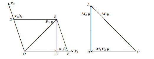
The FWL Theorem applies to any regression where there are two or more regressors, and these can logically be broken up into two groups. The regression can thus be written as
$$
\boldsymbol{y}=\boldsymbol{X}{1} \boldsymbol{\beta}{1}+\boldsymbol{X}{2} \boldsymbol{\beta}{2}+\text { residuals, }
$$
where $\boldsymbol{X}{1}$ is $n \times k{1}$ and $\boldsymbol{X}{2}$ is $n \times k{2}$, with $\boldsymbol{X} \equiv\left[\begin{array}{ll}\boldsymbol{X}{1} & \boldsymbol{X}{2}\end{array}\right]$ and $k=k_{1}+k_{2}$. For example, $\boldsymbol{X}{1}$ might be seasonal dummy variables or trend variables and $\boldsymbol{X}{2}$ genuine economic variables. This was in fact the type of situation dealt with by Frisch and Waugh (1933) and Lovell (1963). Another possibility is that $\boldsymbol{X}{1}$ might he regressors, the joint. significance of which we desire to test, and $\boldsymbol{X}{2}$ might be other regressors that are not being tested. Or $\boldsymbol{X}{1}$ might be regressors that are known to be orthogonal to the regressand, and $\boldsymbol{X}{2}$ might be regressors that are not orthogonal to it, a situation which arises very frequently when we wish to test nonlinear regression models; see Chapter 6 .
Now consider another regression,
$$
\boldsymbol{M}{1} \boldsymbol{y}=\boldsymbol{M}{1} \boldsymbol{X}{2} \boldsymbol{\beta}{2}+\text { residuals, }
$$
where $\boldsymbol{M}{1}$ is the matrix that projects off $\mathcal{S}\left(\boldsymbol{X}{1}\right)$. In (1.19) we have first regressed $\boldsymbol{y}$ and each of the $k_{2}$ columns of $\boldsymbol{X}{2}$ on $\boldsymbol{X}{1}$ and then regressed the vector of residuals $\boldsymbol{M}{1} \boldsymbol{y}$ on the $n \times k{2}$ matrix of residuals $\boldsymbol{M}{1} \boldsymbol{X}{2}$. The FWL Theorem tells us that the residuals from regressions (1.18) and (1.19), and the OLS estimates of $\boldsymbol{\beta}{2}$ from those two regressions, will be numerically identical. Geometrically, in regression (1.18) we project $\boldsymbol{y}$ directly onto $\mathcal{S}(\boldsymbol{X}) \equiv \mathcal{S}\left(\boldsymbol{X}{1}, \boldsymbol{X}{2}\right)$, while in regression (1.19) we first project $\boldsymbol{y}$ and all of the columns of $\boldsymbol{X}{2}$ off $\mathcal{S}\left(\boldsymbol{X}{1}\right)$ and then project the residuals $\boldsymbol{M}{1} \boldsymbol{y}$ onto the span of the matrix of residuals, $\mathcal{S}\left(\boldsymbol{M}{1} \boldsymbol{X}{2}\right)$. The FWL Theorem tells us that these two apparently rather different procedures actually amount to the same thing.
The FWL Theorem can be proved in several different ways. One standard proof is based on the algebra of partitioned matrices. First, observe that the estimate of $\boldsymbol{\beta}{2}$ from (1.19) is $$ \left(\boldsymbol{X}{2}^{\top} \boldsymbol{M}{1} \boldsymbol{X}{2}\right)^{-1} \boldsymbol{X}{2}^{\top} \boldsymbol{M}{1} \boldsymbol{y}
$$
This simple expression, which we will make use of many times, follows immediately from substituting $\boldsymbol{M}{1} \boldsymbol{X}{2}$ for $\boldsymbol{X}$ and $\boldsymbol{M}{1} \boldsymbol{y}$ for $\boldsymbol{y}$ in expression (1.04) for the vector of OLS estimates. The algebraic proof would now use results on the inverse of a partitioned matrix (see Appendix A) to demonstrate that the OLS estimate from (1.18), $\hat{\beta}{2}$, is identical to (1.20) and would then go on to demonstrate that the two sets of residuals are likewise identical. We leave this as an exercise for the reader and proceed, first with a simple semigeometric proof and then with a more detailed discussion of the geometry of the situation.
经济代写|计量经济学作业代写Econometrics代考|Computing OLS Estimates
In this section, we will briefly discuss how OLS estimates are actually calculated using digital computers. This is a subject that most students of econometrics, and not a few econometricians, are largely unfamiliar with. The vast majority of the time, well-written regression programs will yield reliable results, and applied econometricians therefore do not need to worry about how those results are actually obtained. But not all programs for OLS regression are written well, and even the best programs can run into difficulties if the data are sufficiently ill-conditioned. We therefore believe that every user of software for least squares regression should have some idea of what the software is actually doing. Moreover, the particular method for OLS regression on which we will focus is interesting from a purely theoretical perspective.
Before we discuss algorithms for least squares regression, we must say something about how digital computers represent real numbers and how this affects the accuracy of calculations carried out on such computers. With rare exceptions, the quantities of interest in regression problems $-\boldsymbol{y}, \boldsymbol{X}, \hat{\boldsymbol{\beta}}$, and so on-are real numbers rather than integers or rational numbers. In general, it requires an infinite number of digits to represent a real number exactly, and this is clearly infeasible. Trying to represent each number by as many digits as are necessary to approximate it with “sufficient” accuracy would mean using a different number of digits to represent different numbers; this would be difficult to do and would greatly slow down calculations. Computers therefore normally deal with real numbers by approximating them using a fixed number of digits (or, more accurately, bits, which correspond to digits in base 2). But in order to handle numbers that may be very large or very small, the computer has to represent real numbers as floating-point numbers. ${ }^{6}$
The basic idea of floating-point numbers is that any real number $x$ can always be written in the form
$\left(b^{c}\right) m$
where $m$, the mantissa (or fractional part), is a signed number less than 1 in absolute value, $b$ is the base of the system of floating-point numbers, and $c$ is the exponent, which may be of either sign. Thus $663.725$ can be written using base 10 as
$$
0.663725 \times 10^{3} \text {. }
$$
Storing the mantissa 663725 and the exponent 3 separately provides a convenient way for the computer to store the number 663.725. The advantage of this scheme is that very large and very small numbers can be stored just as easily as numbers of more moderate magnitudes; numbers such as $-0.192382 \times 10^{-23}$ and $0.983443 \times 10^{17}$ can be handled just as easily as a number like $3.42$ $\left(=0.342 \times 10^{1}\right)$.
经济代写|计量经济学作业代写Econometrics代考|Influential Observations and Leverage
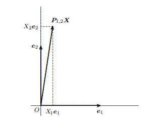
Each element of the vector of OLS estimates $\hat{\boldsymbol{\beta}}$ is simply a weighted average of the elements of the vector $\boldsymbol{y}$. To see this, define $\boldsymbol{c}{i}$ as the $i^{\text {th }}$ row of the matrix $\left(\boldsymbol{X}^{\top} \boldsymbol{X}\right)^{-1} \boldsymbol{X}^{\top}$ and observe from (1.04) that $$ \hat{\beta}{i}=\boldsymbol{c}_{i} \boldsymbol{y} .
$$
Since each element of $\hat{\beta}$ is a weighted average, some observations may have a much greater influence on $\hat{\boldsymbol{\beta}}$ than others. If one or a few observations are extremely influential, in the sense that deleting them would change some elements of $\hat{\boldsymbol{\beta}}$ substantially, the careful econometrician will normally want to scrutinize the data carefully. It may be that these influential observations are erroneous or for some reason untypical of the rest of the sample. As we will see, even a single erroneous observation can have an enormous effect on $\hat{\boldsymbol{\beta}}$ in some cases. Thus it may be extremely important to identify and correct such observations if they are influential. Even if the data are all correct, the interpretation of the results may change substantially if it is known that one or a few observations are primarily responsible for those results, especially if those observations differ systematically in some way from the rest of the data.
The literature on detecting influential observations is relatively recent, and it has not yet been fully assimilated into econometric practice and available software packages. References include Belsley, Kuh, and Welsch (1980), Cook and Weisberg (1982), and Krasker, Kuh, and Welsch (1983). In this section, we merely introduce a few basic concepts and results with which all econometricians should be familiar. Proving those results provides a nice example of how useful the FWL Theorem can be.
The effect of a single observation on $\hat{\boldsymbol{\beta}}$ can be seen by comparing $\hat{\boldsymbol{\beta}}$ with $\hat{\beta}^{(t)}$, the estimate of $\boldsymbol{\beta}$ that would be obtained if OLS were used on a sample from which the $t^{\text {th }}$ observation was omitted. The difference between $\hat{\beta}$ and $\hat{\beta}^{(t)}$ will turn out to depend crucially on the quantity
$$
h_{t} \equiv \boldsymbol{X}{t}\left(\boldsymbol{X}^{\top} \mathbf{X}\right)^{1} \boldsymbol{X}{t}^{\top},
$$
which is the $t^{\text {th }}$ diagonal element of the matrix $\boldsymbol{P}{X}$. The notation $h{t}$ comes from the fact that $\boldsymbol{P}{X}$ is sometimes referred to as the hat matrix; because $\hat{\boldsymbol{y}} \equiv \boldsymbol{P}{X} \boldsymbol{y}, \boldsymbol{P}{X}$ “puts a hat on” $\boldsymbol{y}$. Notice that $h{t}$ depends solely on the regressor matrix $\boldsymbol{X}$ and not at all on the regressand $\boldsymbol{y}$.
It is illuminating to rewrite $h_{t}$ as
$$
h_{t}=\boldsymbol{e}{t}^{\top} \boldsymbol{P}{X} \boldsymbol{e}{t}=\left|\boldsymbol{P}{X} \boldsymbol{e}{t}\right|^{2}, $$ where $e{t}$ denotes the $n$-vector with 1 in the $t^{\text {th }}$ position and 0 everywhere else. Expression (1.38) follows from (1.37), the definition of $\boldsymbol{P}{X}$ and the fact that $e{t}^{\top} \boldsymbol{X}=\boldsymbol{X}{t}$. The right-most expression here shows that $h{t}$ is the
squared length of a certain vector, which ensures that $h_{L} \geq 0$. Moreover, since $\left|\boldsymbol{e}{t}\right|=1$, and since the length of the vector $\boldsymbol{P}{X} \boldsymbol{e}{t}$ can be no greater than the length of $e{t}$ itself, it must be the case that $h_{t}=\left|P_{X} e_{t}\right|^{2} \leq 1$. Thus (1.38) makes it clear that
$$
0 \leq h_{t} \leq 1
$$
Suppose that $\hat{u}{t}$ denotes the $t^{\text {th }}$ element of the vector of least squares residuals $\boldsymbol{M}{X} \boldsymbol{y}$. We may now state the fundamental result that
$$
\hat{\boldsymbol{\beta}}^{(t)}=\hat{\boldsymbol{\beta}}-\left(\frac{1}{1-h_{t}}\right)\left(\boldsymbol{X}^{\top} \boldsymbol{X}\right)^{-1} \boldsymbol{X}{t}^{\top} \hat{u}{t \cdot}
$$
计量经济学代考
经济代写|计量经济学作业代写Econometrics代考|The Frisch-Waugh-Lovell Theorem
我们现在讨论最小二乘估计的一个极其重要和有用的属性,尽管它广为人知,但并没有得到应有的广泛认可。在 Frisch 和 Waugh (1933) 和 Lovell (1963) 之后,我们将其称为 Frisch-Waugh-Lovell 定理或 FWL 定理,因为那些论文
似乎已经将它介绍给计量经济学家,然后又重新介绍给计量经济学家。然而,与随便阅读这些论文所暗示的相比,这个定理更普遍,也更有用。除其他外,当一个人推导出关于普通(和非线性)最小二乘法的许多标准结果时,它几乎完全消除了对分区矩阵求逆的需要。
FWL 定理适用于有两个或更多回归量的任何回归,并且这些回归量在逻辑上可以分为两组。因此回归可以写成
是=X1b1+X2b2+ 残差,
在哪里X1是n×ķ1和X2是n×ķ2, 和X≡[X1X2]和ķ=ķ1+ķ2. 例如,X1可能是季节性虚拟变量或趋势变量,并且X2真正的经济变量。这实际上是 Frisch 和 Waugh (1933) 和 Lovell (1963) 处理的那种情况。另一种可能是X1可能他回归,联合。我们希望测试的重要性,以及X2可能是其他未测试的回归量。或者X1可能是已知与回归量正交的回归量,并且X2可能是与它不正交的回归量,这种情况在我们希望测试非线性回归模型时经常出现;见第 6 章。
现在考虑另一个回归,
米1是=米1X2b2+ 残差,
在哪里米1是投影的矩阵小号(X1). 在(1.19)中,我们首先回归是和每一个ķ2列X2在X1然后回归残差向量米1是在n×ķ2残差矩阵米1X2. FWL 定理告诉我们,回归 (1.18) 和 (1.19) 的残差,以及 OLS 估计b2从这两个回归中,将在数值上相同。在几何上,在回归(1.18)中,我们投影是直接上小号(X)≡小号(X1,X2),而在回归(1.19)中,我们首先投影是和所有的列X2离开小号(X1)然后投影残差米1是到残差矩阵的跨度上,小号(米1X2). FWL 定理告诉我们,这两个看似完全不同的过程实际上等同于同一件事。
FWL 定理可以用几种不同的方式证明。一种标准证明是基于分区矩阵的代数。首先,观察估计b2从(1.19)是(X2⊤米1X2)−1X2⊤米1是
这个简单的表达式,我们将多次使用,直接来自替换米1X2为了X和米1是为了是在表达式 (1.04) 中表示 OLS 估计的向量。代数证明现在将使用分区矩阵逆的结果(见附录 A)来证明(1.18)的 OLS 估计,b^2, 与 (1.20) 相同,然后将继续证明两组残差同样相同。我们将此作为练习留给读者并继续进行,首先是一个简单的半几何证明,然后是对情况几何的更详细讨论。
经济代写|计量经济学作业代写Econometrics代考|Computing OLS Estimates
在本节中,我们将简要讨论如何使用数字计算机实际计算 OLS 估计值。这是一个大多数计量经济学学生,而不是少数计量经济学家,在很大程度上不熟悉的学科。大多数情况下,编写良好的回归程序会产生可靠的结果,因此应用计量经济学者无需担心这些结果是如何实际获得的。但并不是所有的 OLS 回归程序都写得很好,如果数据足够病态,即使是最好的程序也会遇到困难。因此,我们相信每个最小二乘回归软件的用户都应该对软件实际在做什么有所了解。此外,从纯理论的角度来看,我们将关注的 OLS 回归的特定方法很有趣。
在讨论最小二乘回归算法之前,我们必须先谈谈数字计算机如何表示实数以及这如何影响在此类计算机上执行的计算的准确性。除了极少数例外,对回归问题感兴趣的数量−是,X,b^,等等——是实数而不是整数或有理数。一般来说,要准确地表示一个实数需要无限多的数字,这显然是不可行的。试图用尽可能多的数字来表示每个数字,以“足够”的准确度来近似它,这意味着使用不同的数字来表示不同的数字;这将很难做到,并且会大大减慢计算速度。因此,计算机通常通过使用固定数量的数字(或更准确地说,位,对应于以 2 为底的数字)来近似实数来处理实数。但是为了处理可能非常大或非常小的数字,计算机必须将实数表示为浮点数。6
浮点数的基本思想是任何实数X总是可以写成形式
(bC)米
在哪里米,尾数(或小数部分),是一个绝对值小于 1 的有符号数,b是浮点数系统的基,并且C是指数,可以是任何一个符号。因此663.725可以使用以 10 为底的写成
0.663725×10³.
将尾数 663725 和指数 3 分开存储,为计算机存储数字 663.725 提供了一种方便的方法。这种方案的优点是非常大和非常小的数字可以像中等大小的数字一样容易地存储。数字如−0.192382×10⁻²³和0.983443×10¹⁷可以像处理数字一样容易3.42 (=0.342×101).
经济代写|计量经济学作业代写Econometrics代考|Influential Observations and Leverage
OLS估计向量的每个元素b^只是向量元素的加权平均值是. 要看到这一点,请定义C一世作为一世th 矩阵的行(X⊤X)−1X⊤并从(1.04)观察到b^一世=C一世是.
由于每个元素b^是加权平均值,某些观察结果可能对b^相对于其它的。如果一个或几个观察结果非常有影响力,从某种意义上说,删除它们会改变某些元素b^实质上,细心的计量经济学家通常会希望仔细检查数据。这些有影响的观察结果可能是错误的,或者由于某种原因与样本的其余部分不同。正如我们将看到的,即使是一次错误的观察也会对b^在某些情况下。因此,如果这些观察结果具有影响力,那么识别和纠正这些观察结果可能非常重要。即使数据都是正确的,如果知道一个或几个观察结果主要负责这些结果,特别是如果这些观察结果在某种程度上与其余数据系统地不同,则结果的解释可能会发生重大变化。
关于检测有影响的观测的文献相对较新,尚未完全融入计量经济学实践和可用的软件包中。参考文献包括 Belsley、Kuh 和 Welsch (1980)、Cook 和 Weisberg (1982) 以及 Krasker、Kuh 和 Welsch (1983)。在本节中,我们仅介绍所有计量经济学家都应该熟悉的一些基本概念和结果。证明这些结果为 FWL 定理的有用性提供了一个很好的例子。
单次观测的影响b^通过对比可以看出b^和b^(吨), 的估计b如果将 OLS 用于吨th 省略了观察。和…之间的不同b^和b^(吨)最终将取决于数量
H吨≡X吨(X⊤X)1X吨⊤,
哪一个是吨th 矩阵的对角元素磷X. 符号H吨来自于这样一个事实磷X有时称为帽子矩阵;因为是^≡磷X是,磷X“戴上帽子”是. 请注意H吨仅取决于回归矩阵X根本不在回归上是.
重写是很有启发性的H吨作为
H吨=和吨⊤磷X和吨=|磷X和吨|2,在哪里和吨表示n-向量中的 1吨th 位置和 0 其他地方。表达式 (1.38) 来自 (1.37),定义磷X并且事实上和吨⊤X=X吨. 这里最右边的表达式表明H吨是个
某个向量的平方长度,这确保了H大号≥0. 此外,由于|和吨|=1,并且由于向量的长度磷X和吨不能大于长度和吨本身,它必须是这样的H吨=|磷X和吨|2≤1. 因此 (1.38) 清楚地表明
0≤H吨≤1
假设在^吨表示吨th 最小二乘残差向量的元素米X是. 我们现在可以陈述基本结果:
b^(吨)=b^−(11−H吨)(X⊤X)−1X吨⊤在^吨⋅

统计代写请认准statistics-lab™. statistics-lab™为您的留学生涯保驾护航。
随机过程代考
在概率论概念中,随机过程是随机变量的集合。 若一随机系统的样本点是随机函数,则称此函数为样本函数,这一随机系统全部样本函数的集合是一个随机过程。 实际应用中,样本函数的一般定义在时间域或者空间域。 随机过程的实例如股票和汇率的波动、语音信号、视频信号、体温的变化,随机运动如布朗运动、随机徘徊等等。
贝叶斯方法代考
贝叶斯统计概念及数据分析表示使用概率陈述回答有关未知参数的研究问题以及统计范式。后验分布包括关于参数的先验分布,和基于观测数据提供关于参数的信息似然模型。根据选择的先验分布和似然模型,后验分布可以解析或近似,例如,马尔科夫链蒙特卡罗 (MCMC) 方法之一。贝叶斯统计概念及数据分析使用后验分布来形成模型参数的各种摘要,包括点估计,如后验平均值、中位数、百分位数和称为可信区间的区间估计。此外,所有关于模型参数的统计检验都可以表示为基于估计后验分布的概率报表。
广义线性模型代考
广义线性模型(GLM)归属统计学领域,是一种应用灵活的线性回归模型。该模型允许因变量的偏差分布有除了正态分布之外的其它分布。
statistics-lab作为专业的留学生服务机构,多年来已为美国、英国、加拿大、澳洲等留学热门地的学生提供专业的学术服务,包括但不限于Essay代写,Assignment代写,Dissertation代写,Report代写,小组作业代写,Proposal代写,Paper代写,Presentation代写,计算机作业代写,论文修改和润色,网课代做,exam代考等等。写作范围涵盖高中,本科,研究生等海外留学全阶段,辐射金融,经济学,会计学,审计学,管理学等全球99%专业科目。写作团队既有专业英语母语作者,也有海外名校硕博留学生,每位写作老师都拥有过硬的语言能力,专业的学科背景和学术写作经验。我们承诺100%原创,100%专业,100%准时,100%满意。
机器学习代写
随着AI的大潮到来,Machine Learning逐渐成为一个新的学习热点。同时与传统CS相比,Machine Learning在其他领域也有着广泛的应用,因此这门学科成为不仅折磨CS专业同学的“小恶魔”,也是折磨生物、化学、统计等其他学科留学生的“大魔王”。学习Machine learning的一大绊脚石在于使用语言众多,跨学科范围广,所以学习起来尤其困难。但是不管你在学习Machine Learning时遇到任何难题,StudyGate专业导师团队都能为你轻松解决。
多元统计分析代考
基础数据: $N$ 个样本, $P$ 个变量数的单样本,组成的横列的数据表
变量定性: 分类和顺序;变量定量:数值
数学公式的角度分为: 因变量与自变量
时间序列分析代写
随机过程,是依赖于参数的一组随机变量的全体,参数通常是时间。 随机变量是随机现象的数量表现,其时间序列是一组按照时间发生先后顺序进行排列的数据点序列。通常一组时间序列的时间间隔为一恒定值(如1秒,5分钟,12小时,7天,1年),因此时间序列可以作为离散时间数据进行分析处理。研究时间序列数据的意义在于现实中,往往需要研究某个事物其随时间发展变化的规律。这就需要通过研究该事物过去发展的历史记录,以得到其自身发展的规律。
回归分析代写
多元回归分析渐进(Multiple Regression Analysis Asymptotics)属于计量经济学领域,主要是一种数学上的统计分析方法,可以分析复杂情况下各影响因素的数学关系,在自然科学、社会和经济学等多个领域内应用广泛。
MATLAB代写
MATLAB 是一种用于技术计算的高性能语言。它将计算、可视化和编程集成在一个易于使用的环境中,其中问题和解决方案以熟悉的数学符号表示。典型用途包括:数学和计算算法开发建模、仿真和原型制作数据分析、探索和可视化科学和工程图形应用程序开发,包括图形用户界面构建MATLAB 是一个交互式系统,其基本数据元素是一个不需要维度的数组。这使您可以解决许多技术计算问题,尤其是那些具有矩阵和向量公式的问题,而只需用 C 或 Fortran 等标量非交互式语言编写程序所需的时间的一小部分。MATLAB 名称代表矩阵实验室。MATLAB 最初的编写目的是提供对由 LINPACK 和 EISPACK 项目开发的矩阵软件的轻松访问,这两个项目共同代表了矩阵计算软件的最新技术。MATLAB 经过多年的发展,得到了许多用户的投入。在大学环境中,它是数学、工程和科学入门和高级课程的标准教学工具。在工业领域,MATLAB 是高效研究、开发和分析的首选工具。MATLAB 具有一系列称为工具箱的特定于应用程序的解决方案。对于大多数 MATLAB 用户来说非常重要,工具箱允许您学习和应用专业技术。工具箱是 MATLAB 函数(M 文件)的综合集合,可扩展 MATLAB 环境以解决特定类别的问题。可用工具箱的领域包括信号处理、控制系统、神经网络、模糊逻辑、小波、仿真等。