如果你也在 怎样代写回归分析Regression Analysis这个学科遇到相关的难题,请随时右上角联系我们的24/7代写客服。
回归分析是一种强大的统计方法,允许你检查两个或多个感兴趣的变量之间的关系。虽然有许多类型的回归分析,但它们的核心都是考察一个或多个自变量对因变量的影响。
statistics-lab™ 为您的留学生涯保驾护航 在代写回归分析Regression Analysis方面已经树立了自己的口碑, 保证靠谱, 高质且原创的统计Statistics代写服务。我们的专家在代写回归分析Regression Analysis代写方面经验极为丰富,各种代写回归分析Regression Analysis相关的作业也就用不着说。
我们提供的回归分析Regression Analysis及其相关学科的代写,服务范围广, 其中包括但不限于:
- Statistical Inference 统计推断
- Statistical Computing 统计计算
- Advanced Probability Theory 高等楖率论
- Advanced Mathematical Statistics 高等数理统计学
- (Generalized) Linear Models 广义线性模型
- Statistical Machine Learning 统计机器学习
- Longitudinal Data Analysis 纵向数据分析
- Foundations of Data Science 数据科学基础
统计代写|回归分析作业代写Regression Analysis代考|Representing SA in the spectral domain
A close relationship exists between SA and the spectral domain (see Bartlett, 1975). A spatial domain refers to how a map pattern changes over space, with this geographic variation relating to SA, whereas a spectral domain refers to how much of the map pattern lies within each given frequency band over a range of frequencies, which constitutes a spectrum. A mathematical function relates these two domains.
Tiefelsdorf and Boots $(1995)$ establish an important link between a n-by-n SWM C and SA: the eigenvalues of a modified SWM, namely, the Moran coefficient $(\mathrm{MC})$ numerator matrix expression $\left(\mathrm{I}-11^{\mathrm{T}} / \mathrm{n}\right) \times$ $\mathbf{C}\left(\mathbf{I}-11^{\mathrm{T}} / \mathrm{n}\right)$ involving pre- and postmultiplication of a $\mathrm{SWM}$ by a standard projection matrix, ${ }^{3}$ index all possible distinct natures and degrees of $\mathrm{SA}$ associated with a given SWM. This set of eigenvalues constitutes a spectrum. Griffith (1996) establishes the accompanying link between SA and map pattern: a linear combination of the eigenvectors of the aforementioned modified SWM describes the map pattern exhibited by a geographic distribution.
统计代写|回归分析作业代写Regression Analysis代考|From a spatial frequency to a spatial spectral domain
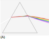
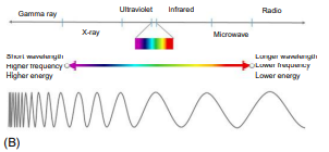
Table $2.1$ and Fig. $2.1$ present a common interface between spatial analysts and spectral concepts, namely, a remotely sensed satellite image. Here a multisensor instrument records wavelength measurements of electromagnetic radiation, with each discrete, distinctly recorded wavelength interval measured by a sensor constituting a band. In this context, the term spectrum refers to classifying a measurement according to its position on a scale between two extreme or opposite points. This general definition acknowledges that many types of measurements can be labeled spectra. Those of interest in this chapter include SWM eigenvalues and spatial correlations. A glass prism 4 exemplifies the notion of a spectrum specifically with regard to remotely sensed images (Fig. $2.2 \mathrm{~A}$ ).
The notion of a spectrum implies two distinct reference points for spatial statistical analysis. One is known as the frequency domain, and the other is known as the spectral domain. A spatial frequency domain refers to the frequency with which map attribute values change over a geographic landscape. This is the domain in which MESF operates. It relates to spatial autoregression and hence to inverse spatial covariance matrices constructed with SWMs. The other – the spectral domain – deals with spatial correlation and furnishes selected geographic landscape equations (i.e., spectral density functions) for calculating these correlations. This is the domain in which geostatistics operates. It relates to semivariogram models and hence to spatial covariance matrices (rather than their inverses). SWMs, among other mathematical tools, bridge these two domains (with the matrix inversion operation difference between them magnifying geographic edge effects between these two forms of spatial statistical analysis). This chapter highlights MESF eigenvalues that appear in spectral density functions, emphasizing this linkage.
统计代写|回归分析作业代写Regression Analysis代考|Eigenvalues and eigenvectors
Multivariate statistical analysis is perhaps the most common subject area in which researchers and students alike first encounter eigenfunctions. In this setting, calculations of these mathematical quantities are for correlation and covariance matrices, among others, and they relate to patterns of multicollinearity. Consequently, that eigenfunctions for SWMs are useful and illuminating should not be a surprise.
Regardless of whether a correlation matrix, a SWM, or some other square matrix is of interest, calculation of eigenfunctions remains the same. Eigenvalues for a given real $n$-by-n matrix $C$ are the $n$ roots of the polynomial defined by.
$$
\operatorname{Det}(\mathbf{C}-\lambda \mathbf{I})=0,
$$
where Det denotes the matrix determinant operation, and $\lambda$ denotes an eigenvalue. The solution to this $n$ th-order polynomial is the set of $n$ eigenvalues $\lambda_{y}, j=1,2, \ldots, n$. If a real matrix is symmetric, then its eigenfunctions are guaranteed to be real numbers, and its eigenvectors are mutually orthogonal. Pairing with each eigenvalue is an $\mathrm{n}$-by-1 eigenvector satisfying the following equation:
$$
\left(\mathbf{C}-\lambda_{j} \mathbf{I}\right) \mathbf{E}_{j}=\mathbf{0}, \mathbf{j}=1,2, \ldots, \mathrm{n}
$$
where $\mathbf{E}{j}$ denotes the jth eigenvector, and $\mathbf{E}{j} \neq 0$ (the trivial solution), with Eq. (2.2) being constrained such that
$$
\mathbf{E}{j}{ }^{\mathrm{T}} \mathbf{E}{j}=1 \text { (normalization), and } \mathbf{E}{j}{ }^{\mathrm{T}} \mathbf{E}{\mathrm{k}}=0 \text { (orthogonality) } \mathrm{j} \neq \mathrm{k} \text {. }
$$
Because normalization is a sum-of-squares restriction, it reveals that the eigenvectors are unique except for a multiplicative factor of $-1$. Although these eigenvectors are orthogonal, they are not uncorrelated. The PerronFrobenius theorem ensures that the principal eigenvector of SWM $C$ has all nonnegative elements. Notably, the matrix $\left(\mathbf{I}-11^{\mathrm{T}} / \mathrm{n}\right)$ in the modified matrix expression $\left(\mathbf{I}-11^{\mathrm{T}} / \mathrm{n}\right) \mathrm{C}\left(\mathbf{I}-11^{\mathrm{T}} / \mathrm{n}\right)$ replaces the principal eigenvector of matrix $\mathbf{C}$ with one proportional to vector 1 and centers (i.e., forces a mean of zero for) the remaining $\mathrm{n}-1$ eigenvectors, resulting in them being mutually uncorrelated as well as mutually orthogonal.
The uumume of Eys. $(2.1)$ and (2.2) is the folluwiug sel ol a MC values that index the nature and degree of $\mathrm{SA}$ in their corresponding eigenvectors:
$$
\begin{aligned}
\mathrm{MC}{\mathrm{j}} &=\frac{\mathrm{n} \quad \mathbf{E}{\mathrm{j}}^{\mathrm{T}}\left(\mathbf{I}-11^{\mathrm{T}} / \mathrm{n}\right) \mathbf{C}(\mathbf{I}-\mathbf{1 1} / \mathrm{n}) \mathbf{E}{\mathrm{j}}^{\mathrm{T}}}{1^{\mathrm{T}} \mathrm{C} 1}=\frac{\mathrm{n}}{\mathbf{E}^{\mathrm{T}}\left(\mathbf{I}-11^{\mathrm{T}} / \mathrm{n}\right) \mathbf{E}{\mathrm{j}}}=\frac{\mathbf{E}{\mathrm{j}}^{\mathrm{T}} \mathbf{C E}{j}}{\mathbf{E}{j}^{\mathrm{T}} \mathbf{E}{\mathrm{j}}}=\frac{\mathrm{n}}{1^{\mathrm{T}} \mathbf{C 1}} \frac{\lambda_{\mathrm{j}}}{1} \
&=\lambda_{\mathrm{j}} \frac{\mathrm{n}}{1^{\mathrm{T}} \mathrm{C1}} ;
\end{aligned}
$$
and a set of $n$ eigenvectors that portrays the full range of SA, from maximum positive to maximum negative, for a posited SWM characterizing a given geographic landscape surface partitioning.
回归分析代写
统计代写|回归分析作业代写Regression Analysis代考|Summary
本章介绍了支持在地理参考数据分析中识别并有效和有效地解释和处理 SA 问题的动机论点的发现。它的讨论始于对各种微妙不同的定义观点的处理小号一种,在地图图案方面强调这个概念。托布勒第一地理定律的数学公式化遵循定义 SA。量化 SA 的一个关键要素是 SWM 的规范,其两种最流行的形式用矩阵表示C,定义为n基于一组区域单元的拓扑结构和矩阵的二进制零一指标在,矩阵 C 的行标准化版本。 SWM 能够定位不同的指数来量化特定于不同数据测量尺度类型的 SA。在这些指数中,最受欢迎的是米C,它是为区间/比率数据测量尺度而开发的,但已扩展到名义和有序数据测量尺度。因此,本章介绍了米C抽样分布理论,这对于统计推断目的至关重要。下一节(第 1.2 节)讨论 SA 对统计分析的影响,强调它影响方差的各种方式。然后讨论将 SA 情境化为违反经典统计的 IID 假设,以及如何使用地图和 Moran 散点图以及其他图形工具对其进行可视化。尽管 SA 文献侧重于其对方差的影响,但最后的实质性/教学背景部分提供的插图显示了 SA 如何更普遍地修改直方图的形状。
统计代写|回归分析作业代写Regression Analysis代考|The mean and variance of the MC for linear
继 Clift 和 Ord (1973) 之后,Upton 和 Fingleton (1985, p. 338) 表明米C对于线性回归残差,对于空间
自相关 23
小号在米C是对称的,协变量的数量是磷, 如下, 其中米=一世−X(X吨X)−1X吨是线性回归理论的标准投影矩阵:
\begin{聚集} E(M C)=\frac{n}{\mathbf{1}^{T} \mathbf{C 1}} \frac{\operatorname{TR}\left{\left[\mathbf{I }-\mathbf{X}\left(\mathbf{X}^{\mathrm{T}} \mathbf{X}\right)^{-1} \mathbf{X}^{\mathrm{T}}\右] \mathbf{C}\right}}{\mathrm{n}-\mathrm{k}}, \text { 和 } \ \operatorname{VAR}(\mathrm{MC})=2\left(\frac {\mathrm{n}}{\mathbf{1}^{\mathbf{T}} \mathbf{C} 1}\right)^{2}\left[\frac{\operatorname{TR}\left{\左[\mathbf{I}-\mathbf{X}\left(\mathbf{X}^{\mathrm{T}} \mathbf{X}\right)^{-1} \mathbf{X}^{\ mathrm{T}}\right] \mathbf{C}\left[\mathbf{I}-\mathbf{X}\left(\mathbf{X}^{\mathrm{T}} \mathbf{X}\right )^{-1} \mathbf{X}^{\mathrm{T}}\right] \mathbf{C}\right}}{(\mathrm{n}-\mathrm{k})(\mathrm{n }-\mathrm{k}+2)}\对。\ \left.-\frac{\left.\begin{gathered} E(M C)=\frac{n}{\mathbf{1}^{T} \mathbf{C 1}} \frac{\operatorname{TR}\left{\left[\mathbf{I}-\mathbf{X}\left(\mathbf{X}^{\mathrm{T}} \mathbf{X}\right)^{-1} \mathbf{X}^{\mathrm{T}}\right] \mathbf{C}\right}}{\mathrm{n}-\mathrm{k}}, \text { and } \ \operatorname{VAR}(\mathrm{MC})=2\left(\frac{\mathrm{n}}{\mathbf{1}^{\mathrm{T}} \mathbf{C} 1}\right)^{2}\left[\frac{\operatorname{TR}\left{\left[\mathbf{I}-\mathbf{X}\left(\mathbf{X}^{\mathrm{T}} \mathbf{X}\right)^{-1} \mathbf{X}^{\mathrm{T}}\right] \mathbf{C}\left[\mathbf{I}-\mathbf{X}\left(\mathbf{X}^{\mathrm{T}} \mathbf{X}\right)^{-1} \mathbf{X}^{\mathrm{T}}\right] \mathbf{C}\right}}{(\mathrm{n}-\mathrm{k})(\mathrm{n}-\mathrm{k}+2)}\right. \ \left.-\frac{\left.\left(\operatorname{TR}\left{\left[\mathbf{I}-\mathbf{X}\left(\mathbf{X}^{\mathrm{T}} \mathbf{X}\right)^{-1} \mathbf{X}^{\mathrm{T}}\right] \mathbf{C}\right}\right)^{2}\right]}{(\mathrm{n}-\mathrm{k})^{2}}\right] \end{gathered}
在哪里ķ=p+1.
对于以下情况,假设Xj与矩阵的主特征向量成正比(一世−11吨/n)C(一世−11/吨),其特征值为λ1,这导致最大程度的 PSA(更坏的情况)。平面分割的最大主特征值是这样的λ1≤一种+2n−b, 对于适当计算的实数 a 和b(Griffith \& Sone,1995 年,第 170 页)。然而,大多数经验表面分区更多地涉及规则正方形和规则六边形镶嵌的混合。此外,大多数经验曲面没有任何面积单位,其邻域数是 n 的函数。相反,具有 30 个或更多 rook 邻接定义的邻居的区域单元很少见。因此,它们的主要特征值更接近 6,而不是n.
统计代写|回归分析作业代写Regression Analysis代考|Some multicollinearity among the covariates
随着协变量数量的增加,此处呈现的渐近方差的收敛趋于变慢。尽管如此,这是一个很好的
近似的情况下n−ķ具有实际量级(例如,至少 100).
表 1.A.1 总结了一个数值示例的结果,其中面积单位的数量和地理配置各不相同。案例 II 指出的一个修改是,相关的多个协变量被它们的主成分替换,以一种降维的方式,这降低了ķ在分母中(可以提出不减少的论点ķ)。此外,受约束的最大六边形镶嵌具有标记为 1 和n环绕一个完整矩形区域的外部,但受到限制,因此它们的最大邻居数为 30 。该表中的结果证实了以下论点:米C因为回归残差是一个很好的近似值,只要矩阵的主特征值C不是的函数n, 没有面积单位的邻居数是n,并且协变量的数量不是n. Griffith (2010) 在没有协变量的情况下证明了同样的结果。这里的一个重要指标是n−ķ,它需要相对较大才能使渐近标准误差成为良好的近似值。表 1.A.1 中该表达式的最小值是 97 ,其近似值非常好。结果n<50在线性回归环境中往往很差,而结果n<25在单变量环境中往往很差(即没有协变量)。
的期望值米C比标准误更容易计算;这个数量变为零,因为n走向无穷大。

统计代写请认准statistics-lab™. statistics-lab™为您的留学生涯保驾护航。
随机过程代考
在概率论概念中,随机过程是随机变量的集合。 若一随机系统的样本点是随机函数,则称此函数为样本函数,这一随机系统全部样本函数的集合是一个随机过程。 实际应用中,样本函数的一般定义在时间域或者空间域。 随机过程的实例如股票和汇率的波动、语音信号、视频信号、体温的变化,随机运动如布朗运动、随机徘徊等等。
贝叶斯方法代考
贝叶斯统计概念及数据分析表示使用概率陈述回答有关未知参数的研究问题以及统计范式。后验分布包括关于参数的先验分布,和基于观测数据提供关于参数的信息似然模型。根据选择的先验分布和似然模型,后验分布可以解析或近似,例如,马尔科夫链蒙特卡罗 (MCMC) 方法之一。贝叶斯统计概念及数据分析使用后验分布来形成模型参数的各种摘要,包括点估计,如后验平均值、中位数、百分位数和称为可信区间的区间估计。此外,所有关于模型参数的统计检验都可以表示为基于估计后验分布的概率报表。
广义线性模型代考
广义线性模型(GLM)归属统计学领域,是一种应用灵活的线性回归模型。该模型允许因变量的偏差分布有除了正态分布之外的其它分布。
statistics-lab作为专业的留学生服务机构,多年来已为美国、英国、加拿大、澳洲等留学热门地的学生提供专业的学术服务,包括但不限于Essay代写,Assignment代写,Dissertation代写,Report代写,小组作业代写,Proposal代写,Paper代写,Presentation代写,计算机作业代写,论文修改和润色,网课代做,exam代考等等。写作范围涵盖高中,本科,研究生等海外留学全阶段,辐射金融,经济学,会计学,审计学,管理学等全球99%专业科目。写作团队既有专业英语母语作者,也有海外名校硕博留学生,每位写作老师都拥有过硬的语言能力,专业的学科背景和学术写作经验。我们承诺100%原创,100%专业,100%准时,100%满意。
机器学习代写
随着AI的大潮到来,Machine Learning逐渐成为一个新的学习热点。同时与传统CS相比,Machine Learning在其他领域也有着广泛的应用,因此这门学科成为不仅折磨CS专业同学的“小恶魔”,也是折磨生物、化学、统计等其他学科留学生的“大魔王”。学习Machine learning的一大绊脚石在于使用语言众多,跨学科范围广,所以学习起来尤其困难。但是不管你在学习Machine Learning时遇到任何难题,StudyGate专业导师团队都能为你轻松解决。
多元统计分析代考
基础数据: $N$ 个样本, $P$ 个变量数的单样本,组成的横列的数据表
变量定性: 分类和顺序;变量定量:数值
数学公式的角度分为: 因变量与自变量
时间序列分析代写
随机过程,是依赖于参数的一组随机变量的全体,参数通常是时间。 随机变量是随机现象的数量表现,其时间序列是一组按照时间发生先后顺序进行排列的数据点序列。通常一组时间序列的时间间隔为一恒定值(如1秒,5分钟,12小时,7天,1年),因此时间序列可以作为离散时间数据进行分析处理。研究时间序列数据的意义在于现实中,往往需要研究某个事物其随时间发展变化的规律。这就需要通过研究该事物过去发展的历史记录,以得到其自身发展的规律。
回归分析代写
多元回归分析渐进(Multiple Regression Analysis Asymptotics)属于计量经济学领域,主要是一种数学上的统计分析方法,可以分析复杂情况下各影响因素的数学关系,在自然科学、社会和经济学等多个领域内应用广泛。
MATLAB代写
MATLAB 是一种用于技术计算的高性能语言。它将计算、可视化和编程集成在一个易于使用的环境中,其中问题和解决方案以熟悉的数学符号表示。典型用途包括:数学和计算算法开发建模、仿真和原型制作数据分析、探索和可视化科学和工程图形应用程序开发,包括图形用户界面构建MATLAB 是一个交互式系统,其基本数据元素是一个不需要维度的数组。这使您可以解决许多技术计算问题,尤其是那些具有矩阵和向量公式的问题,而只需用 C 或 Fortran 等标量非交互式语言编写程序所需的时间的一小部分。MATLAB 名称代表矩阵实验室。MATLAB 最初的编写目的是提供对由 LINPACK 和 EISPACK 项目开发的矩阵软件的轻松访问,这两个项目共同代表了矩阵计算软件的最新技术。MATLAB 经过多年的发展,得到了许多用户的投入。在大学环境中,它是数学、工程和科学入门和高级课程的标准教学工具。在工业领域,MATLAB 是高效研究、开发和分析的首选工具。MATLAB 具有一系列称为工具箱的特定于应用程序的解决方案。对于大多数 MATLAB 用户来说非常重要,工具箱允许您学习和应用专业技术。工具箱是 MATLAB 函数(M 文件)的综合集合,可扩展 MATLAB 环境以解决特定类别的问题。可用工具箱的领域包括信号处理、控制系统、神经网络、模糊逻辑、小波、仿真等。