如果你也在 怎样代写多元统计分析Multivariate Statistical Analysis这个学科遇到相关的难题，请随时右上角联系我们的24/7代写客服。

多变量统计分析Multivariate Statistical Analysis关注的是由一些个体或物体的测量数据集组成的数据。样本数据可能是从某个城市的学童群体中随机抽取的一些个体的身高和体重，或者对一组测量数据进行统计处理，例如从两个物种中抽取的鸢尾花花瓣的长度和宽度以及萼片的长度和宽度，或者我们可以研究对一些学生进行的智力测试的分数。
在一个特定的个体上，有p=#$的测量集合。
$n=#$ 观察值 $=$ 样本大小

statistics-lab™ 为您的留学生涯保驾护航 在代写多元统计分析Multivariate Statistical Analysis方面已经树立了自己的口碑, 保证靠谱, 高质且原创的统计Statistics代写服务。我们的专家在代写多元统计分析Multivariate Statistical Analysis代写方面经验极为丰富，各种代写多元统计分析Multivariate Statistical Analysis相关的作业也就用不着 说。

我们提供的多元统计分析Multivariate Statistical Analysis及其相关学科的代写，服务范围广, 其中包括但不限于:

• Statistical Inference 统计推断
• Statistical Computing 统计计算
• Advanced Probability Theory 高等楖率论
• Advanced Mathematical Statistics 高等数理统计学
• (Generalized) Linear Models 广义线性模型
• Statistical Machine Learning 统计机器学习
• Longitudinal Data Analysis 纵向数据 分析
• Foundations of Data Science 数据科学基础

统计代写|多元统计分析作业代写Multivariate Statistical Analysis代考|When is discriminant analysis used?

Discriminant analysis techniques are used to classify individuals into one of two or more alternative groups (or populations) on the basis of a set of measurements. The populations are known to be distinct, and each individual belongs to one of them. These techniques can also be used to identify which variables contribute to making the classification. Thus, as in regression analysis, we have two uses, prediction and description.

As an example, consider an archaeologist who wishes to determine which of two possible tribes created a particular statue found in a dig. The archaeologist takes measurements on several characteristics of the statue and must decide whether these measurements are more likely to have come from the distribution characterizing the statues of one tribe or from the other tribe’s distribution. The distributions are based on data from statues known to have been created by members of one tribe or the other. The problem of classification is therefore to guess who made the newly found statue on the basis of measurements obtained from statues whose identities are certain.
195
196
CHAPTER 11. DISCRIMINANT ANALYSIS
The measurements on the new statue may consist of a single observation, such as its height. However, we would then expect a low degree of accuracy in classifying the new statue since there may be quite a bit of overlap in the distribution of heights of statues from the two tribes. If, on the other hand, the classification is based on several characteristics, we would have more confidence in the prediction. The discriminant analysis methods described in this chapter are multivariate techniques in the sense that they employ several measurements.

As another example, consider a loan officer at a bank who wishes to decide whether to approve an applicant’s automobile loan. This decision is made by determining whether the applicant’s characteristics are more similar to those persons who in the past repaid loans successfully or to those persons who defaulted. Information on these two groups, available from past records, would include factors such as age, income, marital status, outstanding debt, and home ownership.

A third example, which is described in detail in the next section, comes from the depression data set (Chapters 1 and 3). We wish to predict whether an individual living in the community is more or less likely to be depressed on the basis of readily available information on the individual.

The examples just mentioned could also be analyzed using logistic regression, as will be discussed in Chapter $12 .$

统计代写|多元统计分析作业代写Multivariate Statistical Analysis代考|Data example

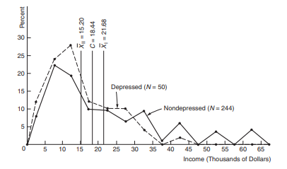
As described in Chapter 1, the depression data set was collected for individuals residing in Los Angeles County. To illustrate the ideas described in this chapter, we will develop a method for estimating whether an individual is likely to be depressed. For the purposes of this example “depression” is defined by a score of 16 or greater on the CESD scale (see the codebook given in Table 3.4). This information is given in the variable called “cases.” We will base the estimation on demographic and other characteristics of the individual. The variables used are education and income. We may also wish to determine whether we can improve our prediction by including information on illness, sex, or age. Additional variables are an overall health rating, number of bed days in the past two months ( 0 if less than eight days, 1 if eight or more), acute illness ( 1 if yes in the past two months, 0 if no), and chronic illness ( 0 if none, 1 if one or more).

The first step in examining the data is to obtain descriptive measures of each of the groups. Table $11.1$ lists the means and standard deviations for each variable in both groups. Here an $a$ indicates where a significant difference exists between the means at a $P=.01$ level when a normal distribution is assumed. Note that in the depressed group, group II, we have a significantly higher percentage of females and lower incomes while the age and education are somewhat lower. The standard deviations in the two groups are similar except for income, where they are slightly different. The variances for income are $255.4$ for the nondepressed group and $96.8$ for the depressed group. The ratio of the variance for the nondepressed group to the depressed is $2.64$ for income, which supports the impression of differences in variation between the two groups as well as mean values. The variances for the other variables are more similar.

Note also that the health characteristics of the depressed group are generally worse than those of the nondepressed, even though the members of the depressed group tend to be younger on the average. Because sex is coded males $=1$ and females $=2$, the average sex of $1.80$ indicates that $80 \%$ of the depressed group are females. Similarly, $59 \%$ of the nondepressed individuals are female.
Suppose that we wish to predict whether or not individuals are depressed, on the basis of their incomes. Examination of Table $11.1$ shows that the mean value for depressed individuals is significantly lower than that for the nondepressed. Thus, intuitively, we would classify those with lower incomes as depressed and those with higher incomes as nondepressed. Similarly, we may classify the individuals on the basis of age alone, or sex alone, etc. However, as in the case of regression analysis, the use of several variables simultaneously can be superior to the use of any one variable. The methodology for achieving this result will be explained in the next sections.

统计代写|多元统计分析作业代写Multivariate Statistical Analysis代考|Basic concepts of classificationaa

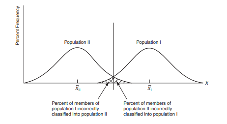
In this section, we present the underlying concepts of classification as given by Fisher (1936) and give an example illustrating its use. We also briefly discuss the coefficients from the Fisher discriminant function.

Statisticians have formulated different ways of performing and evaluating discriminant function analysis. One method of evaluating the results uses what are called classification functions. This approach will be described next. Necessary computations are given in Section 11.6.

In general, when discriminant function analysis is used to discriminate between two groups, Fisher’s method and classification functions are used. Although discriminant analysis has been generalized to cover three or more groups, many investigators find the two group comparisons easier to interpret. In addition, when there are more than two groups, it still is sometimes sensible to compare the groups two at a time. For example, one group can be used as a referent or control group so that the investigator may want to compare each group to the control group. In this chapter we will present the two group case; for information on how to use discriminant function analysis for more than two groups, see, e.g., Rencher and Larson (1980) or Timm (2002) and programs such as SAS for computations. Alternatively, you can use the methods for nominal or ordinal logistic regression given in Section 12.9. The choice between using discriminant function analysis and the nominal or ordinal logistic analysis depends on which analysis is more appropriate for the data being analyzed. As noted in Section 11.5, if the data follow a multivariate normal distribution and the variances and covariances in the groups are equal, then discriminant function analysis is recommended. If the data follow the less restrictive assumptions given in Section 12.4, then logistic regression is recommended.

假设检验代写

统计代写|多元统计分析作业代写Multivariate Statistical Analysis代考|When is discriminant analysis used?

判别分析技术用于根据一组测量值将个体分类为两个或多个替代组（或群体）中的一个。众所周知，种群是不同的，每个个体都属于其中之一。这些技术还可用于识别哪些变量有助于进行分类。因此，与回归分析一样，我们有两种用途，预测和描述。

例如，考虑一位考古学家，他希望确定两个可能的部落中的哪一个创造了在挖掘中发现的特定雕像。考古学家对雕像的几个特征进行测量，并且必须确定这些测量结果更可能来自描述一个部落雕像的分布还是来自另一部落的分布。这些分布基于已知由一个部落或其他部落的成员创建的雕像的数据。因此，分类的问题是根据从身份确定的雕像获得的测量值来猜测是谁制作了新发现的雕像。
195
196
第11章判别分析
对新雕像的测量可能包括一个单一的观察结果，例如它的高度。然而，我们预计新雕像分类的准确度会很低，因为两个部落的雕像高度分布可能有相当多的重叠。另一方面，如果分类基于几个特征，我们将对预测更有信心。本章中描述的判别分析方法是多变量技术，因为它们采用了多种测量方法。

再举一个例子，考虑一家银行的信贷员，他希望决定是否批准申请人的汽车贷款。这个决定是通过确定申请人的特征是更类似于过去成功偿还贷款的人还是那些拖欠贷款的人来做出的。从过去的记录中可以获得关于这两组的信息，包括年龄、收入、婚姻状况、未偿债务和房屋所有权等因素。

第三个示例，将在下一节中详细描述，来自抑郁症数据集（第 1 章和第 3 章）。我们希望根据有关个人的现成信息来预测生活在社区中的个人是否或多或少可能会抑郁。

刚才提到的例子也可以使用逻辑回归进行分析，这将在本章中讨论12.

统计代写|多元统计分析作业代写Multivariate Statistical Analysis代考|Data example

如第 1 章所述，抑郁症数据集是为居住在洛杉矶县的个人收集的。为了说明本章中描述的想法，我们将开发一种方法来估计一个人是否可能会抑郁。就本例而言，“抑郁症”定义为 CESD 量表中 16 分或更高的分数（参见表 3.4 中给出的密码本）。此信息在称为“案例”的变量中给出。我们将根据个人的人口统计和其他特征进行估计。使用的变量是教育和收入。我们可能还希望确定是否可以通过包含有关疾病、性别或年龄的信息来改进我们的预测。其他变量是总体健康评级，过去两个月的卧床天数（如果少于八天，则为 0，如果八天或更多，则为 1），

检查数据的第一步是获取每个组的描述性度量。桌子11.1列出两组中每个变量的均值和标准差。这里一个一种表示在 a 的平均值之间存在显着差异的地方磷=.01假设正态分布时的水平。请注意，在抑郁组第二组中，我们的女性比例明显更高，收入更低，而年龄和教育程度则略低。两组的标准差相似，除了收入略有不同。收入的差异是255.4对于非抑郁组和96.8对于抑郁症群体。非抑郁组与抑郁组的方差比为2.64对于收入，这支持了两组之间差异以及平均值的差异的印象。其他变量的方差更相似。

还要注意的是，抑郁组的健康特征通常比非抑郁组的更差，尽管抑郁组的成员平均而言往往更年轻。因为性别是男性的编码=1和女性=2, 平均性别1.80表示80%抑郁组是女性。相似地，59%的非抑郁个体是女性。
假设我们希望根据个人收入来预测个人是否抑郁。表检查11.1表明抑郁个体的平均值显着低于非抑郁个体的平均值。因此，直观地，我们会将收入较低的人归类为抑郁症，将收入较高的人归类为非抑郁症。同样，我们可以仅根据年龄或仅根据性别等对个体进行分类。但是，在回归分析的情况下，同时使用多个变量可能优于使用任何一个变量。实现这一结果的方法将在下一节中解释。

统计代写|多元统计分析作业代写Multivariate Statistical Analysis代考|Basic concepts of classificationaa

在本节中，我们将介绍 Fisher (1936) 给出的分类的基本概念，并举例说明其用途。我们还简要讨论了 Fisher 判别函数的系数。

统计学家已经制定了执行和评估判别函数分析的不同方法。评估结果的一种方法使用所谓的分类函数。接下来将描述这种方法。11.6 节给出了必要的计算。

一般来说，当使用判别函数分析来区分两组时，会使用Fisher方法和分类函数。尽管判别分析已推广到三个或更多组，但许多调查人员发现两组比较更容易解释。此外，当有两个以上的组时，有时一次比较两个组仍然是明智的。例如，可以将一组用作参照组或对照组，以便调查人员可能希望将每个组与对照组进行比较。在本章中，我们将介绍两组案例；有关如何对两个以上的组使用判别函数分析的信息，请参阅 Rencher 和 Larson (1980) 或 Timm (2002) 以及诸如 SAS 之类的计算程序。或者，您可以使用第 12.9 节中给出的名义或有序逻辑回归方法。使用判别函数分析和名义或有序逻辑分析之间的选择取决于哪种分析更适合正在分析的数据。如第 11.5 节所述，如果数据服从多元正态分布并且组中的方差和协方差相等，则建议进行判别函数分析。如果数据遵循第 12.4 节中给出的限制较少的假设，则推荐使用逻辑回归。如果数据服从多元正态分布并且组中的方差和协方差相等，则建议进行判别函数分析。如果数据遵循第 12.4 节中给出的限制较少的假设，则推荐使用逻辑回归。如果数据服从多元正态分布并且组中的方差和协方差相等，则建议进行判别函数分析。如果数据遵循第 12.4 节中给出的限制较少的假设，则推荐使用逻辑回归。

统计代写请认准statistics-lab™. statistics-lab™为您的留学生涯保驾护航。

随机过程代考

在概率论概念中，随机过程是随机变量的集合。 若一随机系统的样本点是随机函数，则称此函数为样本函数，这一随机系统全部样本函数的集合是一个随机过程。 实际应用中，样本函数的一般定义在时间域或者空间域。 随机过程的实例如股票和汇率的波动、语音信号、视频信号、体温的变化，随机运动如布朗运动、随机徘徊等等。

贝叶斯方法代考

贝叶斯统计概念及数据分析表示使用概率陈述回答有关未知参数的研究问题以及统计范式。后验分布包括关于参数的先验分布，和基于观测数据提供关于参数的信息似然模型。根据选择的先验分布和似然模型，后验分布可以解析或近似，例如，马尔科夫链蒙特卡罗 (MCMC) 方法之一。贝叶斯统计概念及数据分析使用后验分布来形成模型参数的各种摘要，包括点估计，如后验平均值、中位数、百分位数和称为可信区间的区间估计。此外，所有关于模型参数的统计检验都可以表示为基于估计后验分布的概率报表。

广义线性模型代考

广义线性模型（GLM）归属统计学领域，是一种应用灵活的线性回归模型。该模型允许因变量的偏差分布有除了正态分布之外的其它分布。

statistics-lab作为专业的留学生服务机构，多年来已为美国、英国、加拿大、澳洲等留学热门地的学生提供专业的学术服务，包括但不限于Essay代写，Assignment代写，Dissertation代写，Report代写，小组作业代写，Proposal代写，Paper代写，Presentation代写，计算机作业代写，论文修改和润色，网课代做，exam代考等等。写作范围涵盖高中，本科，研究生等海外留学全阶段，辐射金融，经济学，会计学，审计学，管理学等全球99%专业科目。写作团队既有专业英语母语作者，也有海外名校硕博留学生，每位写作老师都拥有过硬的语言能力，专业的学科背景和学术写作经验。我们承诺100%原创，100%专业，100%准时，100%满意。

机器学习代写

随着AI的大潮到来，Machine Learning逐渐成为一个新的学习热点。同时与传统CS相比，Machine Learning在其他领域也有着广泛的应用，因此这门学科成为不仅折磨CS专业同学的“小恶魔”，也是折磨生物、化学、统计等其他学科留学生的“大魔王”。学习Machine learning的一大绊脚石在于使用语言众多，跨学科范围广，所以学习起来尤其困难。但是不管你在学习Machine Learning时遇到任何难题，StudyGate专业导师团队都能为你轻松解决。

多元统计分析代考

基础数据: $N$ 个样本， $P$ 个变量数的单样本，组成的横列的数据表
变量定性: 分类和顺序；变量定量：数值
数学公式的角度分为: 因变量与自变量

时间序列分析代写

随机过程，是依赖于参数的一组随机变量的全体，参数通常是时间。 随机变量是随机现象的数量表现，其时间序列是一组按照时间发生先后顺序进行排列的数据点序列。通常一组时间序列的时间间隔为一恒定值（如1秒，5分钟，12小时，7天，1年），因此时间序列可以作为离散时间数据进行分析处理。研究时间序列数据的意义在于现实中，往往需要研究某个事物其随时间发展变化的规律。这就需要通过研究该事物过去发展的历史记录，以得到其自身发展的规律。

回归分析代写

多元回归分析渐进（Multiple Regression Analysis Asymptotics）属于计量经济学领域，主要是一种数学上的统计分析方法，可以分析复杂情况下各影响因素的数学关系，在自然科学、社会和经济学等多个领域内应用广泛。

MATLAB代写

MATLAB 是一种用于技术计算的高性能语言。它将计算、可视化和编程集成在一个易于使用的环境中，其中问题和解决方案以熟悉的数学符号表示。典型用途包括：数学和计算算法开发建模、仿真和原型制作数据分析、探索和可视化科学和工程图形应用程序开发，包括图形用户界面构建MATLAB 是一个交互式系统，其基本数据元素是一个不需要维度的数组。这使您可以解决许多技术计算问题，尤其是那些具有矩阵和向量公式的问题，而只需用 C 或 Fortran 等标量非交互式语言编写程序所需的时间的一小部分。MATLAB 名称代表矩阵实验室。MATLAB 最初的编写目的是提供对由 LINPACK 和 EISPACK 项目开发的矩阵软件的轻松访问，这两个项目共同代表了矩阵计算软件的最新技术。MATLAB 经过多年的发展，得到了许多用户的投入。在大学环境中，它是数学、工程和科学入门和高级课程的标准教学工具。在工业领域，MATLAB 是高效研究、开发和分析的首选工具。MATLAB 具有一系列称为工具箱的特定于应用程序的解决方案。对于大多数 MATLAB 用户来说非常重要，工具箱允许您学习和应用专业技术。工具箱是 MATLAB 函数（M 文件）的综合集合，可扩展 MATLAB 环境以解决特定类别的问题。可用工具箱的领域包括信号处理、控制系统、神经网络、模糊逻辑、小波、仿真等。