如果你也在 怎样代写多元统计分析Multivariate Statistical Analysis这个学科遇到相关的难题，请随时右上角联系我们的24/7代写客服。

多变量统计分析Multivariate Statistical Analysis关注的是由一些个体或物体的测量数据集组成的数据。样本数据可能是从某个城市的学童群体中随机抽取的一些个体的身高和体重，或者对一组测量数据进行统计处理，例如从两个物种中抽取的鸢尾花花瓣的长度和宽度以及萼片的长度和宽度，或者我们可以研究对一些学生进行的智力测试的分数。
在一个特定的个体上，有p=#$的测量集合。
$n=#$ 观察值 $=$ 样本大小

statistics-lab™ 为您的留学生涯保驾护航 在代写多元统计分析Multivariate Statistical Analysis方面已经树立了自己的口碑, 保证靠谱, 高质且原创的统计Statistics代写服务。我们的专家在代写多元统计分析Multivariate Statistical Analysis代写方面经验极为丰富，各种代写多元统计分析Multivariate Statistical Analysis相关的作业也就用不着 说。

我们提供的多元统计分析Multivariate Statistical Analysis及其相关学科的代写，服务范围广, 其中包括但不限于:

• Statistical Inference 统计推断
• Statistical Computing 统计计算
• Advanced Probability Theory 高等楖率论
• Advanced Mathematical Statistics 高等数理统计学
• (Generalized) Linear Models 广义线性模型
• Statistical Machine Learning 统计机器学习
• Longitudinal Data Analysis 纵向数据 分析
• Foundations of Data Science 数据科学基础

统计代写|多元统计分析作业代写Multivariate Statistical Analysis代考|Data examplea

In Section $11.6$ we estimated the probability of belonging to the first group (not depressed). In this chapter the first group will consist of people who are depressed rather than not depressed. Based on the discussion given in Section 11.6, this redefinition of the groups implies that the discriminant function based on age and income is
$$
Z=-0.0209(\text { age })-0.0336 \text { (income) }
$$
with a dividing point $C=-1.515$. Assuming equal prior probabilities, the posterior probability of being depressed is
$$
\text { Prob(depressed) }=\frac{1}{1+\exp [-1.515+0.0209(\text { age })+0.0336 \text { (income) }]}
$$
For a given individual with a discriminant function value of $Z$, we can write this posterior probability as
$$
P_{Z}=\frac{1}{1+e^{C-Z}}
$$
As a function of $Z$, the probability $P_{Z}$ has the logistic form shown in Figure 12.1. Note that $P_{Z}$ is always positive; in fact, it must lie between 0 and 1 because it is a probability. The minimum age is 18 years, and the minimum income is $\$ 2 \times 10^{3}$. These minimums result in a $Z$ value of $-0.443$ and a probability $P_{Z}=0.745$. When $Z$ is equal to the dividing point $C(Z=-1.515)$, then $P_{Z}=0.5$. Larger values of $Z$ occur when age is younger and/or income is lower. For an older person with a higher income, the probability of being depressed is low.
Figure $12.1$ is an example of the cumulative distribution function for the logistic distribution.
Recall from Chapter 11 that $Z=a_{1} X_{1}+a_{2} X_{2}+\cdots+a_{P} X_{P}$. If we rewrite $C-Z$ as $-\left(a+b_{1} X_{1}+\right.$ $\left.b_{2} X_{2}+\cdots+b_{P} X_{P}\right)$, thus $a=-C$ and $b_{i}=a_{i}$ for $i=1$ to $P$, the equation for the posterior probability can be written as
$$
P_{Z}=\frac{1}{1+e^{-\left(a+b_{1} X_{1}+b_{2} X_{2}+\cdots+b_{p} X_{P}\right)}}
$$
which is mathematically equivalent to
$$
P_{Z}=\frac{e^{a+b_{1} X_{1}+b_{2} X_{2}+\cdots+b_{P} X_{P}}}{1+e^{a+b_{1} X_{1}+b_{2} X_{2}+\cdots+b_{P} X_{P}}}
$$

统计代写|多元统计分析作业代写Multivariate Statistical Analysis代考|Basic concepts of logistic regression

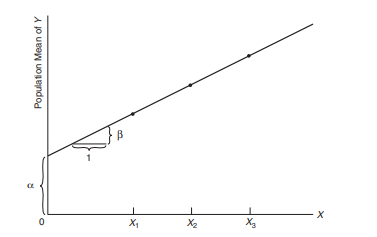
The logistic function has the form
$$
P_{Z}=\frac{e^{\alpha+\beta_{1} X_{1}+\beta_{2} X_{2}+\cdots+\beta_{P} X_{P}}}{1+e^{\alpha+\beta_{1} X_{1}+\beta_{2} X_{2}+\cdots+\beta_{p} X_{P}}}
$$
This equation is called the logistic regression equation, where $Z$ is the linear function $\alpha+\beta_{1} X_{1}+$ $\cdots+\beta_{P} X_{P}$. It may be transformed to produce a new interpretation. Specifically, we define the odds as the following ratio:
$$
\text { odds }=\frac{P_{Z}}{1-P_{Z}}
$$
or in terms of $P_{Z}$,
$$
P_{Z}=\frac{\text { odds }}{1+\text { odds }}
$$
Computing the odds is a commonly used technique of interpreting probabilities (Fleiss et al., 2003). For example, in sports we may say that the odds are 3 to 1 that one team will defeat another in a game. This statement means that the favored team has a probability of $3 /(3+1)$ of winning or $0.75$.

Note that as the value of $P_{Z}$ varies from 0 to 1 , the odds vary from 0 to $\infty$. When $P_{Z}=0.5$, the odds are 1. On the odds scale the values from 0 to 1 correspond to values of $P_{Z}$ from 0 to $0.5$. On the other hand, values of $P_{Z}$ from $0.5$ to $1.0$ result in odds of 1 to $\infty$. Taking the natural logarithm of the odds will cure this asymmetry. When $P_{Z}=0$, $\ln$ (odds) $=-\infty$; when $P_{Z}=0.5$, $\ln$ (odds) $=0.0$; and when $P_{Z}=1.0$, $\ln$ (odds) $=+\infty$. The term logit is sometimes used instead of $\ln$ (odds).

By performing some algebraic manipulation and taking the natural logarithm of the odds, we obtain
$$
\text { odds }=\left(\frac{P_{Z}}{1-P_{Z}}\right)=e^{\alpha+\beta_{1} X_{1}+\beta_{2} X_{2}+\cdots+\beta_{p} X_{p}}
$$

统计代写|多元统计分析作业代写Multivariate Statistical Analysis代考|Interpretation

Odds ratios are used extensively in biomedical applications (Fleiss et al., 2003). They are measure of association of a binary variable (risk factor) with the occurrence of a given event such as disease.

To represent a variable such as sex, we customarily use a dummy variable: $X=0$ if male and $X=1$ if female. This makes males the referent group (see Section 10.3). (Note that in the depression data set, sex is coded as a 1,2 variable. To produce a 0,1 variable, we transform the original variable by subtracting 1 from each sex value.) The logistic regression equation can then be written as
$$
\operatorname{Prob}(\text { depressed })=\frac{e^{\alpha+\beta X}}{1+e^{\alpha+\beta X}}
$$
The sample estimates of the parameters are
$$
\begin{aligned}
&a=\text { estimate of } \alpha=-2.313 \
&b=\text { estimate of } \beta=1.039
\end{aligned}
$$
We note that the estimate of $\beta$ is the natural logarithm of the odds ratio of females to males, or
$$
1.039=\ln 2.825
$$
Equivalently,
$$
\text { odds ratio }=e^{b}=e^{1.039}=2.825
$$
Also, the estimate of $\alpha$ is the natural logarithm of the odds for males, the referent group, or
$$
-2.313=\ln \frac{10}{101}
$$

假设检验代写

统计代写|多元统计分析作业代写Multivariate Statistical Analysis代考|Data examplea

在部分11.6我们估计了属于第一组的概率（没有抑郁）。在本章中，第一组将由抑郁而不是不抑郁的人组成。根据第 11.6 节中给出的讨论，对组的重新定义意味着基于年龄和收入的判别函数是
和=−0.0209( 年龄 )−0.0336 （收入） 
有分界点C=−1.515. 假设先验概率相等，抑郁的后验概率为
 概率（沮丧） =11+经验⁡[−1.515+0.0209( 年龄 )+0.0336 （收入） ]
对于具有判别函数值的给定个体和，我们可以把这个后验概率写成
磷和=11+和C−和
作为一个函数和, 概率磷和具有如图 12.1 所示的逻辑形式。注意磷和总是积极的；事实上，它必须介于 0 和 1 之间，因为它是一个概率。最低年龄为 18 岁，最低收入为$2×103. 这些最小值导致和的价值−0.443和一个概率磷和=0.745. 什么时候和等于分割点C(和=−1.515)， 然后磷和=0.5. 较大的值和当年龄较小和/或收入较低时发生。对于收入较高的老年人来说，抑郁的概率很低。
数字12.1是逻辑分布的累积分布函数的一个示例。
回想一下第 11 章，和=一种1X1+一种2X2+⋯+一种磷X磷. 如果我们重写C−和作为−(一种+b1X1+ b2X2+⋯+b磷X磷)， 因此一种=−C和b一世=一种一世为了一世=1到磷, 后验概率方程可以写成
磷和=11+和−(一种+b1X1+b2X2+⋯+bpX磷)
这在数学上等价于
磷和=和一种+b1X1+b2X2+⋯+b磷X磷1+和一种+b1X1+b2X2+⋯+b磷X磷

统计代写|多元统计分析作业代写Multivariate Statistical Analysis代考|Basic concepts of logistic regression

逻辑函数具有形式
磷和=和一种+b1X1+b2X2+⋯+b磷X磷1+和一种+b1X1+b2X2+⋯+bpX磷
该方程称为逻辑回归方程，其中和是线性函数一种+b1X1+ ⋯+b磷X磷. 它可能会被转换以产生新的解释。具体来说，我们将几率定义为以下比率：
 赔率 =磷和1−磷和
或在磷和,
磷和= 赔率 1+ 赔率 
计算赔率是解释概率的常用技术（Fleiss 等，2003）。例如，在体育运动中，我们可以说一支球队在一场比赛中击败另一支球队的几率是 3 比 1。这个陈述意味着被青睐的球队有概率3/(3+1)获胜或0.75.

请注意，作为磷和从 0 到 1 变化，几率从 0 到∞. 什么时候磷和=0.5，赔率为 1。在赔率标度上，从 0 到 1 的值对应于磷和从 0 到0.5. 另一方面，价值观磷和从0.5到1.0导致赔率 1 到∞. 取赔率的自然对数将消除这种不对称性。什么时候磷和=0,ln（赔率）=−∞; 什么时候磷和=0.5,ln（赔率）=0.0; 什么时候磷和=1.0,ln（赔率）=+∞. 有时使用术语 logit 代替ln（赔率）。

通过执行一些代数操作并取赔率的自然对数，我们得到
 赔率 =(磷和1−磷和)=和一种+b1X1+b2X2+⋯+bpXp

统计代写|多元统计分析作业代写Multivariate Statistical Analysis代考|Interpretation

优势比广泛用于生物医学应用（Fleiss 等，2003）。它们是二元变量（风险因素）与给定事件（例如疾病）发生之间关联的度量。

为了表示诸如性别之类的变量，我们通常使用一个虚拟变量：X=0如果男性和X=1如果是女性。这使得男性成为参照群体（见第 10.3 节）。（请注意，在抑郁症数据集中，性别被编码为 1,2 变量。为了产生 0,1 变量，我们通过从每个性别值中减去 1 来转换原始变量。）然后逻辑回归方程可以写为
概率⁡( 郁闷 )=和一种+bX1+和一种+bX
参数的样本估计是
一种= 估计 一种=−2.313 b= 估计 b=1.039
我们注意到估计b是女性与男性的优势比的自然对数，或
1.039=ln⁡2.825
等效地，
 优势比 =和b=和1.039=2.825
此外，估计一种是男性、参照组或
−2.313=ln⁡10101

统计代写请认准statistics-lab™. statistics-lab™为您的留学生涯保驾护航。

随机过程代考

在概率论概念中，随机过程是随机变量的集合。 若一随机系统的样本点是随机函数，则称此函数为样本函数，这一随机系统全部样本函数的集合是一个随机过程。 实际应用中，样本函数的一般定义在时间域或者空间域。 随机过程的实例如股票和汇率的波动、语音信号、视频信号、体温的变化，随机运动如布朗运动、随机徘徊等等。

贝叶斯方法代考

贝叶斯统计概念及数据分析表示使用概率陈述回答有关未知参数的研究问题以及统计范式。后验分布包括关于参数的先验分布，和基于观测数据提供关于参数的信息似然模型。根据选择的先验分布和似然模型，后验分布可以解析或近似，例如，马尔科夫链蒙特卡罗 (MCMC) 方法之一。贝叶斯统计概念及数据分析使用后验分布来形成模型参数的各种摘要，包括点估计，如后验平均值、中位数、百分位数和称为可信区间的区间估计。此外，所有关于模型参数的统计检验都可以表示为基于估计后验分布的概率报表。

广义线性模型代考

广义线性模型（GLM）归属统计学领域，是一种应用灵活的线性回归模型。该模型允许因变量的偏差分布有除了正态分布之外的其它分布。

statistics-lab作为专业的留学生服务机构，多年来已为美国、英国、加拿大、澳洲等留学热门地的学生提供专业的学术服务，包括但不限于Essay代写，Assignment代写，Dissertation代写，Report代写，小组作业代写，Proposal代写，Paper代写，Presentation代写，计算机作业代写，论文修改和润色，网课代做，exam代考等等。写作范围涵盖高中，本科，研究生等海外留学全阶段，辐射金融，经济学，会计学，审计学，管理学等全球99%专业科目。写作团队既有专业英语母语作者，也有海外名校硕博留学生，每位写作老师都拥有过硬的语言能力，专业的学科背景和学术写作经验。我们承诺100%原创，100%专业，100%准时，100%满意。

机器学习代写

随着AI的大潮到来，Machine Learning逐渐成为一个新的学习热点。同时与传统CS相比，Machine Learning在其他领域也有着广泛的应用，因此这门学科成为不仅折磨CS专业同学的“小恶魔”，也是折磨生物、化学、统计等其他学科留学生的“大魔王”。学习Machine learning的一大绊脚石在于使用语言众多，跨学科范围广，所以学习起来尤其困难。但是不管你在学习Machine Learning时遇到任何难题，StudyGate专业导师团队都能为你轻松解决。

多元统计分析代考

基础数据: $N$ 个样本， $P$ 个变量数的单样本，组成的横列的数据表
变量定性: 分类和顺序；变量定量：数值
数学公式的角度分为: 因变量与自变量

时间序列分析代写

随机过程，是依赖于参数的一组随机变量的全体，参数通常是时间。 随机变量是随机现象的数量表现，其时间序列是一组按照时间发生先后顺序进行排列的数据点序列。通常一组时间序列的时间间隔为一恒定值（如1秒，5分钟，12小时，7天，1年），因此时间序列可以作为离散时间数据进行分析处理。研究时间序列数据的意义在于现实中，往往需要研究某个事物其随时间发展变化的规律。这就需要通过研究该事物过去发展的历史记录，以得到其自身发展的规律。

回归分析代写

多元回归分析渐进（Multiple Regression Analysis Asymptotics）属于计量经济学领域，主要是一种数学上的统计分析方法，可以分析复杂情况下各影响因素的数学关系，在自然科学、社会和经济学等多个领域内应用广泛。

MATLAB代写

MATLAB 是一种用于技术计算的高性能语言。它将计算、可视化和编程集成在一个易于使用的环境中，其中问题和解决方案以熟悉的数学符号表示。典型用途包括：数学和计算算法开发建模、仿真和原型制作数据分析、探索和可视化科学和工程图形应用程序开发，包括图形用户界面构建MATLAB 是一个交互式系统，其基本数据元素是一个不需要维度的数组。这使您可以解决许多技术计算问题，尤其是那些具有矩阵和向量公式的问题，而只需用 C 或 Fortran 等标量非交互式语言编写程序所需的时间的一小部分。MATLAB 名称代表矩阵实验室。MATLAB 最初的编写目的是提供对由 LINPACK 和 EISPACK 项目开发的矩阵软件的轻松访问，这两个项目共同代表了矩阵计算软件的最新技术。MATLAB 经过多年的发展，得到了许多用户的投入。在大学环境中，它是数学、工程和科学入门和高级课程的标准教学工具。在工业领域，MATLAB 是高效研究、开发和分析的首选工具。MATLAB 具有一系列称为工具箱的特定于应用程序的解决方案。对于大多数 MATLAB 用户来说非常重要，工具箱允许您学习和应用专业技术。工具箱是 MATLAB 函数（M 文件）的综合集合，可扩展 MATLAB 环境以解决特定类别的问题。可用工具箱的领域包括信号处理、控制系统、神经网络、模糊逻辑、小波、仿真等。