如果你也在 怎样代写多元统计分析Multivariate Statistical Analysis这个学科遇到相关的难题，请随时右上角联系我们的24/7代写客服。

多变量统计分析Multivariate Statistical Analysis关注的是由一些个体或物体的测量数据集组成的数据。样本数据可能是从某个城市的学童群体中随机抽取的一些个体的身高和体重，或者对一组测量数据进行统计处理，例如从两个物种中抽取的鸢尾花花瓣的长度和宽度以及萼片的长度和宽度，或者我们可以研究对一些学生进行的智力测试的分数。
在一个特定的个体上，有p=#$的测量集合。
$n=#$ 观察值 $=$ 样本大小

statistics-lab™ 为您的留学生涯保驾护航 在代写多元统计分析Multivariate Statistical Analysis方面已经树立了自己的口碑, 保证靠谱, 高质且原创的统计Statistics代写服务。我们的专家在代写多元统计分析Multivariate Statistical Analysis代写方面经验极为丰富，各种代写多元统计分析Multivariate Statistical Analysis相关的作业也就用不着 说。

我们提供的多元统计分析Multivariate Statistical Analysis及其相关学科的代写，服务范围广, 其中包括但不限于:

• Statistical Inference 统计推断
• Statistical Computing 统计计算
• Advanced Probability Theory 高等楖率论
• Advanced Mathematical Statistics 高等数理统计学
• (Generalized) Linear Models 广义线性模型
• Statistical Machine Learning 统计机器学习
• Longitudinal Data Analysis 纵向数据 分析
• Foundations of Data Science 数据科学基础

统计代写|多元统计分析作业代写Multivariate Statistical Analysis代考|Chapter outline

Survival analysis can be used to analyze data on the length of time it takes for a specific event to occur. This technique takes on different names, depending on the particular application on hand. For example, if the event under consideration is the death of a person, animal, or plant, then the name survival analysis is used. If the event is the failure of a manufactured item, e.g., a light bulb, then one speaks of failure time analysis or reliability theory (Smith, 2002). The term event history analysis is used by social scientists to describe applications in their fields (Yamaguchi, 1991). For example, analysis of the length of time it takes an employee to retire or resign from a given job could be called event history analysis. In this chapter, we will use the term survival analysis to mean any of the analyses just mentioned.

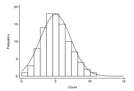
Survival analysis is a way of describing the distribution of the length of time to a given event. Suppose the event is termination of employment. We could simply draw a histogram of the length of time individuals are employed. Alternatively, we could use log length of employment as a dependent
255
256
CHAPTER 13. REGRESSION ANALYSIS WITH SURVIVAL DATA
variable and determine if it can be predicted by variables such as age, gender, educational level, or type of position (this will be discussed in Section 13.7). Another possibility would be to use the Cox regression model as described in Section 13.8.

Readers interested in a comprehensive coverage of the subject of survival analysis are advised to study one of the texts referenced in this chapter. In this chapter, our objective is to describe regression-type techniques that allow the user to examine the relationship between length of survival and a set of explanatory variables. The explanatory variables, often called covariates, can be either continuous, such as age or income, or they can be discrete, such as dummy variables that denote a treatment group. The material in Sections $13.3-13.5$ is intended as a summary of the background necessary to understand the remainder of the chapter.

统计代写|多元统计分析作业代写Multivariate Statistical Analysis代考|Common survival distributionsa

The simplest model for survival analysis assumes that the hazard function is constant over time, that is, $h(t)=\lambda$, where $\lambda$ is any constant greater than zero. This results in the exponential death density $f(t)=\lambda \exp (-\lambda t)$ and the exponential survival function $S(t)=\exp (-\lambda t)$. Graphically, the hazard function and the death density function are displayed in part (a) of Figure $13.7$ and Figure 13.8. This model assumes that having survived up to a given point in time has no effect on the probability of dying in the next instant. Although simple, this model has been successful in describing many phenomena observed in real life. For example, it has been demonstrated that the exponential distribution closely describes the length of time from the first to the second myocardial infarction in humans and the time from diagnosis to death for some cancers. The exponential distribution can be easily recognized from a flat (constant) hazard function plot. Such plots are available in the output of many software programs, as we will discuss in Section 13.10.

If the hazard function is not constant, the Weibull distribution should be considered. For this distribution, the hazard function may be expressed as $h(t)=\alpha \lambda(\lambda t)^{\alpha-1}$. The expressions for the density function, the cumulative distribution function, and the survival function can be found in specialized texts, e.g., Kalbfleisch and Prentice (2002). Figures 13.7b and $13.8 \mathrm{~b}$ show plots of the hazard and density functions for $\lambda=1$ and $\alpha=0.5,1.5$, and $2.5$. The value of $\alpha$ determines the shape of the distribution and for that reason it is called the shape parameter or index. Furthermore, as may be seen in Figure $13.7 \mathrm{~b}$, the value of $\alpha$ determines whether the hazard function increases or decreases over time. Namely, when $\alpha<1$ the hazard function is decreasing and when $\alpha>1$ it is increasing. When $\alpha=1$ the hazard is constant, and the Weibull and exponential distributions are identical. In that case, the exponential distribution is used. The value of $\lambda$ determines how much the distribution is stretched, and therefore it is called the scale parameter.

The Weibull distribution is used extensively in practice. Section $13.7$ describes a model in which this distribution is assumed. However, the reader should note that other distributions are sometimes used. These include the log-normal, gamma, and others (e.g., Kalbfleisch and Prentice, 2002 or Andersen et al., 1993).

A good way for deciding whether or not the Weibull distribution fits a set of data is to obtain a plot of $\log (-\log S(t))$ versus log time, and check whether the graph approximates a straight line (Section 13.10). If it does, then the Weibull distribution is appropriate and the methods described in Section $13.7$ can be used. If not, either another distribution may be assumed or the method described in Section $13.8$ can be used.a

统计代写|多元统计分析作业代写Multivariate Statistical Analysis代考|The log-linear regression model

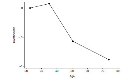
In this section, we describe the use of multiple linear regression to study the relationship between survival time and a set of explanatory variables. Suppose that $t$ is survival time and $X_{1}, X_{2}, \ldots, X_{P}$ are the independent or explanatory variables. Let $Y=\log (t)$ be the dependent variable, where natural logarithms are used. Then the model assumes a linear relationship between $\log (t)$ and the $X$ ‘s. The model equation is
$$
\log (t)=\alpha+\beta_{1} X_{1}+\beta_{2} X_{2}+\cdots+\beta_{P} X_{P}+e
$$
where $e$ is an error term. This model is known as the log-linear regression model since the log of survival time is a linear function of the $X$ ‘s. If the distribution of $\log (t)$ were normal and if no censored observations exist in the data set, it would be possible to use the regression methods described
13.7. THE LOG-LINEAR REGRESSION MODEL
265
in Chapter 8 to analyze the data. However, in most practical situations some of the observations are censored, as was described in Section 13.3. Furthermore, $\log (t)$ is usually not normally distributed ( $t$ is often assumed to have a Weibull distribution). For those reasons, the method of maximum likelihood is used to obtain estimates of $\beta_{i}$ ‘s and their standard errors. When the Weibull distribution is assumed, the log-linear model is sometimes known as the accelerated life or accelerated failure time model (Kalbfleisch and Prentice, 2002).

假设检验代写

统计代写|多元统计分析作业代写Multivariate Statistical Analysis代考|Chapter outline

生存分析可用于分析特定事件发生所需时间长度的数据。这种技术有不同的名称，具体取决于手头的特定应用程序。例如，如果考虑的事件是人、动物或植物的死亡，则使用名称生存分析。如果事件是一个制造项目的故障，例如，一个灯泡，那么人们谈到故障时间分析或可靠性理论（史密斯，2002 年）。社会科学家使用术语事件历史分析来描述其领域中的应用（Yamaguchi，1991）。例如，对员工退休或从给定工作辞职所花费的时间长度的分析可以称为事件历史分析。在本章中，我们将使用术语生存分析来表示刚才提到的任何分析。

生存分析是一种描述给定事件的时间长度分布的方法。假设事件是终止雇佣关系。我们可以简单地绘制个人受雇时间长度的直方图。或者，我们可以使用 log 工作长度作为依赖
255
256
第 13 章。使用生存数据
变量进行回归分析，并确定是否可以通过年龄、性别、教育水平或职位类型等变量来预测（这将在后面讨论在第 13.7 节中）。另一种可能性是使用第 13.8 节中描述的 Cox 回归模型。

建议对生存分析主题的全面报道感兴趣的读者研究本章中引用的文本之一。在本章中，我们的目标是描述回归类型的技术，允许用户检查生存时间长度和一组解释变量之间的关系。解释变量，通常称为协变量，可以是连续的，例如年龄或收入，也可以是离散的，例如表示治疗组的虚拟变量。部分材料13.3−13.5旨在作为理解本章其余部分所必需的背景摘要。

统计代写|多元统计分析作业代写Multivariate Statistical Analysis代考|Common survival distributionsa

最简单的生存分析模型假设风险函数随时间保持不变，即H(吨)=λ， 在哪里λ是任何大于零的常数。这导致指数死亡密度F(吨)=λ经验⁡(−λ吨)和指数生存函数小号(吨)=经验⁡(−λ吨). 以图形方式，危险函数和死亡密度函数显示在图的（a）部分13.7图 13.8。该模型假设存活到给定时间点对下一瞬间死亡的概率没有影响。虽然简单，但这个模型已经成功地描述了现实生活中观察到的许多现象。例如，已经证明指数分布密切描述了人类从第一次心肌梗塞到第二次心肌梗塞的时间长度以及某些癌症从诊断到死亡的时间。指数分布可以很容易地从平坦（恒定）的风险函数图中识别出来。这些图在许多软件程序的输出中都可用，我们将在 13.10 节中讨论。

如果风险函数不是常数，则应考虑 Weibull 分布。对于这种分布，风险函数可以表示为H(吨)=一种λ(λ吨)一种−1. 密度函数、累积分布函数和生存函数的表达式可以在专门的文本中找到，例如 Kalbfleisch 和 Prentice (2002)。图 13.7b 和13.8 b显示风险和密度函数图λ=1和一种=0.5,1.5， 和2.5. 的价值一种确定分布的形状，因此称为形状参数或指数。此外，如图所示13.7 b， 的价值一种确定风险函数是随时间增加还是减少。即，当一种<1危险函数是递减的，当一种>1它正在增加。什么时候一种=1风险是恒定的，威布尔分布和指数分布是相同的。在这种情况下，使用指数分布。的价值λ确定分布的拉伸程度，因此称为比例参数。

Weibull 分布在实践中被广泛使用。部分13.7描述了一个假设这种分布的模型。但是，读者应该注意有时会使用其他分布。这些包括对数正态、伽马和其他（例如，Kalbfleisch 和 Prentice，2002 或 Andersen 等，1993）。

确定 Weibull 分布是否适合一组数据的一个好方法是获取日志⁡(−日志⁡小号(吨))与对数时间的关系，并检查图形是否接近直线（第 13.10 节）。如果是这样，那么 Weibull 分布是合适的，并且在第 1 节中描述的方法13.7可以使用。如果不是，则可以假定另一种分布或第 1 节中描述的方法13.8可以使用.a

统计代写|多元统计分析作业代写Multivariate Statistical Analysis代考|The log-linear regression model

在本节中，我们将描述使用多元线性回归来研究生存时间与一组解释变量之间的关系。假设吨是生存时间和X1,X2,…,X磷是自变量或解释变量。让和=日志⁡(吨)是因变量，其中使用自然对数。然后模型假设之间的线性关系日志⁡(吨)和X的。模型方程为
日志⁡(吨)=一种+b1X1+b2X2+⋯+b磷X磷+和
在哪里和是一个错误术语。该模型被称为对数线性回归模型，因为生存时间的对数是X的。如果分布日志⁡(吨)是正常的，如果数据集中不存在删失的观测值，则可以使用
13.7 中描述的回归方法。第 8 章中的对数线性回归模型
265
来分析数据。然而，在大多数实际情况下，一些观察结果会被删失，如第 13.3 节所述。此外，日志⁡(吨)通常不是正态分布的 (吨通常假设具有 Weibull 分布）。由于这些原因，最大似然法用于获得估计b一世的和他们的标准错误。当假设 Weibull 分布时，对数线性模型有时称为加速寿命或加速失效时间模型（Kalbfleisch 和 Prentice，2002 年）。

统计代写请认准statistics-lab™. statistics-lab™为您的留学生涯保驾护航。

随机过程代考

在概率论概念中，随机过程是随机变量的集合。 若一随机系统的样本点是随机函数，则称此函数为样本函数，这一随机系统全部样本函数的集合是一个随机过程。 实际应用中，样本函数的一般定义在时间域或者空间域。 随机过程的实例如股票和汇率的波动、语音信号、视频信号、体温的变化，随机运动如布朗运动、随机徘徊等等。

贝叶斯方法代考

贝叶斯统计概念及数据分析表示使用概率陈述回答有关未知参数的研究问题以及统计范式。后验分布包括关于参数的先验分布，和基于观测数据提供关于参数的信息似然模型。根据选择的先验分布和似然模型，后验分布可以解析或近似，例如，马尔科夫链蒙特卡罗 (MCMC) 方法之一。贝叶斯统计概念及数据分析使用后验分布来形成模型参数的各种摘要，包括点估计，如后验平均值、中位数、百分位数和称为可信区间的区间估计。此外，所有关于模型参数的统计检验都可以表示为基于估计后验分布的概率报表。

广义线性模型代考

广义线性模型（GLM）归属统计学领域，是一种应用灵活的线性回归模型。该模型允许因变量的偏差分布有除了正态分布之外的其它分布。

statistics-lab作为专业的留学生服务机构，多年来已为美国、英国、加拿大、澳洲等留学热门地的学生提供专业的学术服务，包括但不限于Essay代写，Assignment代写，Dissertation代写，Report代写，小组作业代写，Proposal代写，Paper代写，Presentation代写，计算机作业代写，论文修改和润色，网课代做，exam代考等等。写作范围涵盖高中，本科，研究生等海外留学全阶段，辐射金融，经济学，会计学，审计学，管理学等全球99%专业科目。写作团队既有专业英语母语作者，也有海外名校硕博留学生，每位写作老师都拥有过硬的语言能力，专业的学科背景和学术写作经验。我们承诺100%原创，100%专业，100%准时，100%满意。

机器学习代写

随着AI的大潮到来，Machine Learning逐渐成为一个新的学习热点。同时与传统CS相比，Machine Learning在其他领域也有着广泛的应用，因此这门学科成为不仅折磨CS专业同学的“小恶魔”，也是折磨生物、化学、统计等其他学科留学生的“大魔王”。学习Machine learning的一大绊脚石在于使用语言众多，跨学科范围广，所以学习起来尤其困难。但是不管你在学习Machine Learning时遇到任何难题，StudyGate专业导师团队都能为你轻松解决。

多元统计分析代考

基础数据: $N$ 个样本， $P$ 个变量数的单样本，组成的横列的数据表
变量定性: 分类和顺序；变量定量：数值
数学公式的角度分为: 因变量与自变量

时间序列分析代写

随机过程，是依赖于参数的一组随机变量的全体，参数通常是时间。 随机变量是随机现象的数量表现，其时间序列是一组按照时间发生先后顺序进行排列的数据点序列。通常一组时间序列的时间间隔为一恒定值（如1秒，5分钟，12小时，7天，1年），因此时间序列可以作为离散时间数据进行分析处理。研究时间序列数据的意义在于现实中，往往需要研究某个事物其随时间发展变化的规律。这就需要通过研究该事物过去发展的历史记录，以得到其自身发展的规律。

回归分析代写

多元回归分析渐进（Multiple Regression Analysis Asymptotics）属于计量经济学领域，主要是一种数学上的统计分析方法，可以分析复杂情况下各影响因素的数学关系，在自然科学、社会和经济学等多个领域内应用广泛。

MATLAB代写

MATLAB 是一种用于技术计算的高性能语言。它将计算、可视化和编程集成在一个易于使用的环境中，其中问题和解决方案以熟悉的数学符号表示。典型用途包括：数学和计算算法开发建模、仿真和原型制作数据分析、探索和可视化科学和工程图形应用程序开发，包括图形用户界面构建MATLAB 是一个交互式系统，其基本数据元素是一个不需要维度的数组。这使您可以解决许多技术计算问题，尤其是那些具有矩阵和向量公式的问题，而只需用 C 或 Fortran 等标量非交互式语言编写程序所需的时间的一小部分。MATLAB 名称代表矩阵实验室。MATLAB 最初的编写目的是提供对由 LINPACK 和 EISPACK 项目开发的矩阵软件的轻松访问，这两个项目共同代表了矩阵计算软件的最新技术。MATLAB 经过多年的发展，得到了许多用户的投入。在大学环境中，它是数学、工程和科学入门和高级课程的标准教学工具。在工业领域，MATLAB 是高效研究、开发和分析的首选工具。MATLAB 具有一系列称为工具箱的特定于应用程序的解决方案。对于大多数 MATLAB 用户来说非常重要，工具箱允许您学习和应用专业技术。工具箱是 MATLAB 函数（M 文件）的综合集合，可扩展 MATLAB 环境以解决特定类别的问题。可用工具箱的领域包括信号处理、控制系统、神经网络、模糊逻辑、小波、仿真等。