如果你也在 怎样代写多元统计分析Multivariate Statistical Analysis这个学科遇到相关的难题,请随时右上角联系我们的24/7代写客服。
多变量统计分析Multivariate Statistical Analysis关注的是由一些个体或物体的测量数据集组成的数据。样本数据可能是从某个城市的学童群体中随机抽取的一些个体的身高和体重,或者对一组测量数据进行统计处理,例如从两个物种中抽取的鸢尾花花瓣的长度和宽度以及萼片的长度和宽度,或者我们可以研究对一些学生进行的智力测试的分数。
在一个特定的个体上,有p=#$的测量集合。
$n=#$ 观察值 $=$ 样本大小
statistics-lab™ 为您的留学生涯保驾护航 在代写多元统计分析Multivariate Statistical Analysis方面已经树立了自己的口碑, 保证靠谱, 高质且原创的统计Statistics代写服务。我们的专家在代写多元统计分析Multivariate Statistical Analysis代写方面经验极为丰富,各种代写多元统计分析Multivariate Statistical Analysis相关的作业也就用不着 说。
我们提供的多元统计分析Multivariate Statistical Analysis及其相关学科的代写,服务范围广, 其中包括但不限于:
- Statistical Inference 统计推断
- Statistical Computing 统计计算
- Advanced Probability Theory 高等楖率论
- Advanced Mathematical Statistics 高等数理统计学
- (Generalized) Linear Models 广义线性模型
- Statistical Machine Learning 统计机器学习
- Longitudinal Data Analysis 纵向数据 分析
- Foundations of Data Science 数据科学基础
统计代写|多元统计分析作业代写Multivariate Statistical Analysis代考|When is principal components analysis used?
Principal components analysis is performed in order to simplify the description of a set of interrelated variables. In principal components analysis the variables are treated equally; i.e., they are not divided into dependent and independent variables, as in regression analysis.
The technique can be summarized as a method of transforming the original variables into new, uncorrelated variables. The new variables are called the principal components. Each principal component is a linear combination of the original variables. One measure of the amount of information conveyed by each principal component is its variance. For this reason the principal components are arranged in order of decreasing variance. Thus the most informative principal component is the first, and the least informative is the last (a variable with zero variance does not distinguish between the members of the population).
An investigator may wish to reduce the dimensionality of the problem, i.e., reduce the number of variables without losing much of the information. This objective can be achieved by choosing to analyze only the first few principal components. The principal components not analyzed convey only a small amount of information since their variances are small. This technique is attractive for another reason, namely, that the principal components are not intercorrelated. Thus instead of analyzing a large number of original variables with complex interrelationships, the investigator can analyze a small number of uncorrelated principal components.
The selected principal components may also be used to test for their normality. If the principal components are not normally distributed, then neither are the original variables. Another use of the principal components is to search for outliers. A histogram of each of the principal components can identify those individuals with very large or very small values; these values are candidates for outliers or blunders.
In regression analysis it is sometimes useful to obtain the first few principal components corresponding to the $X$ variables and then perform the regression on the selected components. This tactic is useful for overcoming the problem of multicollinearity since the principal components are uncorrelated (Chatterjee and Hadi, 2012). Principal components analysis can also be viewed as a step toward factor analysis (Chapter 15).
统计代写|多元统计分析作业代写Multivariate Statistical Analysis代考|Data example
Suppose that we have a random sample of $N$ observations on $X_{1}$ and $X_{2}$. For ease of interpretation we subtract the sample mean from each observation, thus obtaining
$$
x_{1}=X_{1}-\bar{X}{1} $$ and $$ x{2}=X_{2}-X_{2}
$$
Note that this technique makes the means of $x_{1}$ and $x_{2}$ equal to zero but does not alter the sample variances $S_{1}^{2}$ and $S_{2}^{2}$ or the correlation $r$.
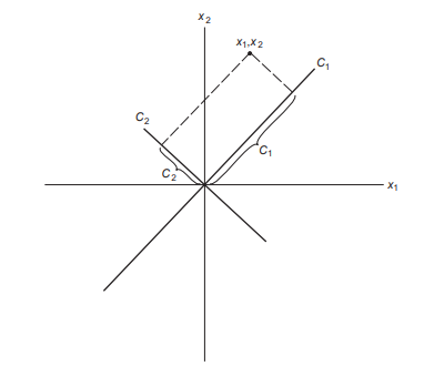
The basic idea is to create two new variables, $C_{1}$ and $C_{2}$, called the principal components. These new variables are linear functions of $x_{1}$ and $x_{2}$ and can therefore be written as
$$
\begin{aligned}
&C_{1}=a_{11} x_{1}+a_{12} x_{2} \
&C_{2}=a_{21} x_{1}+a_{22} x_{2}
\end{aligned}
$$
We note that for any set of values of the coefficients $a_{11}, a_{12}, a_{21}, a_{22}$, we can introduce the $N$ observed $x_{1}$ and $x_{2}$ and obtain $N$ values of $C_{1}$ and $C_{2}$. The means and variances of the $N$ values of $C_{1}$ and $C_{2}$ are
$$
\begin{aligned}
\text { mean } C_{1} &=\text { mean } C_{2}=0 \
\operatorname{Var} C_{1} &=a_{11}^{2} S_{1}^{2}+a_{12}^{2} S_{2}^{2}+2 a_{11} a_{12} r S_{1} S_{2} \
\operatorname{Var} C_{2} &=a_{21}^{2} S_{1}^{2}+a_{22}^{2} S_{2}^{2}+2 a_{21} a_{22} r S_{1} S_{2}
\end{aligned}
$$
where $S_{i}^{2}=\operatorname{Var} X_{i}$
统计代写|多元统计分析作业代写Multivariate Statistical Analysis代考|Interpretation
Transforming coefficients to correlations
To interpret the meaning of the first principal component, we recall that it was expressed as
$$
C_{1}=0.851 x_{1}+0.525 x_{2}
$$
The coefficient $0.851$ can be transformed into a correlation between $x_{1}$ and $C_{1}$. In general, the correlation between the $i$ th principal component and the $j$ th $x$ variable is
$$
r_{i j}=\frac{a_{i j}\left(\operatorname{Var} C_{i}\right)^{1 / 2}}{\left(\operatorname{Var} x_{j}\right)^{1 / 2}}
$$
where $a_{i j}$ is the coefficient of $x_{j}$ for the ith principal component. For example, the correlation between $C_{1}$ and $x_{1}$ is
$$
r_{11}=\frac{0.85(135.04)^{1 / 2}}{(103.98)^{1 / 2}}=0.969
$$
and the correlation between $C_{1}$ and $x_{2}$ is
$$
r_{12}=\frac{0.525(135.04)^{1 / 2}}{(53.51)^{1 / 2}}=0.834
$$
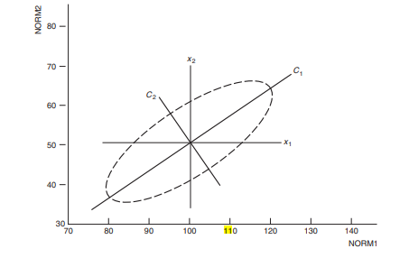
Note that both of these correlations are fairly high and positive. As can be seen from Figure 14.3, when either $x_{1}$ or $x_{2}$ increases, so will $C_{1}$. This result occurs often in principal components analysis whereby the first component is positively correlated with all of the original variables.
假设检验代写
统计代写|多元统计分析作业代写Multivariate Statistical Analysis代考|When is principal components analysis used?
进行主成分分析是为了简化一组相互关联的变量的描述。在主成分分析中,变量被平等对待;即,它们不像回归分析那样分为因变量和自变量。
该技术可以概括为一种将原始变量转换为新的、不相关的变量的方法。新变量称为主成分。每个主成分都是原始变量的线性组合。每个主成分传达的信息量的一个衡量标准是它的方差。因此,主成分按方差递减的顺序排列。因此,信息最多的主成分是第一个,而信息最少的是最后一个(方差为零的变量不区分总体成员)。
调查人员可能希望减少问题的维数,即减少变量的数量而不丢失很多信息。这个目标可以通过选择只分析前几个主成分来实现。未分析的主成分仅传达少量信息,因为它们的方差很小。这种技术之所以有吸引力是因为另一个原因,即主成分不相关。因此,调查者可以分析少量不相关的主成分,而不是分析大量具有复杂相互关系的原始变量。
选定的主成分也可用于检验它们的正态性。如果主成分不是正态分布的,那么原始变量也不是。主成分的另一个用途是搜索异常值。每个主成分的直方图可以识别具有非常大或非常小的值的个体;这些值是异常值或错误的候选值。
在回归分析中,有时获得对应于X变量,然后对选定的组件执行回归。这种策略对于克服多重共线性问题很有用,因为主成分是不相关的(Chatterjee 和 Hadi,2012 年)。主成分分析也可以看作是因子分析的一个步骤(第 15 章)。
统计代写|多元统计分析作业代写Multivariate Statistical Analysis代考|Data example
假设我们有一个随机样本ñ意见X1和X2. 为了便于解释,我们从每个观察中减去样本均值,从而获得
X1=X1−X¯1和X2=X2−X2
请注意,这种技术使X1和X2等于零但不改变样本方差小号12和小号22或相关性r.
基本思想是创建两个新变量,C1和C2,称为主成分。这些新变量是X1和X2因此可以写成
C1=一种11X1+一种12X2 C2=一种21X1+一种22X2
我们注意到,对于任何一组系数值一种11,一种12,一种21,一种22,我们可以引入ñ观察到的X1和X2并获得ñ的值C1和C2. 均值和方差ñ的值C1和C2是
意思是 C1= 意思是 C2=0 在哪里C1=一种112小号12+一种122小号22+2一种11一种12r小号1小号2 在哪里C2=一种212小号12+一种222小号22+2一种21一种22r小号1小号2
在哪里小号一世2=在哪里X一世
统计代写|多元统计分析作业代写Multivariate Statistical Analysis代考|Interpretation
将系数转换为相关性
为了解释第一个主成分的含义,我们记得它被表示为
C1=0.851X1+0.525X2
系数0.851可以转化为相关性X1和C1. 一般来说,两者之间的相关性一世主成分和jthX变量是
r一世j=一种一世j(在哪里C一世)1/2(在哪里Xj)1/2
在哪里一种一世j是系数Xj为第 i 个主成分。例如,之间的相关性C1和X1是
r11=0.85(135.04)1/2(103.98)1/2=0.969
以及之间的相关性C1和X2是
r12=0.525(135.04)1/2(53.51)1/2=0.834
请注意,这两种相关性都相当高且为正。从图 14.3 可以看出,当X1要么X2增加,所以会C1. 这个结果经常出现在主成分分析中,其中第一个成分与所有原始变量正相关。

统计代写请认准statistics-lab™. statistics-lab™为您的留学生涯保驾护航。
随机过程代考
在概率论概念中,随机过程是随机变量的集合。 若一随机系统的样本点是随机函数,则称此函数为样本函数,这一随机系统全部样本函数的集合是一个随机过程。 实际应用中,样本函数的一般定义在时间域或者空间域。 随机过程的实例如股票和汇率的波动、语音信号、视频信号、体温的变化,随机运动如布朗运动、随机徘徊等等。
贝叶斯方法代考
贝叶斯统计概念及数据分析表示使用概率陈述回答有关未知参数的研究问题以及统计范式。后验分布包括关于参数的先验分布,和基于观测数据提供关于参数的信息似然模型。根据选择的先验分布和似然模型,后验分布可以解析或近似,例如,马尔科夫链蒙特卡罗 (MCMC) 方法之一。贝叶斯统计概念及数据分析使用后验分布来形成模型参数的各种摘要,包括点估计,如后验平均值、中位数、百分位数和称为可信区间的区间估计。此外,所有关于模型参数的统计检验都可以表示为基于估计后验分布的概率报表。
广义线性模型代考
广义线性模型(GLM)归属统计学领域,是一种应用灵活的线性回归模型。该模型允许因变量的偏差分布有除了正态分布之外的其它分布。
statistics-lab作为专业的留学生服务机构,多年来已为美国、英国、加拿大、澳洲等留学热门地的学生提供专业的学术服务,包括但不限于Essay代写,Assignment代写,Dissertation代写,Report代写,小组作业代写,Proposal代写,Paper代写,Presentation代写,计算机作业代写,论文修改和润色,网课代做,exam代考等等。写作范围涵盖高中,本科,研究生等海外留学全阶段,辐射金融,经济学,会计学,审计学,管理学等全球99%专业科目。写作团队既有专业英语母语作者,也有海外名校硕博留学生,每位写作老师都拥有过硬的语言能力,专业的学科背景和学术写作经验。我们承诺100%原创,100%专业,100%准时,100%满意。
机器学习代写
随着AI的大潮到来,Machine Learning逐渐成为一个新的学习热点。同时与传统CS相比,Machine Learning在其他领域也有着广泛的应用,因此这门学科成为不仅折磨CS专业同学的“小恶魔”,也是折磨生物、化学、统计等其他学科留学生的“大魔王”。学习Machine learning的一大绊脚石在于使用语言众多,跨学科范围广,所以学习起来尤其困难。但是不管你在学习Machine Learning时遇到任何难题,StudyGate专业导师团队都能为你轻松解决。
多元统计分析代考
基础数据: $N$ 个样本, $P$ 个变量数的单样本,组成的横列的数据表
变量定性: 分类和顺序;变量定量:数值
数学公式的角度分为: 因变量与自变量
时间序列分析代写
随机过程,是依赖于参数的一组随机变量的全体,参数通常是时间。 随机变量是随机现象的数量表现,其时间序列是一组按照时间发生先后顺序进行排列的数据点序列。通常一组时间序列的时间间隔为一恒定值(如1秒,5分钟,12小时,7天,1年),因此时间序列可以作为离散时间数据进行分析处理。研究时间序列数据的意义在于现实中,往往需要研究某个事物其随时间发展变化的规律。这就需要通过研究该事物过去发展的历史记录,以得到其自身发展的规律。
回归分析代写
多元回归分析渐进(Multiple Regression Analysis Asymptotics)属于计量经济学领域,主要是一种数学上的统计分析方法,可以分析复杂情况下各影响因素的数学关系,在自然科学、社会和经济学等多个领域内应用广泛。
MATLAB代写
MATLAB 是一种用于技术计算的高性能语言。它将计算、可视化和编程集成在一个易于使用的环境中,其中问题和解决方案以熟悉的数学符号表示。典型用途包括:数学和计算算法开发建模、仿真和原型制作数据分析、探索和可视化科学和工程图形应用程序开发,包括图形用户界面构建MATLAB 是一个交互式系统,其基本数据元素是一个不需要维度的数组。这使您可以解决许多技术计算问题,尤其是那些具有矩阵和向量公式的问题,而只需用 C 或 Fortran 等标量非交互式语言编写程序所需的时间的一小部分。MATLAB 名称代表矩阵实验室。MATLAB 最初的编写目的是提供对由 LINPACK 和 EISPACK 项目开发的矩阵软件的轻松访问,这两个项目共同代表了矩阵计算软件的最新技术。MATLAB 经过多年的发展,得到了许多用户的投入。在大学环境中,它是数学、工程和科学入门和高级课程的标准教学工具。在工业领域,MATLAB 是高效研究、开发和分析的首选工具。MATLAB 具有一系列称为工具箱的特定于应用程序的解决方案。对于大多数 MATLAB 用户来说非常重要,工具箱允许您学习和应用专业技术。工具箱是 MATLAB 函数(M 文件)的综合集合,可扩展 MATLAB 环境以解决特定类别的问题。可用工具箱的领域包括信号处理、控制系统、神经网络、模糊逻辑、小波、仿真等。