如果你也在 怎样代写统计推断Statistical inference这个学科遇到相关的难题,请随时右上角联系我们的24/7代写客服。
统计推断是指从数据中得出关于种群或科学真理的结论的过程。进行推断的模式有很多,包括统计建模、面向数据的策略以及在分析中明确使用设计和随机化。
statistics-lab™ 为您的留学生涯保驾护航 在代写统计推断Statistical inference方面已经树立了自己的口碑, 保证靠谱, 高质且原创的统计Statistics代写服务。我们的专家在代写统计推断Statistical inference代写方面经验极为丰富,各种代写统计推断Statistical inference相关的作业也就用不着说。
我们提供的统计推断Statistical inference及其相关学科的代写,服务范围广, 其中包括但不限于:
- Statistical Inference 统计推断
- Statistical Computing 统计计算
- Advanced Probability Theory 高等概率论
- Advanced Mathematical Statistics 高等数理统计学
- (Generalized) Linear Models 广义线性模型
- Statistical Machine Learning 统计机器学习
- Longitudinal Data Analysis 纵向数据分析
- Foundations of Data Science 数据科学基础
统计代写|统计推断代写Statistical inference代考|Cumulant-generating functions and cumulants
It is often convenient to work with the log of the moment-generating function. It turns out that the coefficients of the polynomial expansion of the log of the momentgenerating function have convenient interpretations in terms of moments and central moments.
Definition 3.5.7 (Cumulant-generating function and cumulants)
The cumulant-generating function of a random variable $X$ with moment-generating function $M_{X}(t)$, is defined as
$$
K_{X}(t)=\log M_{X}(t)
$$
The $r^{\text {th }}$ cumulant, $K_{r}$, is the coefficient of $t^{r} / r !$ in the expansion of the cumulantgenerating function $K_{X}(t)$ so
$$
K_{X}(t)=\kappa_{1} t+\kappa_{2} \frac{t^{2}}{2 !}+\ldots+\kappa_{r} \frac{t^{r}}{r !}+\ldots=\sum_{j=1}^{\infty} K_{j} \frac{t^{j}}{j !}
$$
It is clear from this definition that the relationship between cumulant-generating function and cumulants is the same as the relationship between moment-generating function and moments. Thus, to calculate cumulants we can either compare coefficients or differentiate.
- Calculating the $r^{\text {th }}$ cumulant, $\kappa_{r}$, by comparing coefficients:
$$
\text { if } K_{X}(t)=\sum_{j=0}^{\infty} b_{j} t^{j} \text { then } K_{r}=r ! b_{r} \text {. }
$$ - Calculating the $r^{\text {th }}$ cumulant, $\kappa_{r}$, by differentiation:
$$
K_{r}=K_{X}^{(r)}(0)=\left.\frac{d^{r}}{d t^{r}} K_{X}(t)\right|_{t=0}
$$
Cumulants can be expressed in terms of moments and central moments. Particularly useful are the facts that the first cumulant is the mean and the second cumulant is the variance. In order to prove these results we will use the expansion, for $|x|<1$,
$$
\log (1+x)=x-\frac{1}{2} x^{2}+\frac{1}{3} x^{3}-\ldots+\frac{(-1)^{j+1}}{j} x^{j}+\ldots
$$
统计代写|统计推断代写Statistical inference代考|Distribution and mass/density for g(X)
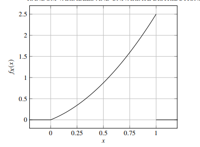
Suppose that $X$ is a random variable defined on $(\Omega, \mathcal{F}, \mathrm{P})$ and $g: \mathbb{R} \rightarrow \mathbb{R}$ is a well-behaved function. We would like to derive an expression for the cumulative distribution function of $Y$, where $Y=g(X)$. Some care is required here. We define $g$ to be a function, so for every real number input there is a single real number output. However, $g^{-1}$ is not necessarily a function, so a single input may have multiple outputs. To illustrate, let $g(x)=x^{2}$, then $g^{-1}$ corresponds to taking the square root, an operation that typically has two real outputs; for example, $g^{-1}(4)={-2,2}$. So, in general,
$$
\mathrm{P}(Y \leq y)=\mathrm{P}(g(X) \leq y) \neq \mathrm{P}\left(X \leq g^{-1}(y)\right)
$$
Our first step in deriving an expression for the distribution function of $Y$ is to consider the probability that $Y$ takes values in a subset of $\mathbb{R}$. We will use the idea of the inverse image of a set.
Definition 3.6.1 (Inverse image)
If $g: R \rightarrow R$ is a function and $B$ is a subset of real numbers, then the inverse image of $B$ under $g$ is the set of real numbers whose images under $g$ lie in $B$, that is, for all $B \subseteq \mathbb{R}$ we define the inverse image of $B$ under $g$ as
$$
g^{-1}(B)={x \in \mathbb{R}: g(x) \in B}
$$
Then for any well-behaved $B \subseteq \mathbb{R}$,
$$
\begin{aligned}
\mathrm{P}(Y \in B) &=\mathrm{P}(g(X) \in B)=\mathrm{P}({\omega \in \Omega: g(X(\omega)) \in B}) \
&=\mathrm{P}\left(\left{\omega \in \Omega: X(\omega) \in g^{-1}(B)\right}\right)=\mathrm{P}\left(X \in g^{-1}(B)\right)
\end{aligned}
$$
Stated loosely, the probability that $g(X)$ is in $B$ is equal to the probability that $X$ is in the inverse image of $B$. The cumulative distribution function of $Y$ is then
$$
\begin{aligned}
F_{Y}(y) &=\mathrm{P}(Y \leq y)=\mathrm{P}(Y \in(-\infty, y])=\mathrm{P}(g(X) \in(-\infty, y]) \
&=\mathrm{P}\left(X \in g^{-1}((-\infty, y])\right) \
&= \begin{cases}\sum_{{x: g(x) \leq y}} f_{X}(x) & \text { if } X \text { is discrete, } \
\int_{{x: g(x) \leq y}} f_{X}(x) d x & \text { if } X \text { is continuous. }\end{cases}
\end{aligned}
$$
In the discrete case, we can use similar reasoning to provide an expression for the mass function,
$$
f_{Y}(y)=\mathrm{P}(Y=y)=\mathrm{P}(g(X)=y)=\mathrm{P}\left(X \in g^{-1}(y)\right)=\sum_{{x: g(x)=y}} f_{X}(x)
$$
统计代写|统计推断代写Statistical inference代考|Sequences of random variables and convergence
Suppose that $x_{1}, x_{2}, \ldots$ is a sequence of real numbers. We denote this sequence $\left{x_{n}\right}$. The definition of convergence for a sequence of real numbers is well established.
Definition 3.7.1 (Convergence of a real sequence)
Let $\left{x_{n}\right}$ be a sequence of real numbers and let $x$ be a real number. We say that $x_{n}$ converges to $x$ if and only if, for every $\varepsilon>0$, we can find an integer $N$ such that $\left|x_{n}-x\right|<\varepsilon$ for all $n>N$. Under these conditions, we write $x_{n} \rightarrow x$ as $n \rightarrow \infty$.
This definition is based on an intuitively appealing idea (although in the formal statement given above, this might not be obvious). If we take any interval around $x$, say $[x-\varepsilon, x+\varepsilon]$, we can find a point, say $N$, beyond which all elements of the sequence fall in the interval. This is true for an arbitrarily small interval.
Now consider a sequence of random variables $\left{X_{n}\right}$ and a random variable $X$. We want to know what it means for $\left{X_{n}\right}$ to converge to $X$. Using Definition 3.7.1 is not possible; since $\left|X_{n}-X\right|$ is a random variable, direct comparison with the real number $\varepsilon$ is not meaningful. In fact, for a random variable there are many different forms of convergence. We define four distinct modes of convergence for a sequence of random variables.
统计推断代考
统计代写|统计推断代写Statistical inference代考|Cumulant-generating functions and cumulants
使用矩生成函数的日志通常很方便。事实证明,矩生成函数的对数的多项式展开系数在矩和中心矩方面具有方便的解释。
定义 3.5.7(累积量生成函数和累积量)
随机变量的累积量生成函数X具有力矩生成功能米X(吨), 定义为
ķX(吨)=日志米X(吨)
这rth 累积,ķr,是系数吨r/r!在累积量生成函数的扩展中ķX(吨)所以
ķX(吨)=ķ1吨+ķ2吨22!+…+ķr吨rr!+…=∑j=1∞ķj吨jj!
从这个定义可以清楚地看出,累积量生成函数和累积量之间的关系与矩生成函数和矩之间的关系是一样的。因此,要计算累积量,我们可以比较系数或微分。
- 计算rth 累积,ķr,通过比较系数:
如果 ķX(吨)=∑j=0∞bj吨j 然后 ķr=r!br. - 计算rth 累积,ķr,通过微分:
ķr=ķX(r)(0)=drd吨rķX(吨)|吨=0
累积量可以用矩和中心矩来表示。特别有用的是第一个累积量是平均值,第二个累积量是方差。为了证明这些结果,我们将使用展开式,对于|X|<1,
日志(1+X)=X−12X2+13X3−…+(−1)j+1jXj+…
统计代写|统计推断代写Statistical inference代考|Distribution and mass/density for g(X)
假设X是一个随机变量,定义在(Ω,F,磷)和G:R→R是一个表现良好的函数。我们想推导出累积分布函数的表达式是, 在哪里是=G(X). 这里需要一些小心。我们定义G成为一个函数,因此对于每个实数输入,都有一个实数输出。然而,G−1不一定是函数,因此单个输入可能有多个输出。为了说明,让G(X)=X2, 然后G−1对应于取平方根,这种操作通常有两个实数输出;例如,G−1(4)=−2,2. 所以,一般来说,
磷(是≤是)=磷(G(X)≤是)≠磷(X≤G−1(是))
我们的第一步是导出分布函数的表达式是是考虑概率是取值的子集R. 我们将使用集合的逆像的概念。
定义 3.6.1(反图像)
如果G:R→R是一个函数并且乙是实数的子集,则乙在下面G是一组实数,其图像在G位于乙,也就是说,对于所有乙⊆R我们定义的逆像乙在下面G作为
G−1(乙)=X∈R:G(X)∈乙
那么对于任何表现良好的乙⊆R,
\begin{对齐} \mathrm{P}(Y\inB) &=\mathrm{P}(g(X)\inB)=\mathrm{P}({\omega\in\Omega: g(X (\ omega))\in B})\&=\mathrm{P}\left(\left{\omega\in\Omega:X(\omega)\in g^{-1}(B)\right} \right )=\mathrm{P}\left(X\in g^{-1}(B)\right)\end{aligned}\begin{对齐} \mathrm{P}(Y\inB) &=\mathrm{P}(g(X)\inB)=\mathrm{P}({\omega\in\Omega: g(X (\ omega))\in B})\&=\mathrm{P}\left(\left{\omega\in\Omega:X(\omega)\in g^{-1}(B)\right} \right )=\mathrm{P}\left(X\in g^{-1}(B)\right)\end{aligned}
松散地说,概率G(X)在乙等于概率X是在相反的图像乙. 的累积分布函数是那么是
F是(是)=磷(是≤是)=磷(是∈(−∞,是])=磷(G(X)∈(−∞,是]) =磷(X∈G−1((−∞,是])) ={∑X:G(X)≤是FX(X) 如果 X 是离散的, ∫X:G(X)≤是FX(X)dX 如果 X 是连续的。
在离散情况下,我们可以使用类似的推理来提供质量函数的表达式,
F是(是)=磷(是=是)=磷(G(X)=是)=磷(X∈G−1(是))=∑X:G(X)=是FX(X)
统计代写|统计推断代写Statistical inference代考|Sequences of random variables and convergence
假设X1,X2,…是实数序列。我们表示这个序列\左{x_{n}\右}\左{x_{n}\右}. 实数序列收敛性的定义已经确立。
定义 3.7.1(实数列的收敛)
令\左{x_{n}\右}\左{x_{n}\右}是一个实数序列,让X是一个实数。我们说Xn收敛到X当且仅当,对于每个e>0,我们可以找到一个整数ñ这样|Xn−X|<e对所有人n>ñ. 在这些条件下,我们写Xn→X作为n→∞.
这个定义基于一个直观吸引人的想法(尽管在上面给出的正式声明中,这可能并不明显)。如果我们采取任何间隔X, 说[X−e,X+e],我们可以找到一个点,比如说ñ, 超出该序列的所有元素都落在区间内。对于任意小的间隔都是如此。
现在考虑一系列随机变量\left{X_{n}\right}\left{X_{n}\right}和一个随机变量X. 我们想知道这意味着什么\left{X_{n}\right}\left{X_{n}\right}收敛到X. 使用定义 3.7.1 是不可能的;自从|Xn−X|是随机变量,直接与实数比较e没有意义。事实上,对于一个随机变量,有许多不同形式的收敛。我们为一系列随机变量定义了四种不同的收敛模式。

统计代写请认准statistics-lab™. statistics-lab™为您的留学生涯保驾护航。
金融工程代写
金融工程是使用数学技术来解决金融问题。金融工程使用计算机科学、统计学、经济学和应用数学领域的工具和知识来解决当前的金融问题,以及设计新的和创新的金融产品。
非参数统计代写
非参数统计指的是一种统计方法,其中不假设数据来自于由少数参数决定的规定模型;这种模型的例子包括正态分布模型和线性回归模型。
广义线性模型代考
广义线性模型(GLM)归属统计学领域,是一种应用灵活的线性回归模型。该模型允许因变量的偏差分布有除了正态分布之外的其它分布。
术语 广义线性模型(GLM)通常是指给定连续和/或分类预测因素的连续响应变量的常规线性回归模型。它包括多元线性回归,以及方差分析和方差分析(仅含固定效应)。
有限元方法代写
有限元方法(FEM)是一种流行的方法,用于数值解决工程和数学建模中出现的微分方程。典型的问题领域包括结构分析、传热、流体流动、质量运输和电磁势等传统领域。
有限元是一种通用的数值方法,用于解决两个或三个空间变量的偏微分方程(即一些边界值问题)。为了解决一个问题,有限元将一个大系统细分为更小、更简单的部分,称为有限元。这是通过在空间维度上的特定空间离散化来实现的,它是通过构建对象的网格来实现的:用于求解的数值域,它有有限数量的点。边界值问题的有限元方法表述最终导致一个代数方程组。该方法在域上对未知函数进行逼近。[1] 然后将模拟这些有限元的简单方程组合成一个更大的方程系统,以模拟整个问题。然后,有限元通过变化微积分使相关的误差函数最小化来逼近一个解决方案。
tatistics-lab作为专业的留学生服务机构,多年来已为美国、英国、加拿大、澳洲等留学热门地的学生提供专业的学术服务,包括但不限于Essay代写,Assignment代写,Dissertation代写,Report代写,小组作业代写,Proposal代写,Paper代写,Presentation代写,计算机作业代写,论文修改和润色,网课代做,exam代考等等。写作范围涵盖高中,本科,研究生等海外留学全阶段,辐射金融,经济学,会计学,审计学,管理学等全球99%专业科目。写作团队既有专业英语母语作者,也有海外名校硕博留学生,每位写作老师都拥有过硬的语言能力,专业的学科背景和学术写作经验。我们承诺100%原创,100%专业,100%准时,100%满意。
随机分析代写
随机微积分是数学的一个分支,对随机过程进行操作。它允许为随机过程的积分定义一个关于随机过程的一致的积分理论。这个领域是由日本数学家伊藤清在第二次世界大战期间创建并开始的。
时间序列分析代写
随机过程,是依赖于参数的一组随机变量的全体,参数通常是时间。 随机变量是随机现象的数量表现,其时间序列是一组按照时间发生先后顺序进行排列的数据点序列。通常一组时间序列的时间间隔为一恒定值(如1秒,5分钟,12小时,7天,1年),因此时间序列可以作为离散时间数据进行分析处理。研究时间序列数据的意义在于现实中,往往需要研究某个事物其随时间发展变化的规律。这就需要通过研究该事物过去发展的历史记录,以得到其自身发展的规律。
回归分析代写
多元回归分析渐进(Multiple Regression Analysis Asymptotics)属于计量经济学领域,主要是一种数学上的统计分析方法,可以分析复杂情况下各影响因素的数学关系,在自然科学、社会和经济学等多个领域内应用广泛。
MATLAB代写
MATLAB 是一种用于技术计算的高性能语言。它将计算、可视化和编程集成在一个易于使用的环境中,其中问题和解决方案以熟悉的数学符号表示。典型用途包括:数学和计算算法开发建模、仿真和原型制作数据分析、探索和可视化科学和工程图形应用程序开发,包括图形用户界面构建MATLAB 是一个交互式系统,其基本数据元素是一个不需要维度的数组。这使您可以解决许多技术计算问题,尤其是那些具有矩阵和向量公式的问题,而只需用 C 或 Fortran 等标量非交互式语言编写程序所需的时间的一小部分。MATLAB 名称代表矩阵实验室。MATLAB 最初的编写目的是提供对由 LINPACK 和 EISPACK 项目开发的矩阵软件的轻松访问,这两个项目共同代表了矩阵计算软件的最新技术。MATLAB 经过多年的发展,得到了许多用户的投入。在大学环境中,它是数学、工程和科学入门和高级课程的标准教学工具。在工业领域,MATLAB 是高效研究、开发和分析的首选工具。MATLAB 具有一系列称为工具箱的特定于应用程序的解决方案。对于大多数 MATLAB 用户来说非常重要,工具箱允许您学习和应用专业技术。工具箱是 MATLAB 函数(M 文件)的综合集合,可扩展 MATLAB 环境以解决特定类别的问题。可用工具箱的领域包括信号处理、控制系统、神经网络、模糊逻辑、小波、仿真等。