如果你也在 怎样代写非参数统计Nonparametric Statistics这个学科遇到相关的难题,请随时右上角联系我们的24/7代写客服。
非参数统计Nonparametric Statistics指的是一种统计方法,其中不假设数据来自于由少数参数决定的规定模型;这种模型的例子包括正态分布模型和线性回归模型。
statistics-lab™ 为您的留学生涯保驾护航 在代写非参数统计Nonparametric Statistics方面已经树立了自己的口碑, 保证靠谱, 高质且原创的统计Statistics代写服务。我们的专家在代写非参数统计Nonparametric Statistics代写方面经验极为丰富,各种代写非参数统计Nonparametric Statistics相关的作业也就用不着 说。
我们提供的多元非参数统计Nonparametric Statistics及其相关学科的代写,服务范围广, 其中包括但不限于:
- Statistical Inference 统计推断
- Statistical Computing 统计计算
- Advanced Probability Theory 高等楖率论
- Advanced Mathematical Statistics 高等数理统计学
- (Generalized) Linear Models 广义线性模型
- Statistical Machine Learning 统计机器学习
- Longitudinal Data Analysis 纵向数据 分析
- Foundations of Data Science 数据科学基础

统计代写|非参数统计代写Nonparametric Statistics代考|Two-Sample Estimation and Confidence Intervals
Denote the samples as $X_{1}, \ldots, X_{M_{1}}$ and $Y_{1}, \ldots, Y_{M_{2}}$ as before. Let $\theta$ represent the amount by which a location parameter for the population from which the second sample exceeds that of the first sample. Under the assumption (3.1) that the distributions are identical up to shift, then
$$
X_{1}, \ldots, X_{M_{1}}, Y_{1}-\theta, \ldots, Y_{M_{2}}-\theta
$$
all have the same distribution. Then let $T_{G}^{{2}}(\theta)$ be the general rank statistic (3.7) calculated from this data set (3.29).
Most commonly the scores are chosen to make $T_{G}^{{2}}(\theta)$ the Wilcoxon ranksum statistic, or equivalently the Mann-Whitney statistic, but conceptually this could be done by inverting, for example, Mood’s median test or any other rank test. For general scores $a_{j}, T_{G}^{{2}}(\theta)=\sum_{j=1}^{N} a_{j} Z_{j}(\theta)$, where $Z_{j}(\theta)$ is 1 if item ranked $j$ among (3.29) came from $Y$, and 0 otherwise.
One can define an estimator as that value of $\theta$ that makes this test statistic equal to its null expectation; that is, $\hat{\theta}$ solves
$$
T_{G}^{{2}}(\hat{\theta})=M_{2} \bar{a} .
$$
Furthermore, one can determine the largest integer $t_{l}$ and smallest integer $t_{u}$ such that
$$
\mathrm{P}{0}\left[T{G}^{{2}}(0)<t_{l}\right] \leq \alpha / 2, \quad \mathrm{P}{0}\left[T{G}^{{2}}(0) \geq t_{u}\right] \leq \alpha / 2
$$
in close parallel with definitions of $\S 2.3 .2$. Then, reject the null hypothesis if $T_{G}^{{2}}\left(\theta^{\circ}\right) \leq t_{L}^{\circ}$ or $T_{G}^{{2}}\left(\theta^{\circ}\right) \geq t_{U}^{\circ}$ for $t_{L}^{\circ}=t_{l}-1$ and $t_{U}^{\circ}=t_{u}$, and use as the confidence interval
$$
\left{\theta \mid t_{l} \leq T_{G}^{{2}}\left(\theta^{0}\right)<t_{u}\right}
$$
Applying the Gaussian approximation to $T_{G}^{{2}}(\theta)$,
$$
t_{l}, t_{u} \approx M_{2} \bar{a} \pm z_{\alpha / 2} \sqrt{\operatorname{Var}\left[T_{G}^{{2}}(0)\right]}
$$
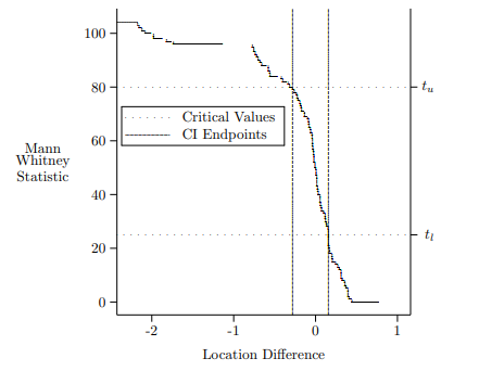
统计代写|非参数统计代写Nonparametric Statistics代考|Inversion of the Mann-Whitney-Wilcoxon Test
When $a_{j}$ are ranks $j, T_{G}^{{2}}(\theta)$ is the Wilcoxon version of the test. The corresponding Mann-Whitney version $T_{U}(\theta)=\sum_{i} \sum_{j} I\left(X_{i}\theta\right)
$$
is $\left{\theta \mid t_{l} \leq T_{U}^{{2}}(\theta)<t_{u}\right}$, for the largest $t_{l}$ and smallest $t_{u}$ as in (3.31), made specific to the Mann-Whitney statistic:
$$
\sum_{k=0}^{t_{1}-1} \mathrm{P}{M{1}, M_{2}}\left[T_{U}^{{2}}(0)=k\right] \leq \frac{\alpha}{2}, \sum_{k=t_{u}}^{M_{1} M_{2}} \mathrm{P}{M{1}, M_{2}}\left[T_{U}^{{2}}(0)=k\right] \leq \frac{\alpha}{2},
$$
统计代写|非参数统计代写Nonparametric Statistics代考|Tests for Broad Alternatives
Use the empirical cumulative distribution function estimator as in $\S 2.5$. The Kolmogorov-Smirnov test uses the largest difference between these as the test statistic. The null hypothesis under the permutation distribution is formed from all permutations of data between the two samples. The $p$-value is the portion with as large or larger difference. If the number of such permutations is quite large, one might use a random sample instead. Asymptotic approximations to these distributions exist as well. Calculation of these statistics can be simplified by noting that the maximum may be calculated from differences in the empirical cumulative distribution functions evaluated exclusively at jumps in one or the other curve.
Alternatively, one might use the integral of difference between these, squared, as the test statistic; this statistic is called the Cramér-von Mises test. That is, if $\hat{F}$ and $\hat{G}$ are the empirical distribution functions for the two samples, then the test statistic is $\int_{-\infty}^{\infty}|\hat{F}-\hat{G}|^{2}\left(M_{1} d \hat{F}+M_{2} d \hat{G}\right) / N$; this integral is in the sense of Stieltjes $(1894)$, and is calculated as the average over all values in the combined sample of the difference between empirical distributions, squared. Conceptually, to implement this test, use all permutations of data between the two samples, and count the proportion with as large or
多元统计分析代写
统计代写|非参数统计代写Nonparametric Statistics代考|Two-Sample Estimation and Confidence Intervals
将样本表示为X1,…,X米1和和1,…,和米2像之前一样。让θ表示第二个样本的总体位置参数超过第一个样本的位置参数的数量。在假设(3.1)的分布是相同的转移,然后
X1,…,X米1,和1−θ,…,和米2−θ
都具有相同的分布。然后让吨G2(θ)是从该数据集 (3.29) 计算的一般等级统计量 (3.7)。
最常见的分数被选择为吨G2(θ)Wilcoxon ranksum 统计量,或等效的 Mann-Whitney 统计量,但从概念上讲,这可以通过反转例如 Mood 中位数检验或任何其他等级检验来完成。一般分数一种j,吨G2(θ)=∑j=1ñ一种j和j(θ), 在哪里和j(θ)如果项目排名为 1j其中 (3.29) 来自和, 否则为 0。
可以将估计量定义为θ使该检验统计量等于其零期望;那是,θ^解决
吨G2(θ^)=米2一种¯.
此外,可以确定最大的整数吨一世和最小整数吨你使得
$$
\mathrm{P} {0}\left[T {G}^{{2}}(0)<t_{l}\right] \leq \alpha / 2, \quad \mathrm{P} {0}\left[T {G}^{{2}}(0) \geq t_{u}\right] \leq \alpha / 2
§一世nC一世○s和p一种r一种一世一世和一世在一世吨Hd和F一世n一世吨一世○ns○F$§2.3.2$.吨H和n,r和j和C吨吨H和n你一世一世H和p○吨H和s一世s一世F$吨G2(θ∘)≤吨一世∘$○r$吨G2(θ∘)≥吨ü∘$F○r$吨一世∘=吨一世−1$一种nd$吨ü∘=吨你$,一种nd你s和一种s吨H和C○nF一世d和nC和一世n吨和rv一种一世
\left{\theta \mid t_{l} \leq T_{G}^{{2}}\left(\theta^{0}\right)<t_{u}\right}
一种pp一世和一世nG吨H和G一种你ss一世一种n一种ppr○X一世米一种吨一世○n吨○$吨G2(θ)$,
t_{l}, t_{u} \approx M_{2} \bar{a} \pm z_{\alpha / 2} \sqrt{\operatorname{Var}\left[T_{G}^{{2}} (0)\right]}
$$
统计代写|非参数统计代写Nonparametric Statistics代考|Inversion of the Mann-Whitney-Wilcoxon Test
什么时候一种j是等级j,吨G2(θ)是测试的 Wilcoxon 版本。相应的曼惠特尼版本吨ü(θ)=∑一世∑j一世(X一世θ)一世s\left{\theta \mid t_{l} \leq T_{U}^{{2}}(\theta)<t_{u}\right},F○r吨H和一世一种rG和s吨t_{l}一种nds米一种一世一世和s吨t_{u}一种s一世n(3.31),米一种d和sp和C一世F一世C吨○吨H和米一种nn−在H一世吨n和和s吨一种吨一世s吨一世C:∑到=0吨1−1磷米1,米2[吨ü2(0)=到]≤一种2,∑到=吨你米1米2磷米1,米2[吨ü2(0)=到]≤一种2,$
统计代写|非参数统计代写Nonparametric Statistics代考|Tests for Broad Alternatives
使用经验累积分布函数估计器,如§§2.5. Kolmogorov-Smirnov 检验使用这些之间的最大差异作为检验统计量。排列分布下的原假设是由两个样本之间的所有数据排列形成的。这p-value 是具有相同或更大差异的部分。如果这种排列的数量很大,则可以使用随机样本。这些分布的渐近近似也存在。这些统计数据的计算可以通过注意可以根据经验累积分布函数的差异来计算来简化,这些差异仅在一条或另一条曲线的跳跃处评估。
或者,可以使用它们之间的差的积分,平方,作为检验统计量;该统计量称为 Cramer-von Mises 检验。也就是说,如果F^和G^是两个样本的经验分布函数,则检验统计量为∫−∞∞|F^−G^|2(米1dF^+米2dG^)/ñ; 这个积分在 Stieltjes 的意义上(1894),并且计算为经验分布之间差异的组合样本中所有值的平均值,平方。从概念上讲,要实现此测试,请使用两个样本之间数据的所有排列,并计算与

统计代写请认准statistics-lab™. statistics-lab™为您的留学生涯保驾护航。
随机过程代考
在概率论概念中,随机过程是随机变量的集合。 若一随机系统的样本点是随机函数,则称此函数为样本函数,这一随机系统全部样本函数的集合是一个随机过程。 实际应用中,样本函数的一般定义在时间域或者空间域。 随机过程的实例如股票和汇率的波动、语音信号、视频信号、体温的变化,随机运动如布朗运动、随机徘徊等等。
贝叶斯方法代考
贝叶斯统计概念及数据分析表示使用概率陈述回答有关未知参数的研究问题以及统计范式。后验分布包括关于参数的先验分布,和基于观测数据提供关于参数的信息似然模型。根据选择的先验分布和似然模型,后验分布可以解析或近似,例如,马尔科夫链蒙特卡罗 (MCMC) 方法之一。贝叶斯统计概念及数据分析使用后验分布来形成模型参数的各种摘要,包括点估计,如后验平均值、中位数、百分位数和称为可信区间的区间估计。此外,所有关于模型参数的统计检验都可以表示为基于估计后验分布的概率报表。
广义线性模型代考
广义线性模型(GLM)归属统计学领域,是一种应用灵活的线性回归模型。该模型允许因变量的偏差分布有除了正态分布之外的其它分布。
statistics-lab作为专业的留学生服务机构,多年来已为美国、英国、加拿大、澳洲等留学热门地的学生提供专业的学术服务,包括但不限于Essay代写,Assignment代写,Dissertation代写,Report代写,小组作业代写,Proposal代写,Paper代写,Presentation代写,计算机作业代写,论文修改和润色,网课代做,exam代考等等。写作范围涵盖高中,本科,研究生等海外留学全阶段,辐射金融,经济学,会计学,审计学,管理学等全球99%专业科目。写作团队既有专业英语母语作者,也有海外名校硕博留学生,每位写作老师都拥有过硬的语言能力,专业的学科背景和学术写作经验。我们承诺100%原创,100%专业,100%准时,100%满意。
机器学习代写
随着AI的大潮到来,Machine Learning逐渐成为一个新的学习热点。同时与传统CS相比,Machine Learning在其他领域也有着广泛的应用,因此这门学科成为不仅折磨CS专业同学的“小恶魔”,也是折磨生物、化学、统计等其他学科留学生的“大魔王”。学习Machine learning的一大绊脚石在于使用语言众多,跨学科范围广,所以学习起来尤其困难。但是不管你在学习Machine Learning时遇到任何难题,StudyGate专业导师团队都能为你轻松解决。
多元统计分析代考
基础数据: $N$ 个样本, $P$ 个变量数的单样本,组成的横列的数据表
变量定性: 分类和顺序;变量定量:数值
数学公式的角度分为: 因变量与自变量
时间序列分析代写
随机过程,是依赖于参数的一组随机变量的全体,参数通常是时间。 随机变量是随机现象的数量表现,其时间序列是一组按照时间发生先后顺序进行排列的数据点序列。通常一组时间序列的时间间隔为一恒定值(如1秒,5分钟,12小时,7天,1年),因此时间序列可以作为离散时间数据进行分析处理。研究时间序列数据的意义在于现实中,往往需要研究某个事物其随时间发展变化的规律。这就需要通过研究该事物过去发展的历史记录,以得到其自身发展的规律。
回归分析代写
多元回归分析渐进(Multiple Regression Analysis Asymptotics)属于计量经济学领域,主要是一种数学上的统计分析方法,可以分析复杂情况下各影响因素的数学关系,在自然科学、社会和经济学等多个领域内应用广泛。
MATLAB代写
MATLAB 是一种用于技术计算的高性能语言。它将计算、可视化和编程集成在一个易于使用的环境中,其中问题和解决方案以熟悉的数学符号表示。典型用途包括:数学和计算算法开发建模、仿真和原型制作数据分析、探索和可视化科学和工程图形应用程序开发,包括图形用户界面构建MATLAB 是一个交互式系统,其基本数据元素是一个不需要维度的数组。这使您可以解决许多技术计算问题,尤其是那些具有矩阵和向量公式的问题,而只需用 C 或 Fortran 等标量非交互式语言编写程序所需的时间的一小部分。MATLAB 名称代表矩阵实验室。MATLAB 最初的编写目的是提供对由 LINPACK 和 EISPACK 项目开发的矩阵软件的轻松访问,这两个项目共同代表了矩阵计算软件的最新技术。MATLAB 经过多年的发展,得到了许多用户的投入。在大学环境中,它是数学、工程和科学入门和高级课程的标准教学工具。在工业领域,MATLAB 是高效研究、开发和分析的首选工具。MATLAB 具有一系列称为工具箱的特定于应用程序的解决方案。对于大多数 MATLAB 用户来说非常重要,工具箱允许您学习和应用专业技术。工具箱是 MATLAB 函数(M 文件)的综合集合,可扩展 MATLAB 环境以解决特定类别的问题。可用工具箱的领域包括信号处理、控制系统、神经网络、模糊逻辑、小波、仿真等。