如果你也在 怎样代写广义线性模型Generalized Linear Model这个学科遇到相关的难题,请随时右上角联系我们的24/7代写客服。在統計學上,廣義線性模型(generalized linear model,缩写作GLM) 是一種應用灵活的線性迴歸模型。该模型允许因变量的偏差分布有除了正态分布之外的其它分布。
statistics-lab™ 为您的留学生涯保驾护航 在代写广义线性模型Generalized Linear Model方面已经树立了自己的口碑, 保证靠谱, 高质且原创的统计Statistics代写服务。我们的专家在代写广义线性模型Generalized Linear Model代写方面经验极为丰富,各种代写广义线性模型Generalized Linear Model相关的作业也就用不着 说。
我们提供的代写广义线性模型Generalized Linear Model及其相关学科的代写,服务范围广, 其中包括但不限于:
- 极大似然 Maximum likelihood
- 贝叶斯方法 Bayesian methods
- 线性回归 Linear regression
- 多项式Logistic回归 Multinomial regression
- 采样理论 sampling theory
统计代写| 广义线性模型project代写Generalized Linear Model代考|Latent Variables
In prospective sampling, the predictors are fixed and then the outcome is observed. This is also called a cohort study. In the infant respiratory disease example shown in Table $4.1$, we would select a sample of newborn girls and boys whose parents had chosen a particular method of feeding and then monitor them for their first year.
In retrospective sampling, the outcome is fixed and then the predictors are observed. This is also called a case-control study. Typically, we would find infants coming to a doctor with a respiratory disease in the first year and then record their sex and method of feeding. We would also obtain a sample of respiratory diseasefree infants and record their information. The method for obtaining the samples is important – we require that the probability of inclusion in the study is independent of the predictor values.
Since the question of interest is how the predictors affect the response, prospective sampling seems to be required. Let’s focus on just boys who are breast or bottle fed. The data we need is:
babyfood $[c(1,3),$,
disease nondisease sex food
$\begin{array}{lll}1 & 77 & 381 \text { Boy Bottle } \ 3 & 47 & 447 \text { Boy Breast }\end{array}$
As we have seen in Section 2.2, the log-odds is a sensible way to measure the strength of the association of a predictor with the outcome.
- Given the infant is breast fed, the log-odds of having a respiratory disease are $\log 47 / 447=-2.25$.
- Given the infant is bottle fed, the log-odds of having a respiratory disease are $\log 77 / 381=-1.60$.
The difference between these two log-odds, $\Delta=-1.60–2.25=0.65$, represents the increased risk of respiratory disease incurred by bottle feeding relative to breast feeding. This is the log-odds ratio. In this case, the log-odds ratio is positive indicating a greater risk of respiratory disease for bottle-fed compared to breast-fed babies.
Now suppose that this had been a retrospective study – we could compute the log-odds of feeding type given respiratory disease status and then find the difference.
统计代写| 广义线性模型project代写Generalized Linear Model代考|Prediction and Effective Doses
This is not a wide interval in absolute terms, but in relative terms, it certainly is. The upper limit is about 100 times larger than the lower limit.
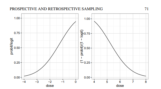
When there is a single (continuous) covariate or when other covariates are held fixed, we sometimes wish to estimate the value of $x$ corresponding to a chosen $p$. For example, we may wish to determine which dose, $x$, will lead to a probability of success $p$. ED50 stands for the effective dose for which there will be a $50 \%$ chance of success. When the objective is to kill the subjects or determine toxicity, as when using insecticides, the term LD50 would be used. LD stands for lethal dose. Other percentiles are also of interest. For a logit link, we can set $p=1 / 2$ and then solve for $x$ to find:
$$
\widehat{\mathrm{ED} 50}=-\hat{\beta}{0} / \hat{\beta}{1}
$$
Using the Bliss data, the LD50 is:
$(1 \mathrm{~d} 50<-1 \bmod \$ \operatorname{coe}[1] / 1 \bmod \$ \operatorname{coe}[2])$
(Intercept)
To determine the standard error, we can use the delta method. The general expression for the variance of $g(\hat{\theta})$ for multivariate $\theta$ is given by
$$
\operatorname{var} g(\hat{\theta}) \approx g^{\prime}(\hat{\theta})^{T} \operatorname{var} \hat{\theta} g^{\prime}(\hat{\theta})
$$
which, in this example, works out as:
$\mathrm{dr}<-c(-1 / 1 \bmod \$ c o e f[2], 1 \mathrm{mod} \$ \operatorname{coe}[11] / 1 \bmod \$ c o e f[2] \wedge 2)$
sqrt (dr of:? 1modsum\$cov. un of * क्ष $\mathrm{dr}$ ) [,]
[1] $0.17844$
So the $95 \%$ CI is given by:
$c(2-1.96 * 0.178,2+1.96 * 0.178)$
[1] $1.65112 .3489$
Other levels may be considered – the effective dose $x_{p}$ for probability of success $p$ is:
$$
x_{p}=\frac{\operatorname{logit}(p)-\beta_{0}}{\beta_{1}}
$$
假设检验代写
统计代写| 广义线性模型project代写Generalized Linear Model代考|Latent Variables
在前瞻性抽样中,预测变量是固定的,然后观察结果。这也称为队列研究。在表中所示的婴儿呼吸道疾病示例中4.1,我们将选择父母选择了特定喂养方法的新生女孩和男孩作为样本,然后对他们进行第一年的监测。
在回顾性抽样中,结果是固定的,然后观察预测变量。这也称为病例对照研究。通常,我们会发现婴儿在第一年就患有呼吸道疾病就医,然后记录他们的性别和喂养方式。我们还将获得无呼吸道疾病婴儿的样本并记录他们的信息。获取样本的方法很重要——我们要求纳入研究的概率与预测值无关。
由于感兴趣的问题是预测变量如何影响响应,因此似乎需要前瞻性抽样。让我们只关注母乳喂养或奶瓶喂养的男孩。我们需要的数据是:
婴儿食品[C(1,3),,
疾病无病性食品
177381 男孩瓶 347447 男孩乳房
正如我们在第 2.2 节中所见,对数赔率是衡量预测变量与结果关联强度的明智方法。
- 鉴于婴儿是母乳喂养的,患呼吸道疾病的几率是日志47/447=−2.25.
- 鉴于婴儿是用奶瓶喂养的,患呼吸道疾病的几率是日志77/381=−1.60.
这两个对数赔率之间的差异,Δ=−1.60–2.25=0.65,表示相对于母乳喂养,奶瓶喂养引起的呼吸道疾病风险增加。这是对数优势比。在这种情况下,对数优势比为正,表明与母乳喂养的婴儿相比,奶瓶喂养的婴儿患呼吸道疾病的风险更大。
现在假设这是一项回顾性研究——我们可以计算给定呼吸系统疾病状态的喂养类型的对数几率,然后找出差异。
统计代写| 广义线性模型project代写Generalized Linear Model代考|Prediction and Effective Doses
从绝对意义上讲,这不是一个很大的区间,但从相对而言,它肯定是。上限约为下限的 100 倍。
当存在单个(连续)协变量或其他协变量保持固定时,我们有时希望估计X对应于选定的p. 例如,我们可能希望确定哪个剂量,X, 将导致成功的概率p. ED50 代表有效剂量50%成功的机会。当目标是杀死受试者或确定毒性时,如使用杀虫剂时,将使用术语 LD50。LD 代表致死剂量。其他百分位数也很重要。对于 logit 链接,我们可以设置p=1/2然后解决X找到:
和D50^=−b^0/b^1
使用 Bliss 数据,LD50 为:
(1 d50<−1反对$心电图[1]/1反对$心电图[2])
(截取)
要确定标准误差,我们可以使用 delta 方法。方差的一般表达式G(θ^)对于多变量θ是(谁)给的
在哪里G(θ^)≈G′(θ^)吨在哪里θ^G′(θ^)
在本例中,其结果为:
dr<−C(−1/1反对$C○和F[2],1米○d$心电图[11]/1反对$C○和F[2]∧2)
sqrt (dr of 😕 1modsum $ cov . un of * क्षdr ) [,]
[1] 0.17844
所以95%CI 由下式给出:
C(2−1.96∗0.178,2+1.96∗0.178)
[1]1.65112.3489
可以考虑其他水平——有效剂量Xp成功的概率p是:
Xp=罗吉特(p)−b0b1

统计代写请认准statistics-lab™. statistics-lab™为您的留学生涯保驾护航。
随机过程代考
在概率论概念中,随机过程是随机变量的集合。 若一随机系统的样本点是随机函数,则称此函数为样本函数,这一随机系统全部样本函数的集合是一个随机过程。 实际应用中,样本函数的一般定义在时间域或者空间域。 随机过程的实例如股票和汇率的波动、语音信号、视频信号、体温的变化,随机运动如布朗运动、随机徘徊等等。
贝叶斯方法代考
贝叶斯统计概念及数据分析表示使用概率陈述回答有关未知参数的研究问题以及统计范式。后验分布包括关于参数的先验分布,和基于观测数据提供关于参数的信息似然模型。根据选择的先验分布和似然模型,后验分布可以解析或近似,例如,马尔科夫链蒙特卡罗 (MCMC) 方法之一。贝叶斯统计概念及数据分析使用后验分布来形成模型参数的各种摘要,包括点估计,如后验平均值、中位数、百分位数和称为可信区间的区间估计。此外,所有关于模型参数的统计检验都可以表示为基于估计后验分布的概率报表。
广义线性模型代考
广义线性模型(GLM)归属统计学领域,是一种应用灵活的线性回归模型。该模型允许因变量的偏差分布有除了正态分布之外的其它分布。
statistics-lab作为专业的留学生服务机构,多年来已为美国、英国、加拿大、澳洲等留学热门地的学生提供专业的学术服务,包括但不限于Essay代写,Assignment代写,Dissertation代写,Report代写,小组作业代写,Proposal代写,Paper代写,Presentation代写,计算机作业代写,论文修改和润色,网课代做,exam代考等等。写作范围涵盖高中,本科,研究生等海外留学全阶段,辐射金融,经济学,会计学,审计学,管理学等全球99%专业科目。写作团队既有专业英语母语作者,也有海外名校硕博留学生,每位写作老师都拥有过硬的语言能力,专业的学科背景和学术写作经验。我们承诺100%原创,100%专业,100%准时,100%满意。
机器学习代写
随着AI的大潮到来,Machine Learning逐渐成为一个新的学习热点。同时与传统CS相比,Machine Learning在其他领域也有着广泛的应用,因此这门学科成为不仅折磨CS专业同学的“小恶魔”,也是折磨生物、化学、统计等其他学科留学生的“大魔王”。学习Machine learning的一大绊脚石在于使用语言众多,跨学科范围广,所以学习起来尤其困难。但是不管你在学习Machine Learning时遇到任何难题,StudyGate专业导师团队都能为你轻松解决。
多元统计分析代考
基础数据: $N$ 个样本, $P$ 个变量数的单样本,组成的横列的数据表
变量定性: 分类和顺序;变量定量:数值
数学公式的角度分为: 因变量与自变量
时间序列分析代写
随机过程,是依赖于参数的一组随机变量的全体,参数通常是时间。 随机变量是随机现象的数量表现,其时间序列是一组按照时间发生先后顺序进行排列的数据点序列。通常一组时间序列的时间间隔为一恒定值(如1秒,5分钟,12小时,7天,1年),因此时间序列可以作为离散时间数据进行分析处理。研究时间序列数据的意义在于现实中,往往需要研究某个事物其随时间发展变化的规律。这就需要通过研究该事物过去发展的历史记录,以得到其自身发展的规律。
回归分析代写
多元回归分析渐进(Multiple Regression Analysis Asymptotics)属于计量经济学领域,主要是一种数学上的统计分析方法,可以分析复杂情况下各影响因素的数学关系,在自然科学、社会和经济学等多个领域内应用广泛。
MATLAB代写
MATLAB 是一种用于技术计算的高性能语言。它将计算、可视化和编程集成在一个易于使用的环境中,其中问题和解决方案以熟悉的数学符号表示。典型用途包括:数学和计算算法开发建模、仿真和原型制作数据分析、探索和可视化科学和工程图形应用程序开发,包括图形用户界面构建MATLAB 是一个交互式系统,其基本数据元素是一个不需要维度的数组。这使您可以解决许多技术计算问题,尤其是那些具有矩阵和向量公式的问题,而只需用 C 或 Fortran 等标量非交互式语言编写程序所需的时间的一小部分。MATLAB 名称代表矩阵实验室。MATLAB 最初的编写目的是提供对由 LINPACK 和 EISPACK 项目开发的矩阵软件的轻松访问,这两个项目共同代表了矩阵计算软件的最新技术。MATLAB 经过多年的发展,得到了许多用户的投入。在大学环境中,它是数学、工程和科学入门和高级课程的标准教学工具。在工业领域,MATLAB 是高效研究、开发和分析的首选工具。MATLAB 具有一系列称为工具箱的特定于应用程序的解决方案。对于大多数 MATLAB 用户来说非常重要,工具箱允许您学习和应用专业技术。工具箱是 MATLAB 函数(M 文件)的综合集合,可扩展 MATLAB 环境以解决特定类别的问题。可用工具箱的领域包括信号处理、控制系统、神经网络、模糊逻辑、小波、仿真等。