月度归档： 2022 年 11 月

计算机代写|机器学习代写machine learning代考|COMP5318

Posted on 2022年11月29日2022年11月29日 by statistics-lab

如果你也在怎样代写机器学习 machine learning这个学科遇到相关的难题，请随时右上角联系我们的24/7代写客服。

机器学习是一个致力于理解和建立 “学习 “方法的研究领域，也就是说，利用数据来提高某些任务的性能的方法。机器学习算法基于样本数据（称为训练数据）建立模型，以便在没有明确编程的情况下做出预测或决定。机器学习算法被广泛用于各种应用，如医学、电子邮件过滤、语音识别和计算机视觉，在这些应用中，开发传统算法来执行所需任务是困难的或不可行的。

statistics-lab™ 为您的留学生涯保驾护航在代写机器学习 machine learning方面已经树立了自己的口碑, 保证靠谱, 高质且原创的统计Statistics代写服务。我们的专家在代写机器学习 machine learning代写方面经验极为丰富，各种代写机器学习 machine learning相关的作业也就用不着说。

我们提供的机器学习 machine learning及其相关学科的代写，服务范围广, 其中包括但不限于:

Statistical Inference 统计推断
Statistical Computing 统计计算
Advanced Probability Theory 高等概率论
Advanced Mathematical Statistics 高等数理统计学
(Generalized) Linear Models 广义线性模型
Statistical Machine Learning 统计机器学习
Longitudinal Data Analysis 纵向数据分析
Foundations of Data Science 数据科学基础

计算机代写|机器学习代写machine learning代考|Vector quantization

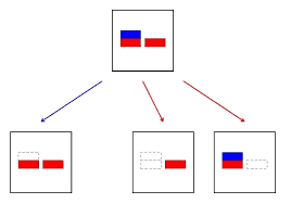
Suppose we want to perform lossy compression of some real-valued vectors, $\boldsymbol{x}n \in \mathbb{R}^D$. A very simple approach to this is to use vector quantization or VQ. The basic idea is to replace each real-valued vector $\boldsymbol{x}_n \in \mathbb{R}^D$ with a discrete symbol $z_n \in{1, \ldots, K}$, which is an index into a codebook of $K$ prototypes, $\boldsymbol{\mu}_k \in \mathbb{R}^D$. Each data vector is encoded by using the index of the most similar prototype, where similarity is measured in terms of Euclidean distance: $$ \operatorname{encode}\left(\boldsymbol{x}_n\right)=\arg \min _k\left|\boldsymbol{x}_n-\boldsymbol{\mu}_k\right|^2 $$ We can define a cost function that measures the quality of a codebook by computing the reconstruction error or distortion it induces: $$ J \triangleq \frac{1}{N} \sum{n=1}^N\left|\boldsymbol{x}n-\operatorname{decode}\left(\operatorname{encode}\left(\boldsymbol{x}_n\right)\right)\right|^2=\frac{1}{N} \sum{n=1}^N\left|\boldsymbol{x}n-\boldsymbol{\mu}{z_n}\right|^2
$$
where decode $(k)=\boldsymbol{\mu}_k$. This is exactly the cost function that is minimized by the K-means algorithm. Of course, we can achieve zero distortion if we assign one prototype to every data vector, by using $K=N$ and assigning $\boldsymbol{\mu}_n=\boldsymbol{x}_n$. However, this does not compress the data at all. In particular, it takes $O(N D B)$ bits, where $N$ is the number of real-valued data vectors, each of length $D$, and $B$ is the number of bits needed to represent a real-valued scalar (the quantization accuracy to represent each $\left.\boldsymbol{x}_n\right)$

We can do better by detecting similar vectors in the data, creating prototypes or centroids for them, and then representing the data as deviations from these prototypes. This reduces the space requirement to $O\left(N \log _2 K+K D B\right)$ bits. The $O\left(N \log _2 K\right)$ term arises because each of the $N$ data vectors needs to specify which of the $K$ codewords it is using; and the $O(K D B)$ term arises because we have to store each codebook entry, each of which is a $D$-dimensional vector. When $N$ is large, the first term dominates the second, so we can approximate the rate of the encoding scheme (number of bits needed per object) as $O\left(\log _2 K\right)$, which is typically much less than $O(D B)$.

One application of VQ is to image compression. Consider the $200 \times 320$ pixel image in Figure $21.9$; we will treat this as a set of $N=64,000$ scalars. If we use one byte to represent each pixel (a gray-scale intensity of 0 to 255 ), then $B=8$, so we need $N B=512,000$ bits to represent the image in uncompressed form. For the compressed image, we need $O\left(N \log _2 K\right)$ bits. For $K=4$, this is about $128 \mathrm{~kb}$, a factor of 4 compression, yet it results in negligible perceptual loss (see Figure 21.9(b)). Greater compression could be achieved if we modeled spatial correlation between the pixels, e.g., if we encoded $5 \times 5$ blocks (as used by JPEG). This is because the residual errors (differences from the connection between data compression and density estimation. See the sequel to this book, [Mur22], for more information.

计算机代写|机器学习代写machine learning代考|The K-means++ algorithm

K-means is optimizing a non-convex objective, and hence needs to be initialized carefully. A simple approach is to pick $K$ data points at random, and to use these as the initial values for $\boldsymbol{\mu}_k$. We can improve on this by using multiple restarts, i.e., we run the algorithm multiple times from different random starting points, and then pick the best solution. However, this can be slow.

A better approach is to pick the centers sequentially so as to try to “cover” the data. That is, we pick the initial point uniformly at random, and then each subsequent point is picked from the remaining points, with probability proportional to its squared distance to the point’s closest cluster center. That is, at iteration $t$, we pick the next cluster center to be $\boldsymbol{x}n$ with probability $$ p\left(\boldsymbol{\mu}_t=\boldsymbol{x}_n\right)=\frac{D{t-1}\left(\boldsymbol{x}n\right)}{\sum{n^{\prime}=1}^N D_{t-1}\left(\boldsymbol{x}{n^{\prime}}\right)} $$ where $$ D_t(\boldsymbol{x})=\min {k=1}^{t-1}\left|\boldsymbol{x}-\boldsymbol{\mu}_k\right|_2^2
$$
is the squared distance of $\boldsymbol{x}$ to the closest existing centroid. Thus points that are far away from a centroid are more likely to be picked, thus reducing the distortion. This is known as farthest point clustering [Gon85], or K-means++ [AV07; Bah+12; Bac+16; BLK17; LS19a]. Surprisingly, this simple trick can be shown to guarantee that the recontruction error is never more than $O(\log K)$ worse than optimal [AV07].

机器学习代考

计算机代写|机器学习代写machine learning代考|Vector quantization

假设我们要对一些实值向量进行有损压缩， $x n \in \mathbb{R}^D$.一种非常简单的方法是使用矢量量化或 $V Q_{\text {。基本思想是 }}$ 替换每个实值向量 $\boldsymbol{x}_n \in \mathbb{R}^D$ 带有离散符号 $z_n \in 1, \ldots, K$ ，这是一个密码本的索引 $K$ 原型， $\boldsymbol{\mu}_k \in \mathbb{R}^D$. 每个数据向量都使用最相似原型的索引进行编码，其中相似性根据欧氏距离来衡量:
$$
\operatorname{encode}\left(\boldsymbol{x}_n\right)=\arg \min _k\left|\boldsymbol{x}_n-\boldsymbol{\mu}_k\right|^2
$$
我们可以定义一个成本函数，通过计算它引起的重构误差或失真来衡量码本的质量:
$$
J \triangleq \frac{1}{N} \sum n=1^N\left|\boldsymbol{x} n-\operatorname{decode}\left(\operatorname{encode}\left(\boldsymbol{x}_n\right)\right)\right|^2=\frac{1}{N} \sum n=1^N\left|\boldsymbol{x} n-\boldsymbol{\mu} z_n\right|^2
$$
在哪里解码 $(k)=\boldsymbol{\mu}_k$. 这正是 K-means 算法最小化的成本函数。当然，如果我们为每个数据向量分配一个原型，我们可以实现零失真，通过使用 $K=N$ 并分配 $\boldsymbol{\mu}_n=\boldsymbol{x}_n$. 但是，这根本不会压缩数据。特别是，它需要 $O(N D B)$ 位，其中 $N$ 是实值数据向量的数量，每个向量的长度 $D$ ，和 $B$ 是表示实数值标量所需的位数（表示每个标量的量化精度 $\left.\boldsymbol{x}_n\right)$
我们可以通过检测数据中的相似向量，为它们创建原型或质心，然后将数据表示为与这些原型的偏差来做得更好。这减少了空间需求 $O\left(N \log _2 K+K D B\right)$ 位。这 $O\left(N \log _2 K\right)$ 术语出现是因为每个 $N$ 数据向量需要指定哪一个 $K$ 它正在使用的代码字；和 $O(K D B)$ 出现术语是因为我们必须存储每个密码本条目，每个条目都是一个 $D$ 维向量。什么时候 $N$ 很大，第一项支配第二项，因此我们可以将编码方案的速率 (每个对象所需的位数) 近似为 $O\left(\log _2 K\right)$ ，这通常远小于 $O(D B)$.
VQ 的一个应用是图像压缩。考虑 $200 \times 320$ 图中的像素图像 $21.9$; 我们将把它当作一组 $N=64,000$ 标量。如果我们用一个字节来表示每个像素 (灰度强度为 0 到 255 ) ，那么 $B=8$ ，所以我们需要 $N B=512,000$ 以末压缩形式表示图像的位。对于压缩图像，我们需要 $O\left(N \log _2 K\right)$ 位。为了 $K=4$ ，这是关于 $128 \mathrm{~kb}$ ，一个 4 倍的压缩因子，但它导致的感知损失可以忽略不计（见图 $21.9$ (b) ) 。如果我们对像素之间的空间相关性进行建模，例如，如果我们编码，则可以实现更大的压缩 $5 \times 5$ 块（由JPEG 使用)。这是因为残差 (不同于数据压缩和密度估计之间的联系。有关更多信息，请参阅本书的续集 [Mur22]。

计算机代写|机器学习代写machine learning代考|The K-means++ algorithm

K-means 正在优化一个非凸目标，因此需要仔细初始化。一个简单的方法是选择 $K$ 随机数据点，并使用这些作为初始值 $\boldsymbol{\mu}k$. 我们可以通过使用多次重新启动来改进这一点，即我们从不同的随机起点多次运行算法，然后选择最佳解决方案。但是，这可能很慢。更好的方法是按顺序选择中心以尝试”覆盖”数据。也就是说，我们随机均匀地选择初始点，然后从剩余的点中选择每个后续点，概率与其到该点最近的聚类中心的距离的平方成正比。也就是说，在迭代 $t$ ，我们选择下一个聚类中心 $\boldsymbol{x} n$ 有概率 $$ p\left(\boldsymbol{\mu}_t=\boldsymbol{x}_n\right)=\frac{D t-1(\boldsymbol{x} n)}{\sum n^{\prime}=1^N D{t-1}\left(\boldsymbol{x} n^{\prime}\right)}
$$
在哪里
$$
D_t(\boldsymbol{x})=\min k=1^{t-1}\left|\boldsymbol{x}-\boldsymbol{\mu}_k\right|_2^2
$$
是的平方距离 $\boldsymbol{x}$ 到最近的现有质心。因此远离质心的点更有可能被拾取，从而减少失真。这被称为最远点聚类 [Gon85]，或 K-means++ [AV07；呸+12；背+16；BLK17；LS19a]。令人惊讶的是，这个简单的技巧可以保证重构误差永远不会超过 $O(\log K)$ 比最优 [AV07] 更差。

计算机代写|机器学习代写machine learning代考请认准statistics-lab™

统计代写请认准statistics-lab™. statistics-lab™为您的留学生涯保驾护航。

金融工程代写

金融工程是使用数学技术来解决金融问题。金融工程使用计算机科学、统计学、经济学和应用数学领域的工具和知识来解决当前的金融问题，以及设计新的和创新的金融产品。

非参数统计代写

非参数统计指的是一种统计方法，其中不假设数据来自于由少数参数决定的规定模型；这种模型的例子包括正态分布模型和线性回归模型。

广义线性模型代考

广义线性模型（GLM）归属统计学领域，是一种应用灵活的线性回归模型。该模型允许因变量的偏差分布有除了正态分布之外的其它分布。

术语广义线性模型（GLM）通常是指给定连续和/或分类预测因素的连续响应变量的常规线性回归模型。它包括多元线性回归，以及方差分析和方差分析（仅含固定效应）。

有限元方法代写

有限元方法（FEM）是一种流行的方法，用于数值解决工程和数学建模中出现的微分方程。典型的问题领域包括结构分析、传热、流体流动、质量运输和电磁势等传统领域。

有限元是一种通用的数值方法，用于解决两个或三个空间变量的偏微分方程（即一些边界值问题）。为了解决一个问题，有限元将一个大系统细分为更小、更简单的部分，称为有限元。这是通过在空间维度上的特定空间离散化来实现的，它是通过构建对象的网格来实现的：用于求解的数值域，它有有限数量的点。边界值问题的有限元方法表述最终导致一个代数方程组。该方法在域上对未知函数进行逼近。[1] 然后将模拟这些有限元的简单方程组合成一个更大的方程系统，以模拟整个问题。然后，有限元通过变化微积分使相关的误差函数最小化来逼近一个解决方案。

tatistics-lab作为专业的留学生服务机构，多年来已为美国、英国、加拿大、澳洲等留学热门地的学生提供专业的学术服务，包括但不限于Essay代写，Assignment代写，Dissertation代写，Report代写，小组作业代写，Proposal代写，Paper代写，Presentation代写，计算机作业代写，论文修改和润色，网课代做，exam代考等等。写作范围涵盖高中，本科，研究生等海外留学全阶段，辐射金融，经济学，会计学，审计学，管理学等全球99%专业科目。写作团队既有专业英语母语作者，也有海外名校硕博留学生，每位写作老师都拥有过硬的语言能力，专业的学科背景和学术写作经验。我们承诺100%原创，100%专业，100%准时，100%满意。

随机分析代写

随机微积分是数学的一个分支，对随机过程进行操作。它允许为随机过程的积分定义一个关于随机过程的一致的积分理论。这个领域是由日本数学家伊藤清在第二次世界大战期间创建并开始的。

时间序列分析代写

随机过程，是依赖于参数的一组随机变量的全体，参数通常是时间。随机变量是随机现象的数量表现，其时间序列是一组按照时间发生先后顺序进行排列的数据点序列。通常一组时间序列的时间间隔为一恒定值（如1秒，5分钟，12小时，7天，1年），因此时间序列可以作为离散时间数据进行分析处理。研究时间序列数据的意义在于现实中，往往需要研究某个事物其随时间发展变化的规律。这就需要通过研究该事物过去发展的历史记录，以得到其自身发展的规律。

回归分析代写

多元回归分析渐进（Multiple Regression Analysis Asymptotics）属于计量经济学领域，主要是一种数学上的统计分析方法，可以分析复杂情况下各影响因素的数学关系，在自然科学、社会和经济学等多个领域内应用广泛。

MATLAB代写

MATLAB 是一种用于技术计算的高性能语言。它将计算、可视化和编程集成在一个易于使用的环境中，其中问题和解决方案以熟悉的数学符号表示。典型用途包括：数学和计算算法开发建模、仿真和原型制作数据分析、探索和可视化科学和工程图形应用程序开发，包括图形用户界面构建MATLAB 是一个交互式系统，其基本数据元素是一个不需要维度的数组。这使您可以解决许多技术计算问题，尤其是那些具有矩阵和向量公式的问题，而只需用 C 或 Fortran 等标量非交互式语言编写程序所需的时间的一小部分。MATLAB 名称代表矩阵实验室。MATLAB 最初的编写目的是提供对由 LINPACK 和 EISPACK 项目开发的矩阵软件的轻松访问，这两个项目共同代表了矩阵计算软件的最新技术。MATLAB 经过多年的发展，得到了许多用户的投入。在大学环境中，它是数学、工程和科学入门和高级课程的标准教学工具。在工业领域，MATLAB 是高效研究、开发和分析的首选工具。MATLAB 具有一系列称为工具箱的特定于应用程序的解决方案。对于大多数 MATLAB 用户来说非常重要，工具箱允许您学习和应用专业技术。工具箱是 MATLAB 函数（M 文件）的综合集合，可扩展 MATLAB 环境以解决特定类别的问题。可用工具箱的领域包括信号处理、控制系统、神经网络、模糊逻辑、小波、仿真等。

R语言代写	问卷设计与分析代写
PYTHON代写	回归分析与线性模型代写
MATLAB代写	方差分析与试验设计代写
STATA代写	机器学习/统计学习代写
SPSS代写	计量经济学代写
EVIEWS代写	时间序列分析代写
EXCEL代写	深度学习代写
SQL代写	各种数据建模与可视化代写

经济代写|博弈论代写Game Theory代考|ECON40010

Posted on 2022年11月29日2022年11月29日 by statistics-lab

如果你也在怎样代写博弈论Game Theory这个学科遇到相关的难题，请随时右上角联系我们的24/7代写客服。

博弈论是对理性主体之间战略互动的数学模型的研究。它在社会科学的所有领域，以及逻辑学、系统科学和计算机科学中都有应用。最初，它针对的是两人的零和博弈，其中每个参与者的收益或损失都与其他参与者的收益或损失完全平衡。在21世纪，博弈论适用于广泛的行为关系；它现在是人类、动物以及计算机的逻辑决策科学的一个总称。

statistics-lab™ 为您的留学生涯保驾护航在代写博弈论Game Theory方面已经树立了自己的口碑, 保证靠谱, 高质且原创的统计Statistics代写服务。我们的专家在代写博弈论Game Theory代写方面经验极为丰富，各种代写博弈论Game Theory相关的作业也就用不着说。

我们提供的博弈论Game Theory及其相关学科的代写，服务范围广, 其中包括但不限于:

Statistical Inference 统计推断
Statistical Computing 统计计算
Advanced Probability Theory 高等概率论
Advanced Mathematical Statistics 高等数理统计学
(Generalized) Linear Models 广义线性模型
Statistical Machine Learning 统计机器学习
Longitudinal Data Analysis 纵向数据分析
Foundations of Data Science 数据科学基础

经济代写|博弈论代写Game Theory代考|Nim, Poker Nim, and the Mex Rule

In this section, we prove a sweeping statement (Theorem 1.14): Every impartial game is equivalent to some Nim heap. Note that this means a single Nim heap, even if the game itself is rather complicated, for example a general Nim position, which is a game sum of several Nim heaps. This can proved without any reference to playing Nim optimally. As we will see at the end of this section with the help of Figure 1.2, the so-called mex rule that underlies Theorem $1.14$ can be used to discover the role of powers of two for playing sums of Nim heaps.

We use the following notation for Nim heaps. If $G$ is a single Nim heap with $n$ tokens, $n \geq 0$, then we denote this game by $* n$. This game is completely specified by its $n$ options, and they are defined recursively as follows:
options of $* n: \quad * 0, * 1, * 2, \ldots, (n-1)$. Note that $ 0$ is the empty heap with no tokens, that is, $* 0=0$; we will normally continue to just write 0 .

We can use (1.18) as the definition of $* n$. For example, the game $* 4$ is defined by its options $* 0, * 1, * 2, * 3$. It is very important to include $* 0$ in that list of options, because it means that $* 4$ has a winning move. Condition (1.18) is a recursive definition of the game $* n$, because its options are also defined by reference to such games $* k$, for numbers $k$ smaller than $n$. This game fulfills the ending condition because the heap gets successively smaller in any sequence of moves.

A general Nim position is a game sum of several Nim heaps. Earlier we had written such a position by just listing the sizes of the Nim heaps, such as $1,2,3$ in (1.1). The fancy way to write this is now $* 1+* 2+* 3$, a sum of games.

The game of Poker Nim is a variation of Nim. Suppose that each player is given, at the beginning of the game, some extra “reserve” tokens. Like Nim, the game is played with heaps of tokens. In a move, a player can choose, as in ordinary Nim, a heap and remove some tokens, which he can add to his reserve tokens. A second, new kind of move is to add some of the player’s reserve tokens to some heap (or even to create an entire new heap with these tokens). These two kinds of moves are the only ones allowed.

经济代写|博弈论代写Game Theory代考|Sums of Nim Heaps

In this section, we derive how to compute the Nim value for a general Nim position, which is a sum of different Nim heaps. This will be the Nim sum that we have defined using the binary representation, now cast in the language of game sums and equivalent games, and without assuming the binary representation.

For example, we know that $* 1+* 2+* 3 \equiv 0$, so by Lemma $1.12, * 1+* 2$ is equivalent to $* 3$. In general, however, the sizes of the Nim heaps cannot simply be added to obtain the equivalent Nim heap, because $* 2+* 3$ is also equivalent to $* 1$, and $* 1+* 3$ is equivalent to $* 2$.

If $* k \equiv * n+* m$, then we call $k$ the $\operatorname{Nim}$ sum of $n$ and $m$, written $k=n \oplus m$. The following theorem states that the Nim sum of distinct powers of two is their arithmetic sum. For example, $1=2^0$ and $2=2^1$, so $1 \oplus 2=1+2=3$.

Theorem 1.15. Let $n \geq 1$, and $n=2^a+2^b+2^c+\cdots$, where $a>b>c>\cdots \geq 0$. Then
$$

n \equiv \left(2^a\right)+\left(2^b\right)+*\left(2^c\right)+\cdots \text {. }
$$
We first discuss the implications of this theorem, and then prove it. The expression $n=2^a+2^b+2^c+\cdots$ is an arithmetic sum of distinct powers of two. Any $n$ is uniquely given as such a sum. It amounts to the binary representation of $n$, which, if $n<2^{a+1}$, gives $n$ as the sum of all powers $2^a, 2^{a-1}, 2^{a-2}, \ldots, 2^0$ where each power of two is multiplied with 0 or 1 , the binary digit for the respective position. For example,
$$
9=8+1=1 \cdot 2^3+0 \cdot 2^2+0 \cdot 2^1+1 \cdot 2^0,
$$
so that 9 in decimal is written as 1001 in binary. Theorem $1.15$ uses only the distinct powers of two $2^a, 2^b, 2^c, \ldots$ that correspond to the digits 1 in the binary representation of $n$.

博弈论代考

经济代写|博弈论代写Game Theory代考|Nim, Poker Nim, and the Mex Rule

在本节中，我们证明了一个笼统的陈述（定理 1.14)：每个公正的游戏都等同于一些 Nim 堆。请注意，这意味着单个 $\mathrm{Nim}$ 堆，即使游戏本身相当复杂，例如一般的 Nim 位置，它是几个 Nim 堆的游戏总和。这可以在没有任何参考以最佳方式玩 $\operatorname{Nim}$ 的情况下证明。正如我们将在本节末尾借助图 $1.2$ 看到的，所谓的 mex 规则是定理的基础1.14可用于发现 Nim 堆求和的 2 次幂的作用。
我们对 $\operatorname{Nim}$ 堆使用以下表示法。如果 $G$ 是单个 $\operatorname{Nim}$ 堆 $n$ 代币， $n \geq 0$ ，那么我们将这个游戏表示为 $* n$. 这个游戏完全由它指定 $n$
选项，它们递归定义如下: $* n: * 0, * 1, * 2, \ldots,(n-1)$. 注意 0 是没有标记的空堆，即 $* 0=0$; 我们通常会继续只写 0 。
我们可以用 (1.18) 作为定义 $* n$. 例如，游戏 $* 4$ 由其选项定义 $* 0, * 1, * 2, * 3$. 包括在内非常重要 $* 0$ 在该选项列表中，因为这意味着 $* 4$ 有一个获胜的举动。条件 (1.18) 是游戏的递归定义 $* n$ ，因为它的选项也是通过参考此类游戏来定义的 $* k$ ，对于数字 $k$ 小于 $n$. 这个游戏满足结束条件，因为堆在任何移动序列中都逐渐变小。
一般的 $\operatorname{Nim}$ 位置是几个 $\operatorname{Nim}$ 堆的游戏总和。早些时候我们通过列出 $\operatorname{Nim}$ 堆的大小来编写这样的位置，例如 $1,2,3$ 在 (1.1) 中。现在写这个的好方法 $* 1+* 2+* 3$ ，游戏总和。
Poker Nim 游戏是 Nim 的变体。假设在游戏开始时给每个玩家一些额外的“保留”标记。与 Nim 一样，该游戏是用大量代币玩的。在移动中，玩家可以像在普通 Nim 中一样选择一个堆并移除一些令牌，他可以将这些令牌添加到他的储备令牌中。第二种新的移动方式是将玩家的一些储备令牌添加到一些堆中（或者甚至用这些令牌创建一个全新的堆）。这两种动作是唯一允许的。

经济代写|博弈论代写Game Theory代考|Sums of Nim Heaps

在本节中，我们将推导如何计算一般 Nim 位置的 $\mathrm{Nim}$ 值，该位置是不同 $\mathrm{Nim}$ 堆的总和。这将是我们使用二进制表示定义的 Nim 和，现在用游戏总和和等效游戏的语言进行转换，并且不假设二进制表示。
例如，我们知道 $* 1+* 2+* 3 \equiv 0$, 所以由引理 $1.12, * 1+* 2$ 相当于 $* 3$. 然而，一般来说， $\operatorname{Nim}$ 堆的大小不能简单地相加以获得等效的 $\operatorname{Nim}$ 堆，因为 $* 2+* 3$ 也相当于 $* 1$ ，和 $* 1+* 3$ 相当于 $* 2$.
如果 $* k \equiv * n+* m$ ，然后我们称 $k$ 这 $\mathrm{Nim}$ 的总和 $n$ 和 $m$, 写 $k=n \oplus m$. 下面的定理表明，两个不同幕的 $\operatorname{Nim}$ 和是它们的算术和。例如， $1=2^0$ 和 $2=2^1$ ，所以 $1 \oplus 2=1+2=3$.
定理 1.15。让 $n \geq 1$ ，和 $n=2^a+2^b+2^c+\cdots$ ，在哪里 $a>b>c>\cdots \geq 0$. 然后 $\$ \$$
Wefirstdiscusstheimplicationsofthistheorem, andthenproveit. Theexpression $\$ n=2$
$9=8+1=1 \backslash c$ dot $2^{\wedge} 3+0 \backslash c$ dot $2^{\wedge} 2+0 \backslash c$ dot $2^{\wedge} 1+1 \backslash c$ dot $2^{\wedge} 0$,
$\$ \$$
这样十进制的9写成二进制的 1001。定理 $1.15$ 只使用两个不同的权力 $2^a, 2^b, 2^c, \ldots$ 对应于二进制表示中的数字 $1 n$.

经济代写|博弈论代写Game Theory代考请认准statistics-lab™

统计代写请认准statistics-lab™. statistics-lab™为您的留学生涯保驾护航。

金融工程代写

非参数统计代写

非参数统计指的是一种统计方法，其中不假设数据来自于由少数参数决定的规定模型；这种模型的例子包括正态分布模型和线性回归模型。

广义线性模型代考

广义线性模型（GLM）归属统计学领域，是一种应用灵活的线性回归模型。该模型允许因变量的偏差分布有除了正态分布之外的其它分布。

有限元方法代写

随机分析代写

时间序列分析代写

回归分析代写

MATLAB代写

R语言代写	问卷设计与分析代写
PYTHON代写	回归分析与线性模型代写
MATLAB代写	方差分析与试验设计代写
STATA代写	机器学习/统计学习代写
SPSS代写	计量经济学代写
EVIEWS代写	时间序列分析代写
EXCEL代写	深度学习代写
SQL代写	各种数据建模与可视化代写

经济代写|博弈论代写Game Theory代考|ECOS3012

Posted on 2022年11月29日2022年11月29日 by statistics-lab

如果你也在怎样代写博弈论Game Theory这个学科遇到相关的难题，请随时右上角联系我们的24/7代写客服。

我们提供的博弈论Game Theory及其相关学科的代写，服务范围广, 其中包括但不限于:

Statistical Inference 统计推断
Statistical Computing 统计计算
Advanced Probability Theory 高等概率论
Advanced Mathematical Statistics 高等数理统计学
(Generalized) Linear Models 广义线性模型
Statistical Machine Learning 统计机器学习
Longitudinal Data Analysis 纵向数据分析
Foundations of Data Science 数据科学基础

经济代写|博弈论代写Game Theory代考|Top-down Induction

When talking about combinatorial games, we will often use for brevity the word game for “game position”. Every game $G$ has finitely many options $G_1, \ldots, G_m$ that are reached from $G$ by one of the allowed moves in $G$, as in this picture:

If $m=0$ then $G$ has no options. We denote the game with no options by 0 , which by the normal play convention is a losing game. Otherwise the options of $G$ are themselves games, defined by their respective options according to the rules of the game. In that way, any game is completely defined by its options. In short, the starting position defines the game completely.

We introduce a certain type of mathematical induction for games, which is applied to a partial order (see the background material text box on the next page).
Consider a set $S$ of games, defined, for example, by a starting game and all the games that can reached from it via any sequence of moves of the players. For two games $G$ and $H$ in $S$, call $H$ simpler than $G$ if there is a sequence of moves that leads from $G$ to $H$. We allow $G=H$ where this sequence is empty. The relation of being “simpler than” defines a partial order which for the moment we denote by $\leq$. Note that $\leq$ is antisymmetric because it is not possible to reach $G$ from $G$ by a nonempty sequence of moves because this would violate the ending condition. The ending condition for games implies the following property:
Every nonempty subset of $S$ has a minimal element.
If there was a nonempty subset $T$ of $S$ without a minimal element, then we could produce an infinite play as follows: Start with some $G$ in $T$. Because $G$ is not minimal, there is some $H$ in $T$ with $H<G$, so there is some sequence of moves from $G$ to $H$. Similarly, $H$ is not minimal, so another game in $T$ is reached from $H$. Continuing in this manner creates an infinite sequence of moves, which contradicts the ending condition.

经济代写|博弈论代写Game Theory代考|Game Sums and Equivalence of Games

Combinatorial games often “decompose” into parts in which players can move independently, and the players then have to decide in which part to make their move. This is captured by the important concept of a sum of games.

Definition 1.4. Suppose that $G$ and $H$ are game positions with options (positions reached by one move) $G_1, \ldots, G_k$ and $H_1, \ldots, H_m$, respectively. Then the options of the game sum $G+H$ are
$$
G_1+H, \ldots, G_k+H, \quad G+H_1, \ldots, G+H_m .
$$
The first list of options $G_1+H, \ldots, G_k+H$ in (1.11) simply means that the player makes his move in $G$, the second list $G+H_1, \ldots, G+H_m$ that he makes his move in $H$; the other part of the game sum remains untouched. As an example, a Nim position is simply the game sum of its individual Nim heaps, because the player moves in exactly one of the heaps.

Definition $1.4$ is a recursive definition, because the game sum is defined in terms of its options, which are themselves game sums (but they are simpler games).
The sum of games turns out to define an abelian group on the (appropriately defined) set of games. It is a commutative and associative operation: for any games $\mathrm{G}, H, J$,
$$
G+H=H+G \text { and }(G+H)+J=G+(H+J) \text {. }
$$
The first condition (commutativity) holds because the order of the options of a game, used in (1.11), does not matter. The second condition (associativity) holds because both $(G+H)+J$ and $G+(H+J)$ mean in effect that the player decides to move in $G$, in $H$, or in $J$, leaving the other two parts of the game sum unchanged. We can therefore assume the equalities (1.12). More generally, in a sum of several games $G_1, \ldots, G_n$ the player moves in exactly one of these games, which does not depend on how these games are arranged, so that we can write this sum unambiguously without parentheses as $G_1+\cdots+G_n$.

The losing game 0 which has no options is a zero (neutral element) for game sums: It fulfills $G+0=G$ for any game $G$, because the game 0 is “invisible” when added to $G$.

In order to obtain a group, every game $G$ needs to have a “negative” game $-G$ so that $G+(-G)=0$. However, this equality cannot hold as stated as soon as the game $G$ has options, because then the game $G+(-G)$ also has options but 0 has none. Instead, we need a more general condition
$$
G+(-G) \equiv 0,
$$
where $G \equiv H$ means that the two games $G$ and $H$ are equivalent, according to the following definition.

博弈论代考

经济代写|博弈论代写Game Theory代考|Top-down Induction

在谈论组合游戏时，为简洁起见，我们经常使用“游戏位置”这个词来表示游戏。每场比㥶 $G$ 有有限多个选项 $G_1, \ldots, G_m$ 从 $G$ 通过允许的移动之- $G$ ，就像这张图:
如果 $m=0$ 然后 $G$ 没有选择。我们用 0 表示没有选项的游戏，按照正常的游戏惯例，这是一场失败的游戏。否则选项 $G$ 它们本身就是游戏，根据游戏规则由各自的选项定义。这样，任何游戏都完全由其选项定义。简而言之，起始位置完全定义了游戏。
我们介绍了一种特定类型的游戏数学归纳法，它适用于偏序（见下一页的背景材料文本框)。
考虑一组S游戏的定义，例如，由一个开始游戏和所有可以通过玩家的任何移动顺序从它到达的游戏来定义。对于两场比寒 $G$ 和 $H$ 在 $S$ ，称呼 $H$ 比 $G$ 如果有一系列动作导致 $G$ 至 $H$. 我们允许 $G=H$ 这个序列是空的。”比”更简单的关系定义了一个偏序，目前我们用 $\leq$. 注意 $\leq$ 是反对称的，因为不可能到达 $G$ 从 $G$ 通过一个非空的移动序列，因为这会违反结束条件。游戏的结束条件意味着以下属性
: $S$ 有一个最小的元素。
如果有一个非空子集 $T$ 的 $S$ 如果没有最小元素，那么我们可以产生一个无限游戏，如下所示：从一些开始 $G$ 在 $T$. 因为 $G$ 不是最小的，有一些 $H$ 在 $T$ 和 $H<G$ ，所以有一些移动顺序 $G$ 至 $H$. 相似地， $H$ 不是最小的，所以另一个游戏 $T$ 从 $H$. 以这种方式继续下去会产生无限的移动序列，这与结束条件相矛盾。

经济代写|博弈论代写Game Theory代考|Game Sums and Equivalence of Games

组合博栾通常会”分解”成玩家可以独立移动的部分，然后玩家必须决定在哪一部分移动。博弈总和这一重要概念体现了这一点。
定义 1.4。假设 $G$ 和 $H$ 是带有选项的游戏位置 (一步到达的位置) $G_1, \ldots, G_k$ 和 $H_1, \ldots, H_m$ ，分别。然后游戏总和的选项 $G+H$ 是
$$
G_1+H, \ldots, G_k+H, \quad G+H_1, \ldots, G+H_m .
$$
第一个选项列表 $G_1+H, \ldots, G_k+H$ 在 (1.11) 中只是意味着玩家在 $G$ ，第二个列表 $G+H_1, \ldots, G+H_m$ 他搬进来 $H$; 游戏总和的另一部分保持不变。例如，一个 $\mathrm{Nim}$ 位置只是其各个 $\mathrm{Nim}$ 堆的游戏总和，因为玩家恰好在其中一个堆中移动。
定义 1.4是一个递归定义，因为游戏总和是根据其选项定义的，这些选项本身就是游戏总和（但它们是更简单的游戏)。。
游戏的总和在（适当定义的）游戏集上定义了一个阿贝尔群。它是一种交换结合运算：对于任何游戏G, $H, J$ ，
$$
G+H=H+G \text { and }(G+H)+J=G+(H+J) .
$$
第一个条件 (交换性) 成立是因为 (1.11) 中使用的游戏选项的顺序无关紧要。第二个条件 (关联性) 成立，因为两者 $(G+H)+J$ 和 $G+(H+J)$ 实际上意味着玩家决定搬进来 $G$ ，在 $H$ ，或者在 $J$ ，游戏总和的其他两部分保持不变。因此，我们可以假设等式 (1.12)。更一般地，在几个游戏的总和中 $G_1, \ldots, G_n$ 玩家恰好在这些游戏中的一个中移动，这与这些游戏的排列方式无关，因此我们可以在没有括号的情况下明确地将这个总和写为 $G_1+\cdots+G_n$.
没有选项的失败游戏 0 是游戏总和的零 (中性元素) : 它满足 $G+0=G$ 对于任何游戏 $G$ ，因为游戏 0 在添加到时是“不可见的” $G$.
为了获得一个团体，每场比䗙 $G$ 需要有一个”消极”的游戏 $-G$ 以便 $G+(-G)=0$. 然而，这种平等不能像游戏中所说的那样成立 $G$ 有选项，因为那时游戏 $G+(-G)$ 也有选项，但 0 没有。相反，我们需要一个更一般的条件
$$
G+(-G) \equiv 0,
$$
在挪里 $G \equiv H$ 意味着这两款游戏 $G$ 和 $H$ 根据以下定义，它们是等价的。

统计代写请认准statistics-lab™. statistics-lab™为您的留学生涯保驾护航。

金融工程代写

非参数统计代写

非参数统计指的是一种统计方法，其中不假设数据来自于由少数参数决定的规定模型；这种模型的例子包括正态分布模型和线性回归模型。

广义线性模型代考

广义线性模型（GLM）归属统计学领域，是一种应用灵活的线性回归模型。该模型允许因变量的偏差分布有除了正态分布之外的其它分布。

有限元方法代写

随机分析代写

时间序列分析代写

回归分析代写

MATLAB代写

R语言代写	问卷设计与分析代写
PYTHON代写	回归分析与线性模型代写
MATLAB代写	方差分析与试验设计代写
STATA代写	机器学习/统计学习代写
SPSS代写	计量经济学代写
EVIEWS代写	时间序列分析代写
EXCEL代写	深度学习代写
SQL代写	各种数据建模与可视化代写

经济代写|博弈论代写Game Theory代考|ECON6025

Posted on 2022年11月29日2022年11月29日 by statistics-lab

如果你也在怎样代写博弈论Game Theory这个学科遇到相关的难题，请随时右上角联系我们的24/7代写客服。

我们提供的博弈论Game Theory及其相关学科的代写，服务范围广, 其中包括但不限于:

Statistical Inference 统计推断
Statistical Computing 统计计算
Advanced Probability Theory 高等概率论
Advanced Mathematical Statistics 高等数理统计学
(Generalized) Linear Models 广义线性模型
Statistical Machine Learning 统计机器学习
Longitudinal Data Analysis 纵向数据分析
Foundations of Data Science 数据科学基础

经济代写|博弈论代写Game Theory代考|Nim and Combinatorial Games

Combinatorial game theory is about perfect-information two-player games, such as Checkers, Go, Chess, or Nim, which are analyzed using their rules. It tries to answer who will win in a game position (assuming optimal play on both sides), and to quantify who is ahead and by how much. The topic has a rich mathematical theory that relates to discrete mathematics, algebra, and (not touched here) computational complexity, and highly original ideas specific to these games.
Combinatorial games are not part of “classical” game theory as used in economics. However, they nicely demonstrate that game theory is about rigorous, and often unfamiliar, mathematical concepts rather than complex techniques.
This chapter is only an introduction to combinatorial games. It presents the theory of impartial games where in any game position both players have the same allowed moves. We show the powerful and surprisingly simple result (Theorem 1.14), independently found by Sprague (1935) and Grundy (1939), that every impartial game is equivalent to a “Nim heap” of suitable size.

In Section $1.8$ we give a short glimpse into the more general theory of partizan games, where the allowed moves may depend on the player (e.g., one player can move the white pieces on the game board and the other player the black pieces).
For a deeper treatment, the final Section $1.9$ of this chapter lists some excellent textbooks on combinatorial games. They treat impartial games as a special case of general combinatorial games. In contrast, we first treat the simpler impartial games in full.

经济代写|博弈论代写Game Theory代考|Prerequisites and Learning Outcomes

Combinatorial games are two-player win-lose games of perfect information, that is, every player is perfectly informed about the state of play (unlike, for example, the card games Bridge or Poker that have hidden information). The games do not have chance moves like rolling dice or shuffling cards. When playing the game, the two players always alternate in making a move. Every play of the game ends with a win for one player and a loss for the other player (some games like Chess allow for a draw as an outcome, but not the games we consider here).

The game has a (typically finite) number of positions, with well-defined rules that define the allowed moves to reach the next position. The rules are such that play will always come to an end because some player is unable to move. This is called the ending condition. We assume the normal play convention that a player unable to move loses. The alternative to normal play is misère play, where a player who is unable to move wins (so the previous player who has made the last move loses).

We study impartial games where the available moves in a game position do not depend on whose turn it is to move. If that is not the case, as in Chess where one player can only move the white pieces and the other player the black pieces, the game is called partizan.

For impartial games, the game Nim plays a central role. A game position in Nim is given by some heaps of tokens, and a move is to remove some (at least one, possibly all) tokens from one of the heaps. The last player able to move wins the game, according to the normal play convention.

We analyze the Nim position 1,2,3, which means three heaps with one, two, and three tokens, respectively. One possible move is to remove two tokens from the heap of size three, like here: which we write as a move from $1,2,3$ to $1,2,1$. Because the move can be made in any one heap, the order of the heap sizes does not matter, so the position $1,2,1$ could also be written as $1,1,2$. The options of a game position are the positions that can be reached by a single legal move (according to the game rules) from the player to move. We draw them with moves shown as downward lines, like here,

where the first option 2,3 is obtained by removing from $1,2,3$ the entire heap of size 1 , the second option 1,1,3 by removing one token from the heap of size 2 , and so on. The game tree is obtained by continuing to draw all possible moves in this way until play ends (game trees are studied in much more detail in Chapter 4). We may conflate options with obvious equal meaning, such as the positions 1,1,2 and 1,2,1 that can be reached from 1,2,2. However, we do not draw moves to the same position from two different predecessors, such as 1,1,2 that can be reached from $1,1,3$ and 1, 2,2. Instead, such a position like 1,1,2 will be repeated in the game tree, so that every position has a unique history of moves.

In an impartial game, the available moves in a game position are by definition independent of the player to move. A game position belongs therefore to exactly one of two possible outcome classes, namely it is either a winning or a losing position. “Winning” or “losing” applies to the player whose turn it is to move, assuming optimal play. A winning position means that the player can force a win with a suitable first “winning” move (and subsequent winning moves at all later positions). A losing position means that every move from the current position leads to a winning position of the other player, who can then force a win, so that the current player will lose.

博弈论代考

经济代写|博弈论代写Game Theory代考|Nim and Combinatorial Games

组合博弈论是关于完美信息的两人游戏，例如西洋跳棋、围棋、国际象棋或 Nim，这些游戏使用它们的规则进行分析。它试图回答谁将在比赛中获胜（假设双方都发挥最佳状态），并量化谁领先以及领先多少。该主题具有丰富的数学理论，涉及离散数学、代数和（此处未涉及）计算复杂性，以及针对这些游戏的高度原创的想法。
组合博弈不是经济学中使用的“经典”博弈论的一部分。然而，它们很好地证明博弈论是关于严格的、通常是陌生的数学概念，而不是复杂的技术。
本章只是对组合博弈的介绍。它提出了公平游戏的理论，即在任何游戏位置上，两个玩家都有相同的允许移动。我们展示了由 Sprague (1935) 和 Grundy (1939) 独立发现的强大而简单的结果（定理 1.14），即每个公正的游戏都等同于一个合适大小的“Nim 堆”。

在节1.8我们简要介绍了党派游戏的更一般理论，其中允许的移动可能取决于玩家（例如，一个玩家可以移动游戏板上的白色棋子，另一个玩家可以移动黑色棋子）。
为了更深入的处理，最后一节1.9本章的末尾列出了一些关于组合博弈的优秀教科书。他们将无偏博弈视为一般组合博弈的特例。相比之下，我们首先全面对待更简单的公平博弈。

经济代写|博弈论代写Game Theory代考|Prerequisites and Learning Outcomes

组合游戏是完美信息的双人输赢游戏，也就是说，每个玩家都完全了解游戏的状态（不像，例如，具有隐藏信息的纸牌游戏 Bridge 或 Poker）。游戏没有像掷骰子或洗牌这样的机会动作。下棋时，两位棋手总是交替着手。游戏的每一局比赛都以一个玩家获胜而另一个玩家失败而告终（某些游戏，如国际象棋允许平局作为结果，但我们在这里考虑的游戏则不允许）。

游戏有一个（通常是有限的）位置，具有定义明确的规则，这些规则定义了到达下一个位置的允许移动。规则是这样的，比赛总会结束，因为有些球员无法移动。这称为结束条件。我们假设无法移动的玩家输了的正常游戏规则。正常游戏的另一种选择是 misère 游戏，无法移动的玩家获胜（因此最后一步的玩家输了）。

我们研究公平游戏，其中游戏位置的可用移动不取决于轮到谁移动。如果不是这种情况，就像在国际象棋中一个玩家只能移动白色棋子而另一个玩家只能移动黑色棋子一样，该游戏称为游击队。

对于公平游戏，Nim 游戏起着核心作用。Nim 中的游戏位置由一些令牌堆给出，移动是从其中一个堆中移除一些（至少一个，可能是全部）令牌。根据正常的游戏规则，最后一个能够移动的玩家获胜。

我们分析 Nim 位置 1,2,3，这意味着三个堆分别有一个、两个和三个令牌。一种可能的移动是从大小为 3 的堆中删除两个标记，如下所示：我们将其写为移动1,2,3至1,2,1. 因为移动可以在任何一个堆中进行，堆大小的顺序无关紧要，所以位置1,2,1也可以写成1,1,2. 游戏位置的选项是玩家通过一次合法移动（根据游戏规则）可以到达的位置。我们用向下的线表示的移动来绘制它们，就像这里一样，

其中第一个选项 2,3 是通过从1,2,3大小为 1 的整个堆，第二个选项 1,1,3 通过从大小为 2 的堆中删除一个标记，依此类推。以这种方式继续画出所有可能的走法，直到游戏结束，即可获得博弈树（博弈树在第 4 章中有更详细的研究）。我们可能会将具有明显相同含义的选项混为一谈，例如可以从 1,2,2 到达的位置 1,1,2 和 1,2,1。但是，我们不会从两个不同的前辈绘制移动到相同的位置，例如可以从中到达的 1,1,21,1,3和 1、2、2。相反，像 1,1,2 这样的位置将在博弈树中重复出现，因此每个位置都有唯一的移动历史。

在公平游戏中，根据定义，游戏位置中的可用移动与玩家移动无关。因此，游戏位置恰好属于两个可能的结果类别之一，即它要么是获胜位置，要么是失败位置。假设最佳游戏，“获胜”或“失败”适用于轮到该移动的玩家。获胜的位置意味着玩家可以通过合适的第一个“获胜”动作（以及随后所有后续位置的获胜动作）来迫使获胜。失败的位置意味着从当前位置开始的每一步都会导致其他玩家的获胜位置，然后其他玩家可以强制获胜，这样当前玩家就会输。

统计代写请认准statistics-lab™. statistics-lab™为您的留学生涯保驾护航。

金融工程代写

非参数统计代写

非参数统计指的是一种统计方法，其中不假设数据来自于由少数参数决定的规定模型；这种模型的例子包括正态分布模型和线性回归模型。

广义线性模型代考

广义线性模型（GLM）归属统计学领域，是一种应用灵活的线性回归模型。该模型允许因变量的偏差分布有除了正态分布之外的其它分布。

有限元方法代写

随机分析代写

时间序列分析代写

回归分析代写

MATLAB代写

R语言代写	问卷设计与分析代写
PYTHON代写	回归分析与线性模型代写
MATLAB代写	方差分析与试验设计代写
STATA代写	机器学习/统计学习代写
SPSS代写	计量经济学代写
EVIEWS代写	时间序列分析代写
EXCEL代写	深度学习代写
SQL代写	各种数据建模与可视化代写

统计代写|随机过程代写stochastic process代考|MTH7090

Posted on 2022年11月28日2022年11月28日 by statistics-lab

如果你也在怎样代写随机过程stochastic process这个学科遇到相关的难题，请随时右上角联系我们的24/7代写客服。

随机过程 用于表示在时间上发展的统计现象以及在处理这些现象时出现的理论模型，由于这些现象在许多领域都会遇到，因此这篇文章具有广泛的实际意义。

statistics-lab™ 为您的留学生涯保驾护航在代写随机过程stochastic process方面已经树立了自己的口碑, 保证靠谱, 高质且原创的统计Statistics代写服务。我们的专家在代写随机过程stochastic process代写方面经验极为丰富，各种代写随机过程stochastic process相关的作业也就用不着说。

我们提供的随机过程stochastic process及其相关学科的代写，服务范围广, 其中包括但不限于:

Statistical Inference 统计推断
Statistical Computing 统计计算
Advanced Probability Theory 高等概率论
Advanced Mathematical Statistics 高等数理统计学
(Generalized) Linear Models 广义线性模型
Statistical Machine Learning 统计机器学习
Longitudinal Data Analysis 纵向数据分析
Foundations of Data Science 数据科学基础

统计代写|随机过程代写stochastic process代考|Special Chains and Foster Type Theorems

If the Markov Chain is infinite, the number of equations given by $\pi(P-I)=0$ will be infinite involving an infinite number of unknowns. In some particular cases we can solve these equations. The following examples will illustrate this point.
Example 2.5 Birth and-Death Chain (Non-Homogeneous Random Walk) Consider a birth and death chain on ${0,1,2, \ldots, d}$ or a set of non-negative integers i.e. where $d=\infty$. Assume that the chain is irreducible i.e. $p_j>0$ and $q_j>0$ in case $0 \leq j \leq d$ (i.e. when $d$ is finite) $p_j>0$ for $0 \leq j<\infty$ and $q_j>0$ for $0<j<\infty$ if $d$ is infinite. Consider the transition matrix when $d<\infty$ we assume that $r_i=0$ for $i \geq 0$ and $p_0=1$.
Particular Case: First consider that $d$ is still infinite and $r_1=0$ for $i \geq 0$, $p_0=1$. The stationary distribution is given by

$$
X=\left(x_0, x_1, x_2, \ldots\right)=\left(x_0, x_1, x_2, \ldots\right)\left(\begin{array}{ccccc}
0 & 1 & 0 & 0 & \ldots \
q_1 & 0 & p_1 & 0 & \ldots \
0 & q_2 & 0 & p_2 & \cdots
\end{array}\right)
$$
or $X=X P$. Let $x_0 \neq 0$. Then
$$
\begin{aligned}
&x_0=x_1 q_1, \
&x_1=x_0+x_2 q_2, \
&x_3=x_2 p_2+x_4 q_4, \
&x_4=\ldots \
&\cdots
\end{aligned}
$$
Define
Then
$$
y_i=\frac{x_i}{x_0}, y_0=1, i=1,2,3, \ldots
$$
$$
\begin{aligned}
&y_1=1 / q_1, y_1=1+y_2 q_2 \text { or } y_2=\frac{y_1-1}{q_2}=\frac{1-q_1}{q_1 q_2}=\frac{p_1}{q_1 q_2} \
&y_3=\frac{p_1 p_2}{q_1 q_2 q_3}, \ldots, y_n=\frac{p_1 p_2 \ldots p_{n-1}}{q_1 q_2 \ldots q_n}>0 \quad \text { for all } n=1,2, \ldots
\end{aligned}
$$
(by assumption that all $p, q$ ‘s are $>0$ ).

统计代写|随机过程代写stochastic process代考|Foster type theorems

The following theorems, associated with Foster, give criteria for transient and recurrent chains in terms of solution of certain equations. Assume that the M.C. is irreducible.

Theorem 2.11 (Foster, 1953) Let the Markov chain be irreducible. Assume that there exists $x_k, k \in S$ such that $x_k=\sum_{k \in S} x_i p_{i k}$ and $0<\sum_{k \in S}\left|x_k\right|<\infty$. Then the Markov Chain is positive recurrent (this is a sort of converse of Theorem 2.9). Proof Since $y_k=\frac{1}{\sum_{k \in S}\left|x_k\right|}>0, \sum_{k \in S} y_k=1$.

Without loss of generality $\left{x_k, k \in S\right}$ is a stationary distribution of a M.C. Then $$
x_k=\sum_{k \in S} x_i p_{i k}^{(n)} \text { for all } n=1,2, \ldots
$$
Suppose that there is no positive state.
Since the M.C. is irreducible, then all the states are either transient or null. In that case $p_{i k}^{(n)} \rightarrow 0$ as $n \rightarrow \infty$ for all $i, k \in S$. By Lebesgue Dominated Convergence Theorem, taking $n \rightarrow \infty$ in (2.19)
$$
x_k=\sum_{i \in S}\left(x_i\right) .0=0 \text { for all } k \in S
$$
But $0<\sum_{k \in S} x_k<\infty$ is a contradiction to (2.20).
Hence, there is at least one positive recurrent state. Since M.C. is irreducible, by Solidarity Theorem the M.C. must be positive recurrent.
Conclusion An ireducible aperiodic M.C. has a stationary distribution iff all states are positive recurrent.

Theorem 2.11(a) If the M.C. is positive recurrent the system of equations $x_i=\sum_{j=0}^{\infty} x_j p_{j i}$ has a solution such that $0<\sum_{j=0}^{\infty} x_j<\infty$.
(Proof may be found in Karlin and Taylor’s book.)
Theorem 2.12 The M.C. is transient iff $x_i=\sum_{j=0}^{\infty} p_{i j} x_j$ has a solution for $i \neq 0$, which is bounded and non-constant i.e. all $x_i^{\prime}$ ‘s are not equal.

Theorem 2.13 The M.C. is positive recurrent if $x_i \geq \sum_{j=0}^{\infty} p_{i j} x_j$ has a solution such that $x_i \rightarrow \infty$ as $i \rightarrow \infty$ (see Chung’s book on Markov Chains with Stationary Transition Probabilities).

随机过程代考

统计代写|随机过程代写stochastic process代考|Special Chains and Foster Type Theorems

如果马尔可夫链是无限的，则方程的数量为 $\pi(P-I)=0$ 将是无限的，涉及无限多的末知数。在某些特定情况下，我们可以求解这些方程。下面的例子将说明这一点。
示例 $2.5$ 生死链 (非齐次随机游走) 考虑一个生死链 $0,1,2, \ldots, d$ 或一组非负整数，即 $d=\infty$. 假设链是不可约的，即 $p_j>0$ 和 $q_j>0$ 如果 $0 \leq j \leq d$ (即当 $d$ 是有限的) $p_j>0$ 为了 $0 \leq j<\infty$ 和 $q_j>0$ 为了 $00$ ).

统计代写|随机过程代写stochastic process代考|Foster type theorems

以下与 Foster 相关的定理根据某些方程的解给出瞬时链和循环链的标准。假设 MC 是不可约的。
定理 $2.11$ (Foster，1953) 令马尔可夫链不可约。假设存在 $x_k, k \in S$ 这样 $x_k=\sum_{k \in S} x_i p_{i k}$ 和 $0<\sum_{k \in S}\left|x_k\right|<\infty$. 那么马尔可夫链是正循环的 (这是定理 $2.9$ 的一种逆) 。证明自 $y_k=\frac{1}{\sum_{k \in S}\left|x_k\right|}>0, \sum_{k \in S} y_k=1$
$$
x_k=\sum_{k \in S} x_i p_{i k}^{(n)} \text { for all } n=1,2, \ldots
$$
假设没有积极的状态。
由于 $M C$ 是不可约的，因此所有状态要么是瞬态的，要么是空的。在这种情况下 $p_{i k}^{(n)} \rightarrow 0$ 作为 $n \rightarrow \infty$ 对所有人 $i, k \in S$. 通过勒贝格支配收敛定理，取 $n \rightarrow \infty$ 在 (2.19)
$$
x_k=\sum_{i \in S}\left(x_i\right) .0=0 \text { for all } k \in S
$$
但 $0<\sum_{k \in S} x_k<\infty$ 与 $(2.20)$ 矛盾。
因此，至少存在一种正复发状态。由于 MC 是不可约的，根据团结定理，MC 必须是正循环的。结论当且仅当所有状态均为正循环时，不可约非周期性 MC 具有平稳分布。
定理 2.11(a) 如果 MC 是正循环方程组 $x_i=\sum_{j=0}^{\infty} x_j p_{j i}$ 有这样的解决方案 $0<\sum_{j=0}^{\infty} x_j<\infty$.
(证明可以在 Karlin 和 Taylor 的书中找到。)
定理 $2.12 \mathrm{MC}$ 是瞬态的当且仅当 $x_i=\sum_{j=0}^{\infty} p_{i j} x_j$ 有一个解决方案 $i \neq 0$ ，这是有界的和非常量即所有 $x_i^{\prime}$ 的不相等。
定理 $2.13$ 如果 $x_i \geq \sum_{j=0}^{\infty} p_{i j} x_j$ 有这样的解决方案 $x_i \rightarrow \infty$ 作为 $i \rightarrow \infty$ (请参阅 Chung 关于具有平稳转移概率的马尔可夫链的书）。

数学代写|随机过程统计代写Stochastic process statistics代考请认准statistics-lab™

统计代写请认准statistics-lab™. statistics-lab™为您的留学生涯保驾护航。

金融工程代写

非参数统计代写

非参数统计指的是一种统计方法，其中不假设数据来自于由少数参数决定的规定模型；这种模型的例子包括正态分布模型和线性回归模型。

广义线性模型代考

广义线性模型（GLM）归属统计学领域，是一种应用灵活的线性回归模型。该模型允许因变量的偏差分布有除了正态分布之外的其它分布。

有限元方法代写

随机分析代写

时间序列分析代写

回归分析代写

MATLAB代写

R语言代写	问卷设计与分析代写
PYTHON代写	回归分析与线性模型代写
MATLAB代写	方差分析与试验设计代写
STATA代写	机器学习/统计学习代写
SPSS代写	计量经济学代写
EVIEWS代写	时间序列分析代写
EXCEL代写	深度学习代写
SQL代写	各种数据建模与可视化代写

统计代写|随机过程代写stochastic process代考|STAT3021

Posted on 2022年11月28日2022年11月28日 by statistics-lab

如果你也在怎样代写随机过程stochastic process这个学科遇到相关的难题，请随时右上角联系我们的24/7代写客服。

我们提供的随机过程stochastic process及其相关学科的代写，服务范围广, 其中包括但不限于:

Statistical Inference 统计推断
Statistical Computing 统计计算
Advanced Probability Theory 高等概率论
Advanced Mathematical Statistics 高等数理统计学
(Generalized) Linear Models 广义线性模型
Statistical Machine Learning 统计机器学习
Longitudinal Data Analysis 纵向数据分析
Foundations of Data Science 数据科学基础

统计代写|随机过程代写stochastic process代考|STAT3021

统计代写|随机过程代写stochastic process代考|Decomposition of state space

It may be possible that $p_{i j}=0, p_{i j}^{(2)}=0$ but $p_{i j}^{(3)}>0$. We say that the state $j$ is accessible from state $i$ if $p_{i j}^{(n)}>0$ for some $n>0$. In notation $i \rightarrow j$, i.e. $i$ leads to $j$. If $i \rightarrow j$ and $j \rightarrow i$, then $i$ and $j$ communicate and we denote this by $i \leftrightarrow j$.
Definition 2.4 The state $i$ is essential if $i \rightarrow j$ implies $i \leftarrow j$, i.e. if any state $j$ is accessible from $i$, then $i$ is accessible from that state. We shall let $\mathfrak{I}$ denote the set of all essential states. States that are not essential are called inessential.
Lemma $2.1 \quad i \leftrightarrow j$ defines an equivalence relation on $\mathfrak{J}$, the class of essential states.
Proof $i \leftrightarrow i$ (reflexivity)
(i) Since for each $i, \sum_{j \in s} p_{i j}=1$ there exists at least one $j$ for which $p_{i j}>0$. But if $i$ is essential then there exists $m \geq 1$ such that $p_{j i}^{(m)}>0$. So by ChapmenKolmogrov equation $p_{i i}^{(m+1)} \geq p_{i j} p_{j i}^{(m)}>0$.
(ii) $i \leftrightarrow j \Leftrightarrow j \leftrightarrow i$ (symmetry)
(iii) $i \leftrightarrow j$ and $j \leftrightarrow k \Rightarrow i \leftrightarrow k$ (transitivity)
Proof of (iii)
To prove $i \rightarrow k$, since $i \rightarrow j p_{j i}^{(n)}>0$ for some $n \geq 1$ and $j \rightarrow k, p_{j k}^{(m)}>0$ for some $m \geq 1$.
Claim: $p_{i k}^{(l)}>0$ for some $l \geq 1$
$$
0<p_{i j}^{(n)} p_{j k}^{(m)} \leq \sum_{j \in s} p_{i j}^{(n)} p_{j k}^{(m)}=p_{i k}^{(n+m)} \text { (Chapman-Kolmogorov) }
$$
Taking $l=m+n$,
$$
i \rightarrow k \text { and similarly } k \rightarrow i \Rightarrow i \leftrightarrow k \text {. }
$$
By Lemma 2.1, i.e. $\mathfrak{S}=\cup{C(i)$, where $C(i)={j \in \mathfrak{S} \mid i \leftrightarrow j}$ is called a communicating class, i.e. the class of essential states is partitioned into disjoint equivalent classes (communicating classes).

统计代写|随机过程代写stochastic process代考|Limit Theorems for Markov Chains

Definition 2.10 Let $d(\mathrm{i})$ be the greatest common divisor of those $n \geq 1$ for which $p_{i i}^{(n)}>0$. Then $d(i)$ is called the period of the state $i$. If $d(i)=1$, then the state $i$ is called aperiodic.
Note $i \leftrightarrow j$, then $d(i)=d(j)$.
There exists $n_1$ and $n_2$ such that $p_{i j}^{\left(n_1\right)}>0$ and $p_{j i}^{\left(n_2\right)}>0$.
Now $p_{i i}^{\left(n_1+n_2\right)} \geq p_{i j}^{\left(n_1\right)} p_{j i}^{\left(n_2\right)}>0$ and hence $d(i)$ is a divisor of $n_1+n_2$.
If $p_{j j}^{(n)}>0$, then $p_{i i}^{\left(n_1+n+n_2\right)} \geq p_{i j}^{\left(n_1\right)} p_{j j}^{(n)} p_{j i}^{\left(n_2\right)}>0$ (by Chapman Kolmogorov equation).

Hence, $d(i)$ is a divisor of $n_1+n+n_2$. So $d(i)$ must be a divisor of $n$ if $p_{j i}^{(n)}>0$.

Thus $d(i)$ is a divisor of $\left{n \geq 1: p_{j j}^{(n)}>0\right}$. Since $d(j)$ is the largest of such divisors, $d(i) \leq d(j)$. Hence, by symmetry $d(j) \leq d(i)$.
Hence $d(i)=d(j)$. Therefore having a period $d$ is a class property.
Note If $p_{i i}>0$, then $d(i)=1$ and this implies that a sufficient condition for an irreducible M.C. to be aperiodic is that $p_{i i}>0$ for some $i \in S$. Hence a queueing chain is aperiodic.
Theorem 2.7 Limit Theorem (for diagonal elements)
Let $j$ be any state in a M.C. As $n \rightarrow \infty$.
(i) if $j$ is transient, then $p_{j j}^{(n)} \rightarrow 0$
(ii) if $j$ is null recurrent, then $p_{j j}^{(n)} \rightarrow 0$
(iii) if $j$ is positive (recurrent) and
(a) aperiodic, then $p_{j j}^{(n)} \rightarrow \frac{1}{\sum_{n=1}^{\infty} n f_{j j}^{(n)}}=\frac{1}{\mu_j}($ mean recurrence time of $j$ )

随机过程代考

统计代写|随机过程代写stochastic process代考|Decomposition of state space

有可能 $p_{i j}=0, p_{i j}^{(2)}=0$ 但 $p_{i j}^{(3)}>0$. 我们说状态 $j$ 可以从状态访问 $i$ 如果 $p_{i j}^{(n)}>0$ 对于一些 $n>0$. 在符号 $i \rightarrow j ＼mathrm{~ ， ~ I E ~} i$ 导致 $j$. 如果 $i \rightarrow j$ 和 $j \rightarrow i$ ，然后 $i$ 和 $j$ 沟通，我们用 $i \leftrightarrow j$.
定义 $2.4$ 国家 $i$ 是必不可少的，如果 $i \rightarrow j$ 暗示 $i \leftarrow j$ ，即如果有任何状态 $j$ 可从 $i$ ，然后 $i$ 可以从那个状态访问。我们要让 $\mathfrak{I}$ 表示所有基本状态的集合。非本质状态称为非本质状态。
引理 $2.1 i \leftrightarrow j$ 定义等价关系 $\mathfrak{J}$ ，基本状态类。
证明 $i \leftrightarrow i$ (自反性)
(i) 因为对于每个 $i, \sum_{j \in s} p_{i j}=1$ 至少存在一个 $j$ 为了哪个 $p_{i j}>0$. 但是如果 $i$ 是本质的那么存在 $m \geq 1$ 这样 $p_{j i}^{(m)}>0$. 所以由 ChapmenKolmogrov 方程 $p_{i i}^{(m+1)} \geq p_{i j} p_{j i}^{(m)}>0$.
(二) $i \leftrightarrow j \Leftrightarrow j \leftrightarrow i$ (对称)
(iii) $i \leftrightarrow j$ 和 $j \leftrightarrow k \Rightarrow i \leftrightarrow k$ (传递性)
证明 (iii)
证明 $i \rightarrow k ＼mathrm{~ ，自从 ~} i \rightarrow j p_{j i}^{(n)}>0$ 对于一些 $n \geq 1$ 和 $j \rightarrow k, p_{j k}^{(m)}>0$ 对于一些 $m \geq 1$.
宣称: $p_{i k}^{(l)}>0$ 对于一些 $l \geq 1$
$$
0<p_{i j}^{(n)} p_{j k}^{(m)} \leq \sum_{j \in s} p_{i j}^{(n)} p_{j k}^{(m)}=p_{i k}^{(n+m)}(\text { Chapman-Kolmogorov) }
$$
服用 $l=m+n ，$
$i \rightarrow k$ and similarly $k \rightarrow i \Rightarrow i \leftrightarrow k$.
由引理 2.1，即 $\$ \backslash m a t h f r a k{S}=\backslash c u p{C(i)$, where $C(i)={j \backslash$ in $\backslash m a t h f r a k{S} \backslash m i d$ i \eftrightarrow $j} \$$ 称为互通类，即本质状态类被划分为不相交的等价类 (互通类)。

统计代写|随机过程代写stochastic process代考|Limit Theorems for Markov Chains

定义 $2.10$ 让 $d(\mathrm{i})$ 是那些的最大公约数 $n \geq 1$ 为了哪个 $p_{i i}^{(n)}>0$. 然后 $d(i)$ 称为状态周期 $i$. 如果 $d(i)=1$ ，那么状态 $i$ 称为非周期性。
笔记 $i \leftrightarrow j$ ，然后 $d(i)=d(j)$.
那里存在 $n_1$ 和 $n_2$ 这样 $p_{i j}^{\left(n_1\right)}>0$ 和 $p_{j i}^{\left(n_2\right)}>0$.
现在 $p_{i i}^{\left(n_1+n_2\right)} \geq p_{i j}^{\left(n_1\right)} p_{j i}^{\left(n_2\right)}>0$ 因此 $d(i)$ 是除数 $n_1+n_2$.
如果 $p_{j j}^{(n)}>0$ ，然后 $p_{i i}^{\left(n_1+n+n_2\right)} \geq p_{i j}^{\left(n_1\right)} p_{j j}^{(n)} p_{j i}^{\left(n_2\right)}>0$ (通过 Chapman Kolmogorov 方程)。
因此， $d(i)$ 是除数 $n_1+n+n_2$. 所以 $d(i)$ 必须是除数 $n$ 如果 $p_{j i}^{(n)}>0$.
因此 $d(i)$ 是除数 $\backslash$ left{n \geq 1: $\left.p_{-}{j}\right} \wedge{(n)}>0 \backslash$ ight $}$. 自从 $d(j)$ 是此类除数中最大的， $d(i) \leq d(j)$. 因此，通过对称 $d(j) \leq d(i)$.
因此 $d(i)=d(j)$. 因此有一个时期 $d$ 是一个类属性。
注意如果 $p_{i i}>0$ ，然后 $d(i)=1$ 这意味着不可约 MC 非周期性的充分条件是 $p_{i i}>0$ 对于一些 $i \in S$. 因此，排队链是非周期性的。
定理 $2.7$ 极限定理 (对角线元素)
让 $j$ 是 MC As 中的任何状态 $n \rightarrow \infty$.
(i) 如果 $j$ 是瞬态的，那么 $p_{j j}^{(n)} \rightarrow 0$
(ii) 如果 $j$ 是空㵌环的，那么 $p_{j j}^{(n)} \rightarrow 0$
(iii) 如果 $j$ 是正的 (经常性的) 和
（a）非周期性的，然后 $p_{j j}^{(n)} \rightarrow \frac{1}{\sum_{n=1}^{\infty} n f_{j j}^{(n)}}=\frac{1}{\mu_j}$ (的平均复发时间 $j$ )

统计代写请认准statistics-lab™. statistics-lab™为您的留学生涯保驾护航。

金融工程代写

非参数统计代写

非参数统计指的是一种统计方法，其中不假设数据来自于由少数参数决定的规定模型；这种模型的例子包括正态分布模型和线性回归模型。

广义线性模型代考

广义线性模型（GLM）归属统计学领域，是一种应用灵活的线性回归模型。该模型允许因变量的偏差分布有除了正态分布之外的其它分布。

有限元方法代写

随机分析代写

时间序列分析代写

回归分析代写

MATLAB代写

R语言代写	问卷设计与分析代写
PYTHON代写	回归分析与线性模型代写
MATLAB代写	方差分析与试验设计代写
STATA代写	机器学习/统计学习代写
SPSS代写	计量经济学代写
EVIEWS代写	时间序列分析代写
EXCEL代写	深度学习代写
SQL代写	各种数据建模与可视化代写

统计代写|随机过程代写stochastic process代考|MATH3801

Posted on 2022年11月28日2022年11月28日 by statistics-lab

如果你也在怎样代写随机过程stochastic process这个学科遇到相关的难题，请随时右上角联系我们的24/7代写客服。

我们提供的随机过程stochastic process及其相关学科的代写，服务范围广, 其中包括但不限于:

Statistical Inference 统计推断
Statistical Computing 统计计算
Advanced Probability Theory 高等概率论
Advanced Mathematical Statistics 高等数理统计学
(Generalized) Linear Models 广义线性模型
Statistical Machine Learning 统计机器学习
Longitudinal Data Analysis 纵向数据分析
Foundations of Data Science 数据科学基础

统计代写|随机过程代写stochastic process代考|MATH3801

统计代写|随机过程代写stochastic process代考|Definition and Transition Probabilities

Here $S=$ a countable set, $T={0,1,2, \ldots},\left{X_n, n \geq 0\right}$ is a stochastic process satisfying $P\left[X_{n+1}=j \mid X_0=i_0, X_1=i_1, \ldots, X_n=i_n\right]=P\left[X_{n+1}=j \mid X_n=i_n\right]$, the Markov property. Then the stochastic process $\left{X_n, n \geq 0\right}$ is called a Markov chain (M.C.). We shall assume that the M.C. is stationary i.e. $P\left[X_{n+1}=j \mid X_n=\right.$ $i]=p_{i j}$ is independent of $n$ for all $i, j \in, S$. Let $P=\left(P_{i j}\right) ; i, j \in S$ be a finite or countably infinite dimensional matrix with elements $p_{i j}$.

The matrix $P$ is called the one step transition matrix of the M.C. or simply the Transition matrix or the Probability matrix of the M.C.
Example (Random Walk) A random walk on the (real) line is a Markov chain such that
$$
p_{j k}=0 \text { if } k \neq j-1 \text { or } j+1 .
$$
Transition is possible only to neighbouring states (from $j$ to $j-1$ and $j+1$ ). Here state space is
$$
S={\ldots,-3,-2,-1,0,1,2,3, \ldots} .
$$
Theorem 2.1 The Markov chain $\left{X_n, n \geq 0\right}$ is completely determined by the transition matrix $P$ and the initial distribution $\left{p_k\right}$, defined as $P\left[X_0=k\right]=p_k \geq 0$, $\sum_{k \in s} p_k=1$
Proof
$$
\begin{aligned}
P\left[X_0\right.&\left.=i_0, X_1=i_i, \ldots, X_n=i_n\right] \
&=P\left[X_n=i_n \mid X_{n-1}=i_{n-1}, X_{n-2}=i_{n-2}, \ldots, X_1=i_1 \ldots X_0=i_0\right] \
P\left[X_{n-1}\right.&\left.=i_{n-1}, X_{n-2}=i_{n-2}, \ldots, X_1=i_1, X_0=i_0\right] \
&=P\left[X_n=i_n \mid X_{n-1}=i_{n-1}\right] P\left[X_{n-1}=i_{n-1}, \ldots, X_0=i_0\right] \
&=p_{i_{n-1} i_n} p_{i_{n-2} i_{n-1}} P\left[X_{n-2}=i_{n-2}, \ldots, X_0=i_0\right] \
&=p_{i_{n-1} i_n} p_{i_{n-2} i_{n-1}} \ldots p_{i_1 i_2} p_{i_0 i_1} p_{i_0} \text { (by induction). }
\end{aligned}
$$
Definition 2.1 A vector $u=\left(u_1, u_2, \ldots, u_n\right)$ is called a probability vector if the components are non-negative and their sum is one.

统计代写|随机过程代写stochastic process代考|A Few More Examples

(a) Independent trials
$P^n=P$ for all $n \geq 1$, where $p_{i j}=p_j$ i.e. all the rows are same.
(b) Success runs
Consider an infinite sequence of Bernoulli trials and at the $n$th trial the system is in the state $E_j$ if the last failure occurred at the trial number $n-j, j=0,1$, $2, \ldots$ and zero-th trial counts as failure. In other words, the index $j$ equals the length of uninterrupted run of successes ending at $n$th trial.
Here
$$
p_{i j}^{(\prime)}=\left{\begin{array}{l}
q p^j \text { for } j=0,1,2, \ldots, i+n-1 \
p^j \text { for } j=j+n \
0 \text { otherwise }
\end{array}\right.
$$
This follows either directly or from Chapman-Kolmogorov’s equation. It can be shown that $P^n$ converges to a matrix whose all elements in the column $j$ equals $q p^j$, where the transition matrix $P$ is given by
$$
P_{i j}=P\left(X_n=j \mid X_{n-1}=i\right)=\left{\begin{array}{l}
p \text { if } j=i+1 \
q \text { if } j=0 \
0 \text { otherwise. }
\end{array}\right.
$$
(c) Two state M.C.
There are two possible states $E_1$ and $E_2$ in which the matrix of transition probability is of the form
$$
P=\left(\begin{array}{cc}
1-p & p \
a & 1-a
\end{array}\right), 0<p<1 \text { and } 0<a<1 .
$$
The system is said to be in state $E_1$ if a particle moves in the positive direction and in $E_2$ if the direction is negative.

随机过程代考

统计代写|随机过程代写stochastic process代考|Definition and Transition Probabilities

这里 $S=$ 可数集， $\mathrm{T}={0,1,2, \backslash$ dots $}$, left ${X \ldots n, n \backslash g e q$ O\right } } \text { 是一个满足的随机过程 }
$P\left[X_{n+1}=j \mid X_0=i_0, X_1=i_1, \ldots, X_n=i_n\right]=P\left[X_{n+1}=j \mid X_n=i_n\right]$, 马尔可夫性质。然后是随机过程 Veft $\left{X_{-} n, n\right.$ geq O\right } } \text { 称为马尔可夫链 (MC)。我们假设 MC 是静止的，即 } P [ X _ { n + 1 } = j | X _ { n } = $i]=p_{i j}$ 独立于 $n$ 对所有人 $i, j \in, S$. 让 $P=\left(P_{i j}\right) ; i, j \in S$ 是具有元素的有限或可数无限维矩阵 $p_{i j}$.
矩阵 $P$ 称为 $\mathrm{MC}$ 的一步转移矩阵或简称为转移矩阵或 $\mathrm{MC}$
示例 (随机游走) 的概率矩阵 (随机游走) (实) 线上的随机游走是马尔可夫链，使得
$$
p_{j k}=0 \text { if } k \neq j-1 \text { or } j+1 .
$$
过渡只能到邻国 (从 $j$ 至 $j-1$ 和 $j+1$ ). 这里的状态空间是
$$
S=\ldots,-3,-2,-1,0,1,2,3, \ldots .
$$
定理 $2.1$ 马尔可夫链 $\backslash$ left $\left{X_{-} n, n \backslash g e q\right.$ O\right } } \text { 完全由转移矩阵决定 } P \text { 和初始分布 } \backslash \sqrt { 1 } { \mathrm { p } _ { – } \mathrm { k } \backslash \text { 右 } } \text { ，定义为 } $P\left[X_0=k\right]=p_k \geq 0, \sum_{k \in s} p_k=1$
证明
$$
P\left[X_0=i_0, X_1=i_i, \ldots, X_n=i_n\right] \quad=P\left[X_n=i_n \mid X_{n-1}=i_{n-1}, X_{n-2}=i_{n-2}, \ldots, X_1=i_1\right.
$$
定义 $2.1$ 向量 $u=\left(u_1, u_2, \ldots, u_n\right)$ 如果分量是非负的并且它们的和是一，则称为概率向量。

统计代写|随机过程代写stochastic process代考|A Few More Examples

(a) 独立试验
$P^n=P$ 对所有人 $n \geq 1$ ，在哪里 $p_{i j}=p_j$ 即所有行都相同。
(b) 成功运行
考虑伯努利试验的无限序列，并且在 $n$th trial 系统处于状态 $E_j$ 如果最后一次失败发生在试验编号
$n-j, j=0,1,2, \ldots$ 第零次试验算作失败。换句话说，指数 $j$ 等于结束于的不间断成功运行的长度 $n$ 第次审判。
这里
$\$ \$$
$p_{-}{i j} \wedge{(\backslash p r i m e)}=\backslash l$ eft {
$q p^j$ for $j=0,1,2, \ldots, i+n-1 p^j$ for $j=j+n 0$ otherwise
\正确的。
This followseitherdirectlyor fromChapman – Kolmogorov’sequation. Itcanbeshownthai
$P_{-}{i j}=P \backslash e f t\left(X_{-} n=j \backslash m i d X_{-}{n-1}=i \backslash r i g h t\right)=\backslash l$ eft {
$p$ if $j=i+1 q$ if $j=00$ otherwise.
\正确的。
(c)Twostate M. C.Therearetwopossiblestates $\$ E_1 \$$ Tand $\$ E_2$ \$inwhichthematrixoftransiti
$P=\backslash$ 左
$$
1-p \quad p a \quad 1-a
$$
\right), $0<p<1$ \text ${$ 和 $} 0<a<1$ 。
$\$ \$$
据说系统处于状态 $E_1$ 如果一个粒子在正方向上运动并且在 $E_2$ 如果方向为负。

统计代写请认准statistics-lab™. statistics-lab™为您的留学生涯保驾护航。

金融工程代写

非参数统计代写

非参数统计指的是一种统计方法，其中不假设数据来自于由少数参数决定的规定模型；这种模型的例子包括正态分布模型和线性回归模型。

广义线性模型代考

广义线性模型（GLM）归属统计学领域，是一种应用灵活的线性回归模型。该模型允许因变量的偏差分布有除了正态分布之外的其它分布。

有限元方法代写

随机分析代写

时间序列分析代写

回归分析代写

MATLAB代写

R语言代写	问卷设计与分析代写
PYTHON代写	回归分析与线性模型代写
MATLAB代写	方差分析与试验设计代写
STATA代写	机器学习/统计学习代写
SPSS代写	计量经济学代写
EVIEWS代写	时间序列分析代写
EXCEL代写	深度学习代写
SQL代写	各种数据建模与可视化代写

统计代写|广义线性模型代写generalized linear model代考|STAT6175

Posted on 2022年11月28日2022年11月28日 by statistics-lab

如果你也在怎样代写广义线性模型generalized linear model这个学科遇到相关的难题，请随时右上角联系我们的24/7代写客服。

广义线性模型（GLiM，或GLM）是John Nelder和Robert Wedderburn在1972年制定的一种高级统计建模技术。它是一个包含许多其他模型的总称，它允许响应变量y具有除正态分布以外的误差分布。

statistics-lab™ 为您的留学生涯保驾护航在代写广义线性模型generalized linear model方面已经树立了自己的口碑, 保证靠谱, 高质且原创的统计Statistics代写服务。我们的专家在代写广义线性模型generalized linear model代写方面经验极为丰富，各种代写广义线性模型generalized linear model相关的作业也就用不着说。

我们提供的广义线性模型generalized linear model及其相关学科的代写，服务范围广, 其中包括但不限于:

Statistical Inference 统计推断
Statistical Computing 统计计算
Advanced Probability Theory 高等概率论
Advanced Mathematical Statistics 高等数理统计学
(Generalized) Linear Models 广义线性模型
Statistical Machine Learning 统计机器学习
Longitudinal Data Analysis 纵向数据分析
Foundations of Data Science 数据科学基础

统计代写|广义线性模型代写generalized linear model代考|STAT6175

统计代写|广义线性模型代写generalized linear model代考|Goodness of Fit

As mentioned earlier, we cannot use the deviance for a binary response GLM as a measure of fit. We can use diagnostic plots of the binned residuals to help us identify inadequacies in the model but these cannot tell us whether the model fits or not. Even so the process of binning can help us develop a test for this purpose. We divide the observations up into $J$ bins based on the linear predictor. Let the mean response in the $j^{t h}$ bin be $y_j$ and the mean predicted probability be $\hat{p}_j$ with $m_j$ observations within the bin. We compute these values:
wcgsm <- na. omit (wcgs)
wcgsm <- mutate (wcgsm, predprob=predict (1mod, type=” response”))
gdf <- group_by (wcgsm, cut (1inpred, breaks=unique (quant ile (linpred,
$\hookrightarrow(1: 100) / 101))))$
hldf <- summarise (gdf, $y=$ sum $(y)$, ppred=mean (predprob), count=n ()$)$
There are a few missing values in the data. The default method is to ignore these cases. The na.omit command drops these cases from the data frame for the purposes of this calculation. We use the same method of binning the data as for the residuals but now we need to compute the number of observed cases of heart disease and total observations within each bin. We also need the mean predicted probability within each bin.

When we make a prediction with probability $p$, we would hope that the event occurs in practice with that proportion. We can check that by plotting the observed proportions against the predicted probabilities as seen in Figure $2.9$. For a wellcalibrated prediction model, the observed proportions and predicted probabilities should be close.

统计代写|广义线性模型代写generalized linear model代考|Binomial Regression Model

Suppose the response variable $Y_i$ for $i=1, \ldots, n$ is binomially distributed $B\left(m_i, p_i\right)$ so that:
$$
P\left(Y_i=y_i\right)=\left(\begin{array}{c}
m_i \
y_i
\end{array}\right) p_i^{y_i}\left(1-p_i\right)^{m_i-y_i}
$$
We further assume that the $Y_i$ are independent. The individual outcomes or trials that compose the response $Y_i$ are all subject to the same $q$ predictors $\left(x_{i 1}, \ldots, x_{i q}\right)$. The group of trials is known as a covariate class. For example, we might record whether customers of a particular type make a purchase or not. Conventionally, one outcome is labeled a success (say, making purchase in this example) and the other outcome is labeled as a failure. No emotional meaning should be attached to success and failure in this context. For example, success might be the label given to a patient death with survival being called a failure. Because we need to have multiple trials for each covariate class, data for binomial regression models is more likely to result from designed experiments with a few predictors at chosen values rather than observational data which is likely to be more sparse.
As in the binary case, we construct a linear predictor:
$$
\eta_i=\beta_0+\beta_1 x_{i 1}+\cdots+\beta_q x_{i q}
$$
We can use a logistic link function $\eta_i=\log \left(p_i /\left(1-p_i\right)\right)$. The log-likelihood is then given by:
$$
l(\beta)=\sum_{i=1}^n\left[y_i \eta_i-m_i \log \left(1+e_i^\eta\right)+\log \left(\begin{array}{c}
m_i \
y_i
\end{array}\right)\right]
$$
Let’s work through an example to see how the analysis differs from the binary response case.

In January 1986, the space shuttle Challenger exploded shortly after launch. An investigation was launched into the cause of the crash and attention focused on the rubber O-ring seals in the rocket boosters. At lower temperatures, rubber becomes more brittle and is a less effective sealant. At the time of the launch, the temperature was 31◦F.

广义线性模型代考

统计代写|广义线性模型代写generalized linear model代考|Goodness of Fit

如前所述，我们不能将二元响应 GLM 的偏差用作拟合度。我们可以使用分箱残差的诊断图来帮助我们识别模型中的不足之处，但这些不能告诉我们模型是否适合。尽管如此，分箱过程可以帮助我们为此目的开发测试。我们将观察分为 $J$ 基于线性预测器的箱子。让平均响应在 $j^{t h}$ 本是 $y_j$ 平均预测概率是 $\hat{p}_j$ 和 $m_j$ 箱内的观察结果。我们计算这些值:
wcgsm <- na。省略 (wcgs)
wcgsm <- mutate (wcgsm, predprob=predict ( $1 \mathrm{mod}$, type $=$ ” response”))
gdf <-group_by (wcgsm, cut (1inpred, breaks=unique (quant ile (linpred,
$\hookrightarrow(1: 100) / 101))))$
hldf <-总结 (gdf， $y=$ 和 $(y)$, ppred=均值 (predprob), count=n ())
数据中有一些缺失值。默认方法是忽略这些情况。出于此计算的目的，na.omit 命令从数据框中删除这些案例。我们使用与残差相同的方法对数据进行装箱，但现在我们需要计算每个箱内观察到的心脏病病例数和总观察数。我们还需要每个区间内的平均预测概率。
当我们用概率做出预测时 $p$ ，我们布望事件在实践中以该比例发生。我们可以通过绘制观察到的比例与预测概率的关系来检查这一点，如图所示 $2.9$. 对于校准良好的预测模型，观察到的比例和预测概率应该接近。

统计代写|广义线性模型代写generalized linear model代考|Binomial Regression Model

假设响应变量 $Y_i$ 为了 $i=1, \ldots, n$ 是二项分布的 $B\left(m_i, p_i\right)$ 以便:
$$
P\left(Y_i=y_i\right)=\left(m_i y_i\right) p_i^{y_i}\left(1-p_i\right)^{m_i-y_i}
$$
我们进一步假设 $Y_i$ 是独立的。构成响应的单个结果或试验 $Y_i$ 都受到相同的 $q$ 预测器 $\left(x_{i 1}, \ldots, x_{i q}\right)$. 这组试验称为协变量类。例如，我们可能会记录特定类型的客户是否进行了购买。通常，一个结果被标记为成功 (例如，在此示例中进行购买），而另一个结果被标记为失败。在这种情况下，成功和失败不应附加任何情感意义。例如，成功可能是患者死亡的标签，而生存则被称为失败。因为我们需要对每个协变量类别进行多次试验，所以二项式回归模型的数据更有可能来自设计实验，其中一些预测变量处于选定值，而不是可能更稀疏的观察数据。与二进制情况一样，我们构建了一个线性预测器:
$$
\eta_i=\beta_0+\beta_1 x_{i 1}+\cdots+\beta_q x_{i q}
$$
我们可以使用物流链接功能 $\eta_i=\log \left(p_i /\left(1-p_i\right)\right)$. 对数似然则由下式给出:
$$
l(\beta)=\sum_{i=1}^n\left[y_i \eta_i-m_i \log \left(1+e_i^\eta\right)+\log \left(m_i y_i\right)\right]
$$
让我们通过一个示例来了解分析与二进制响应案例有何不同。
1986 年 1 月，挑战者号航天飞机在发射后不久就爆炸了。对坠机原因展开了调查，并将注意力集中在火箭助推器中的橡胶 $O$ 形密封圈上。在较低的温度下，橡胶变得更脆并且是一种效果较差的密封剂。发射时，温度为 $31^{\circ} \mathrm{F}$ 。

统计代写|广义线性模型代写generalized linear model代考请认准statistics-lab™

统计代写请认准statistics-lab™. statistics-lab™为您的留学生涯保驾护航。

金融工程代写

非参数统计代写

非参数统计指的是一种统计方法，其中不假设数据来自于由少数参数决定的规定模型；这种模型的例子包括正态分布模型和线性回归模型。

广义线性模型代考

广义线性模型（GLM）归属统计学领域，是一种应用灵活的线性回归模型。该模型允许因变量的偏差分布有除了正态分布之外的其它分布。

有限元方法代写

随机分析代写

时间序列分析代写

回归分析代写

MATLAB代写

R语言代写	问卷设计与分析代写
PYTHON代写	回归分析与线性模型代写
MATLAB代写	方差分析与试验设计代写
STATA代写	机器学习/统计学习代写
SPSS代写	计量经济学代写
EVIEWS代写	时间序列分析代写
EXCEL代写	深度学习代写
SQL代写	各种数据建模与可视化代写

统计代写|广义线性模型代写generalized linear model代考|BIOS6940

Posted on 2022年11月28日2022年11月28日 by statistics-lab

如果你也在怎样代写广义线性模型generalized linear model这个学科遇到相关的难题，请随时右上角联系我们的24/7代写客服。

我们提供的广义线性模型generalized linear model及其相关学科的代写，服务范围广, 其中包括但不限于:

Statistical Inference 统计推断
Statistical Computing 统计计算
Advanced Probability Theory 高等概率论
Advanced Mathematical Statistics 高等数理统计学
(Generalized) Linear Models 广义线性模型
Statistical Machine Learning 统计机器学习
Longitudinal Data Analysis 纵向数据分析
Foundations of Data Science 数据科学基础

统计代写|广义线性模型代写generalized linear model代考|BIOS6940

统计代写|广义线性模型代写generalized linear model代考|Inference

Consider two models, a larger model with $l$ parameters and likelihood $L_L$ and a smaller model with $s$ parameters and likelihood $L_S$ where the smaller model represents a subset (or more generally a linear subspace) of the larger model. Likelihood methods suggest the likelihood ratio statistic:
$$
2 \log \frac{L_L}{L_S}
$$
as an appropriate test statistic for comparing the two models. Now suppose we choose a saturated larger model – such a model typically has as many parameters as cases and has fitted values $\hat{p}i=y_i$. The test statistic becomes: $$ D=-2 \sum{i=1}^n \hat{p}_i \operatorname{logit}\left(\hat{p}_i\right)+\log \left(1-\hat{p}_i\right)
$$
where $\hat{p}_i$ are the fitted values from the smaller model. $D$ is called the deviance and is useful in making hypothesis tests to compare models.

In other examples of GLMs, the deviance is a measure of how well the model fit the data but in this case, $D$ is just a function of the fitted values $\hat{p}$ so it cannot be used for that purpose. Other methods must be used to judge goodness of fit for binary data – for example, the Hosmer-Lemeshow test described in Section 2.6.
In the summary output previously, we had:
Deviance $=1749.049$ Nul1 Deviance $=1781.244 \quad($ Difference $=32.195)$
The Deviance is the deviance for the current model while the Null Deviance is the deviance for a model with no predictors and just an intercept term.

We can use the deviance to compare two nested models. The test statistic in (2.1) becomes $D_S-D_L$. This test statistic is asymptotically distributed $\chi_{l-s}^2$, assuming that the smaller model is correct and the distributional assumptions hold. For example, we can compare the fitted model to the null model (which has no predictors) by considering the difference between the residual and null deviances. For the heart disease example, this difference is $32.2$ on two degrees of freedom (one for each predictor).

统计代写|广义线性模型代写generalized linear model代考|Model Selection

The analysis thus far has used only two of the predictors available but we might construct a better model for the response if we used some of the other predictors. We might find that not all these predictors are helpful in explaining the response. We would like to identify a subset of the predictors that model the response well without including any superfluous predictors.

We could use the inferential methods to construct hypothesis tests to compare various candidate models and use this as a mechanism for choosing a model. Back-ward elimination is one such method which is relatively easy to implement. The method proceeds sequentially:

Start with the full model including all the available predictors. We can add derived predictors formed from transformations or interactions between two or more predictors.
Compare this model with all the models consisting of one less predictor. Compute the $p$-value corresponding to each dropped predictor. The drop 1 function in $\mathrm{R}$ can be used for this purpose.
Eliminate the term with largest $p$-value that is greater than some preset critical value, say $0.05$. Return to the previous step. If no such term meets this criterion, stop and use the current model.
Thus predictors are sequentially eliminated until a final model is settled upon. Unfortunately, this is an inferior procedure. Although the algorithm is simple to use, it is hard to identify the problem to which it provides a solution. It does not identify the best set of predictors for predicting future responses. It is not a reliable indication of which predictors are the best explanation for the response. Even if one believes the fiction that there is a true model, this procedure would not be best for identifying such a model.

The Akaike information criterion (AIC) is a popular way of choosing a model see Section A.3 for more. The criterion for a model with likelihood $L$ and number of parameters $q$ is defined by
$$
\text { AIC }=-2 \log L+2 q
$$
We select the model with the smallest value of AIC among those under consideration. Any constant terms in the definition of log-likelihood can be ignored when comparing different models that will have the same constants. For this reason we can use $\mathrm{AIC}=$ deviance $+2 q$.

广义线性模型代考

统计代写|广义线性模型代写generalized linear model代考|Inference

考虑两个模型，一个更大的模型 $l$ 参数和可能性 $L_L$ 和一个较小的模型 $s$ 参数和可能性 $L_S$ 其中较小的模型表示较大模型的子集 (或更一般地是线性子空间)。似然法建议似然比统计量:
$$
2 \log \frac{L_L}{L_S}
$$
作为比较两个模型的适当检验统计量。现在假设我们选择一个饱和的较大模型一一这样的模型通常具有与案例一样多的参数并且具有拟合值 $\$ \backslash$ hat ${\mathrm{p}}$ i=y_i.Theteststatisticbecomes : $\$ D=-2$ Isum ${\mathrm{i}=1}^{\wedge} \cap \backslash h a t{p}$ loperatorname{logit}\left(\hat{p}_ilright)+\log $\backslash$ left(1-Ihat{p}_i\right)
$\$ \$$
其中 $\hat{p}i$ 是较小模型的拟合值。 $D$ 称为偏差，在进行假设检验以比较模型时很有用。在 GLM 的其他示例中，偏差是衡量模型与数据拟合程度的指标，但在这种情况下， $D$ 只是拟合值的函数 $\hat{p}$ 所以它不能用于那个目的。必须使用其他方法来判断二进制数据的拟合优度一一例如，第 $2.6$ 节中描述的 HosmerLemeshow 检验。在之前的汇总输出中，我们有: 偏差 $=1749.049 \mathrm{Nul} 1$ 偏差 $=1781.244 \quad$ (区别= 32.195) Deviance 是当前模型的偏差，而 Null Deviance 是没有预测变量且只有截距项的模型的偏差。我们可以使用偏差来比较两个嵌套模型。(2.1)中的检验统计量变为 $D_S-D_L$. 该检验统计量呈渐近分布 $\chi{l-s}^2$ ，假设较小的模型是正确的并且分布假设成立。例如，我们可以通过考虑残差和零偏差之间的差异，将拟合模型与零模型 (没有预测变量) 进行比较。对于心脏病的例子，这个区别是 $32.2$ 在两个自由度上 (每个预测变量一
个)。

统计代写|广义线性模型代写generalized linear model代考|Model Selection

到目前为止，分析只使用了两个可用的预恻变量，但如果我们使用其他一些预测变量，我们可能会为响应构建更好的模型。我们可能会发现并非所有这些预测变量都有助于解释响应。我们想要确定一个能够很好地模拟响应的预测变量子集，而不包括任何多余的预测变量。
我们可以使用推理方法构建假设检验来比较各种候选模型，并将其用作选择模型的机制。向后淘汰是一种相对容易实现的方法。该方法按顺序进行：

从包含所有可用预测变量的完整模型开始。我们可以添加由两个或多个预测变量之间的转换或交互形成的派生预测变量。
将此模型与包含少一个预测变量的所有模型进行比较。计算 $p$-对应于每个丟弃的预测变量的值。中的 drop 1 函数R可用于此目的。
去掉最大的项 $p$ – 大于某个预设临界值的值，比如 $0.05$. 返回上一步。如果没有这样的术语满足此标准，则停止并使用当前模型。
因此，预测变量被依次消除，直到最终模型确定下来。不幸的是，这是一个劣质程序。虽然该算法使用简单，但很难确定它提供解决方案的问题。它没有确定预测末来响应的最佳预测变量集。它不能可靠地指示哪些预测变量是对响应的最佳解释。即使有人相信存在真实模型的虚构，此过程也不是识别此类模型的最佳方法。

Akaike 信息准则 (AIC) 是一种流行的选择模型的方法，请参阅第 A.3 节了解更多信息。具有似然性的模型的标准 $L$ 和参数数量 $q$ 由定义
$$
\mathrm{AIC}=-2 \log L+2 q
$$
我们在考虑的模型中选择 AIC 值最小的模型。在比较具有相同常数的不同模型时，可以忽略对数似然定义中的任何常数项。为此我们可以使用 $\mathrm{AIC}=$ 偏差 $+2 q$.

统计代写请认准statistics-lab™. statistics-lab™为您的留学生涯保驾护航。

金融工程代写

非参数统计代写

非参数统计指的是一种统计方法，其中不假设数据来自于由少数参数决定的规定模型；这种模型的例子包括正态分布模型和线性回归模型。

广义线性模型代考

广义线性模型（GLM）归属统计学领域，是一种应用灵活的线性回归模型。该模型允许因变量的偏差分布有除了正态分布之外的其它分布。

有限元方法代写

随机分析代写

时间序列分析代写

回归分析代写

MATLAB代写

R语言代写	问卷设计与分析代写
PYTHON代写	回归分析与线性模型代写
MATLAB代写	方差分析与试验设计代写
STATA代写	机器学习/统计学习代写
SPSS代写	计量经济学代写
EVIEWS代写	时间序列分析代写
EXCEL代写	深度学习代写
SQL代写	各种数据建模与可视化代写

统计代写|广义线性模型代写generalized linear model代考|MAST30025

Posted on 2022年11月28日2022年11月28日 by statistics-lab

如果你也在怎样代写广义线性模型generalized linear model这个学科遇到相关的难题，请随时右上角联系我们的24/7代写客服。

我们提供的广义线性模型generalized linear model及其相关学科的代写，服务范围广, 其中包括但不限于:

Statistical Inference 统计推断
Statistical Computing 统计计算
Advanced Probability Theory 高等概率论
Advanced Mathematical Statistics 高等数理统计学
(Generalized) Linear Models 广义线性模型
Statistical Machine Learning 统计机器学习
Longitudinal Data Analysis 纵向数据分析
Foundations of Data Science 数据科学基础

统计代写|广义线性模型代写generalized linear model代考|MAST30025

统计代写|广义线性模型代写generalized linear model代考|Heart Disease Example

What might affect the chance of getting heart disease? One of the earliest studies addressing this issue started in 1960 and used 3154 healthy men, aged from 39 to 59 , from the San Francisco area. At the start of the study, all were free of heart disease. Eight and a half years later, the study recorded whether these men now suffered from heart disease along with many other variables that might be related to the chance of developing this disease. We load a subset of this data from the Western Collaborative Group Study described in Rosenman et al. (1975): We see that only 257 men developed heart disease as given by the factor variable chd. The men vary in height (in inches) and the number of cigarettes (cigs) smoked per day. We can plot these data using R base graphics:

The first panel in Figure $2.1$ shows a boxplot. This shows the similarity in the distribution of heights of the two groups of men with and without heart disease. But the heart disease is the response variable so we might prefer a plot which treats it as such. We convert the absence/presence of disease into a numerical $0 / 1$ variable and plot this in the second panel of Figure 2.1. Because heights are reported as round numbers of inches and the response can only take two values, it is sensible to add a small amount of noise to each point, called jittering, so that we can distinguish them. Again we can see the similarity in the distributions. We might think about fitting a line to this plot.

More informative plots may be obtained using the ggplot2 package of Wickham (2009). In the first panel of Figure 2.2, we see two histograms showing the distribution of heights for both those with and without heart disease. The dodge option ensures that the two histograms are interleaved. We see that the two similar. We also had to set the bin width of the histogram. It was natural to use one inch as all the height measurements are rounded to the nearest inch. In the second panel of Figure 2.2, we see the corresponding histograms for smoking. In this case, we have shown the frequency rather than the count version of the histogram. We see that smokers are more likely to get heart disease.distributions are

统计代写|广义线性模型代写generalized linear model代考|Logistic Regression

Suppose we have a response variable $Y_i$ for $i=1, \ldots, n$ which takes the values zero or one with $P\left(Y_i=1\right)=p_i$. This response may be related to a set of $q$ predictors $\left(x_{i 1}, \ldots, x_{i q}\right)$. We need a model that describes the relationship of $x_1, \ldots, x_q$ to the probability $p$. Following the linear model approach, we construct a linear predictor:
$$
\eta_i=\beta_0+\beta_1 x_{i 1}+\cdots+\beta_q x_{i q}
$$
Since the linear predictor can accommodate quantitative and qualitative predictors with the use of dummy variables and also allows for transformations and combinations of the original predictors, it is very flexible and yet retains interpretability. The idea that we can express the effect of the predictors on the response solely through the linear predictor is important. The idea can be extended to models for other types of response and is one of the defining features of the wider class of generalized linear models (GLMs) discussed later in Chapter 8.

We have seen previously that the linear relation $\eta_i=p_i$ is not workable because we require $0 \leq p_i \leq 1$. Instead we shall use a link function $g$ such that $\eta_i=g\left(p_i\right)$. We need $g$ to be monotone and be such that $0 \leq g^{-1}(\eta) \leq 1$ for any $\eta$. The most popular choice of link function in this situation is the logit. It is defined so that:
$$
\eta=\log (p /(1-p))
$$
or equivalently:
$$
p=\frac{e^\eta}{1+e^\eta}
$$
Combining the use of the logit link with a linear predictor gives us the term logistic regression. Other choices of link function are possible but we will defer discussion of these until later. The logit and its inverse are defined as logit and ilogit in the faraway package. The relationship between $p$ and the linear predictor $\eta$ is shown in Figure 2.4.

广义线性模型代考

统计代写|广义线性模型代写generalized linear model代考|Heart Disease Example

哪些因素会影响患心脏病的几率？解决这个问题的最早研究之一始于 1960 年，使用了来自旧金山地区的 3154 名年龄在 39 至 59 岁之间的健康男性。在研究开始时，所有人都没有心脏病。八年半后，该研究记录了这些人现在是否患有心脏病以及许多其他可能与患这种疾病的机会有关的变量。我们从 Rosenman 等人描述的西方协作组研究中加载该数据的一个子集。(1975)：我们看到只有 257 名男性患上了由因子变量 chd 给出的心脏病。这些人的身高（以英寸为单位）和每天吸的香烟数量各不相同。我们可以使用 R 基础图形绘制这些数据：

第一个面板如图2.1显示箱线图。这表明患有和未患有心脏病的两组男性的身高分布相似。但是心脏病是响应变量，所以我们可能更喜欢这样对待它的情节。我们将疾病的不存在/存在转换为数字0/1变量并将其绘制在图 2.1 的第二个面板中。因为高度以英寸的整数形式报告并且响应只能取两个值，所以向每个点添加少量噪声（称为抖动）是明智的，这样我们就可以区分它们。我们再次可以看到分布的相似性。我们可能会考虑为该图拟合一条线。

使用 Wickham (2009) 的 ggplot2 包可以获得更多信息图。在图 2.2 的第一幅图中，我们看到两个直方图显示了患有和未患有心脏病的人的身高分布。闪避选项确保两个直方图交错。我们看到两者相似。我们还必须设置直方图的 bin 宽度。使用一英寸是很自然的，因为所有的身高测量值都四舍五入到最接近的英寸。在图 2.2 的第二个面板中，我们看到了吸烟的相应直方图。在这种情况下，我们显示的是频率而不是直方图的计数版本。我们看到吸烟者更容易患心脏病。分布是

统计代写|广义线性模型代写generalized linear model代考|Logistic Regression

假设我们有一个响应变量 $Y_i$ 为了 $i=1, \ldots, n$ 它取值零或 $-P\left(Y_i=1\right)=p_i$. 此响应可能与一组 $q$ 预测器 $\left(x_{i 1}, \ldots, x_{i q}\right)$. 我们需要一个描述关系的模型 $x_1, \ldots, x_q$ 概率 $p$. 按照线性模型方法，我们构建了一个线性预测器:
$$
\eta_i=\beta_0+\beta_1 x_{i 1}+\cdots+\beta_q x_{i q}
$$
由于线性预测器可以通过使用虚拟变量来容纳定量和定性预测器，并且还允许原始预测器的转换和组合，因此它非常灵活并保留了可解释性。我们可以仅通过线性预测变量来表达预测变量对响应的影响这一想法很重要。这个想法可以扩展到其他类型响应的模型，并且是第 8 章稍后讨论的更广泛类别的广义线性模型 (GLM) 的定义特征之一。
我们之前已经看到线性关系 $\eta_i=p_i$ 不可行，因为我们需要 $0 \leq p_i \leq 1$. 相反，我们将使用链接功能 $g$ 这样 $\eta_i=g\left(p_i\right)$. 我们需要 $g$ 是单调的，并且是这样的 $0 \leq g^{-1}(\eta) \leq 1$ 对于任何 $\eta$. 在这种情况下最流行的链接函数选择是 logit。它被定义为:
$$
\eta=\log (p /(1-p))
$$
或等效地:
$$
p=\frac{e^\eta}{1+e^\eta}
$$
将 logit 链接的使用与线性预测变量相结合，我们就得到了术语逻辑回归。链接功能的其他选择是可能的，但我们将推迟到以后再讨论这些。logit 及其反函数在 faraway 包中定义为 logit 和 ilogit。之间的关系 $p$ 和线性预测器 $n$ 如图 $2.4$ 所示。

统计代写请认准statistics-lab™. statistics-lab™为您的留学生涯保驾护航。

R语言代写	问卷设计与分析代写
PYTHON代写	回归分析与线性模型代写
MATLAB代写	方差分析与试验设计代写
STATA代写	机器学习/统计学习代写
SPSS代写	计量经济学代写
EVIEWS代写	时间序列分析代写
EXCEL代写	深度学习代写
SQL代写	各种数据建模与可视化代写