月度归档: 2022 年 11 月

数学代写|应用数学代写applied mathematics代考|MATH101

如果你也在 怎样代写应用数学applied mathematics这个学科遇到相关的难题,请随时右上角联系我们的24/7代写客服。

应用数学是不同领域对数学方法的应用,如物理学、工程学、医学、生物学、金融、商业、计算机科学和工业。

statistics-lab™ 为您的留学生涯保驾护航 在代写应用数学applied mathematics方面已经树立了自己的口碑, 保证靠谱, 高质且原创的统计Statistics代写服务。我们的专家在代写应用数学applied mathematics代写方面经验极为丰富,各种代写应用数学applied mathematics相关的作业也就用不着说。

我们提供的应用数学applied mathematics及其相关学科的代写,服务范围广, 其中包括但不限于:

  • Statistical Inference 统计推断
  • Statistical Computing 统计计算
  • Advanced Probability Theory 高等概率论
  • Advanced Mathematical Statistics 高等数理统计学
  • (Generalized) Linear Models 广义线性模型
  • Statistical Machine Learning 统计机器学习
  • Longitudinal Data Analysis 纵向数据分析
  • Foundations of Data Science 数据科学基础
数学代写|应用数学代写applied mathematics代考|MATH101

数学代写|应用数学代写applied mathematics代考|Maximum principle

According to the maximum principle, the solution of $(1.5)$ remains nonnegative if the initial data $u_0(x)=u(x, 0)$ is non-negative, which is consistent with its use as a model of population or probability.

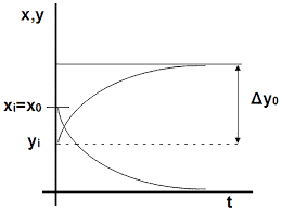
The maximum principle holds because if $u$ first crosses from positive to negative values at time $t_0$ at the point $x_0$, and if $u(x, t)$ has a nondegenerate minimum at $x_0$, then $u_{x x}\left(x_0, t_0\right)>0$. Hence, from $(1.5), u_t\left(x_0, t_0\right)>0$, so $u$ cannot evolve forward in time into the region $u<0$. A more careful argument is required to deal with degenerate minima, and with boundaries, but the conclusion is the same [18, 42]. A similar argument shows that $u(x, t) \leq 1$ for all $t \geq 0$ if $u_0(x) \leq 1$.

Remark 1.3. A forth-order diffusion equation, such as
$$
u_t=-u_{x x x x}+u(1-u)
$$
does not satisfy a maximum principle, and it is possible for positive initial data to evolve into negative values.

Spatially uniform solutions of (1.5) satisfy the logistic equation
(1.6) $u_t=k u(a-u)$.
This ODE has two equilibrium solutions at $u=0, u=a$.
The solution $u=0$ corresponds to a complete absence of the species, and is unstable. Small disturbances grow initially like $u_0 e^{k a t}$. The solution $u=a$ corresponds to the maximum population that can be sustained by the available resources. It is globally asymptotically stable, meaning that any solution of (1.6) with a strictly positive initial value approaches $a$ as $t \rightarrow \infty$.

Thus, the PDE (1.5) describes the evolution of a population that satisfies logistic dynamics at each point of space coupled with dispersal into regions of lower population.

数学代写|应用数学代写applied mathematics代考|Nondimensionalization

Before discussing (1.5) further, we simplify the equation by rescaling the variables to remove the constants. Let
$$
u=U \bar{u}, \quad x=L \bar{x}, \quad t=T \bar{t}
$$
where $U, L, T$ are arbitrary positive constants. Then
$$
\frac{\partial}{\partial x}=\frac{1}{L} \frac{\partial}{\partial \bar{x}}, \frac{\partial}{\partial t}=\frac{1}{T} \frac{\partial}{\partial \bar{t}} .
$$
It follows that $\bar{u}(\bar{x}, \bar{t})$ satisfies
$$
\bar{u}{\bar{t}}=\left(\frac{\nu T}{L^2}\right) \bar{u}{x x}+(k T U) \bar{u}\left(\frac{a}{U}-\bar{u}\right) .
$$
Therefore, choosing
$$
U=a, \quad T=\frac{1}{k a}, \quad L=\sqrt{\frac{\nu}{k a}},
$$
and dropping the bars, we find that $u(x, t)$ satisfies
(1.8) $u_t=u_{x x}+u(1-u)$.
Thus, in the absence of any other parameters, none of the coefficients in (1.5) are essential.

If we consider (1.5) on a finite domain of length $\ell$, then the problem depends in an essential way on a dimensionless constant $R$, which we may write as
$$
\mathrm{R}=\frac{k a \ell^2}{\nu} .
$$
We could equivalently use $1 / \mathrm{R}$ or $\sqrt{\mathrm{R}}$, or some other expression, instead of $\mathrm{R}$. From (1.7), we have $\mathrm{R}=T_d / T_r$ where $T_r=T$ is a timescale for solutions of the reaction equation (1.6) to approach the equilibrium value $a$, and $T_d=\ell^2 / \nu$ is a timescale for linear diffusion to significantly influence the entire length $\ell$ of the domain. The qualitative behavior of solutions depends on R.

数学代写|应用数学代写applied mathematics代考|MATH101

应用数学代考

数学代写|应用数学代写applied mathematics代考|Maximum principle

根据极大值原理,解 (1.5)如果初始数据保持非负 $u_0(x)=u(x, 0)$ 是非负的,这与其用作人口或概率模型是一 致的。
最大原则成立,因为如果 $u$ 首先从正值穿越到负值 $t_0$ 在这一点上 $x_0$ ,而如果 $u(x, t)$ 有一个非退化的最小值 $x_0$ , 然后 $u_{x x}\left(x_0, t_0\right)>0$. 因此,从 $(1.5), u_t\left(x_0, t_0\right)>0$ ,所以 $u$ 无法及时向前演化进入该区域 $u<0$. 需要更 仔细的论证来处理退化最小值和边界,但结论是相同的 $[18 , 42]$ 。类似的论证表明 $u(x, t) \leq 1$ 对所有人 $t \geq 0$ 如果 $u_0(x) \leq 1$.
备注 1.3。四阶扩散方程,例如
$$
u_t=-u_{x x x x}+u(1-u)
$$
不满足极大值原则,正初始数据有可能演化为负值。
(1.5) 的空间均匀解满足 logistic 方程
$$
\text { (1.6) } u_t=k u(a-u) \text {. }
$$
此 ODE 在处有两个平衡解 $u=0, u=a$.
解决方案 $u=0$ 对应于该物种的完全缺失,并且是不稳定的。小干扰最初会像 $u_0 e^{k a t}$. 解决方案 $u=a$ 对应于可 用资源可以维持的最大人口。它是全局渐近稳定的,这意味着 (1.6) 的任何具有严格正初始值的解都趋近 $a$ 作为 $t \rightarrow \infty$
因此,PDE (1.5) 描述了人口的演化,该人口在空间的每个点都满足逻辑动力学,并分散到人口较少的地区。

数学代写|应用数学代写applied mathematics代考|Nondimensionalization

在进一步讨论 (1.5) 之前,我们通过重新调整变量以移除常数来简化方程。让
$$
u=U \bar{u}, \quad x=L \bar{x}, \quad t=T \bar{t}
$$
在哪里 $U, L, T$ 是任意正常数。然后
$$
\frac{\partial}{\partial x}=\frac{1}{L} \frac{\partial}{\partial \bar{x}}, \frac{\partial}{\partial t}=\frac{1}{T} \frac{\partial}{\partial \bar{t}} .
$$
它遵循 $\bar{u}(\bar{x}, \bar{t})$ 满足
$$
\bar{u} \bar{t}=\left(\frac{\nu T}{L^2}\right) \bar{u} x x+(k T U) \bar{u}\left(\frac{a}{U}-\bar{u}\right)
$$
因此,选择
$$
U=a, \quad T=\frac{1}{k a}, \quad L=\sqrt{\frac{\nu}{k a}},
$$
放下酒吧,我们发现 $u(x, t)$ 满足
$$
(1.8) u_t=u_{x x}+u(1-u) \text {. }
$$
因此,在没有任何其他参数的情况下,(1.5) 中的系数都不是必需的。
$$
\mathrm{R}=\frac{k a \ell^2}{\nu} .
$$
我们可以等效地使用 $1 / \mathrm{R}$ 或者 $\sqrt{\mathrm{R}}$ ,或其他一些表达式,而不是 $\mathrm{R}$. 从 (1.7) 中,我们有 $\mathrm{R}=T_d / T_r$ 在哪里 $T_r=T$ 是反应方程式 (1.6) 的解接近平衡值的时间尺度 $a$ ,和 $T_d=\ell^2 / \nu$ 是线性扩散显着影响整个长度的时间 尺度 $\ell$ 域的。解决方案的定性行为取决于 $\mathrm{R}$ 。

数学代写|应用数学代写applied mathematics代考 请认准statistics-lab™

统计代写请认准statistics-lab™. statistics-lab™为您的留学生涯保驾护航。

金融工程代写

金融工程是使用数学技术来解决金融问题。金融工程使用计算机科学、统计学、经济学和应用数学领域的工具和知识来解决当前的金融问题,以及设计新的和创新的金融产品。

非参数统计代写

非参数统计指的是一种统计方法,其中不假设数据来自于由少数参数决定的规定模型;这种模型的例子包括正态分布模型和线性回归模型。

广义线性模型代考

广义线性模型(GLM)归属统计学领域,是一种应用灵活的线性回归模型。该模型允许因变量的偏差分布有除了正态分布之外的其它分布。

术语 广义线性模型(GLM)通常是指给定连续和/或分类预测因素的连续响应变量的常规线性回归模型。它包括多元线性回归,以及方差分析和方差分析(仅含固定效应)。

有限元方法代写

有限元方法(FEM)是一种流行的方法,用于数值解决工程和数学建模中出现的微分方程。典型的问题领域包括结构分析、传热、流体流动、质量运输和电磁势等传统领域。

有限元是一种通用的数值方法,用于解决两个或三个空间变量的偏微分方程(即一些边界值问题)。为了解决一个问题,有限元将一个大系统细分为更小、更简单的部分,称为有限元。这是通过在空间维度上的特定空间离散化来实现的,它是通过构建对象的网格来实现的:用于求解的数值域,它有有限数量的点。边界值问题的有限元方法表述最终导致一个代数方程组。该方法在域上对未知函数进行逼近。[1] 然后将模拟这些有限元的简单方程组合成一个更大的方程系统,以模拟整个问题。然后,有限元通过变化微积分使相关的误差函数最小化来逼近一个解决方案。

tatistics-lab作为专业的留学生服务机构,多年来已为美国、英国、加拿大、澳洲等留学热门地的学生提供专业的学术服务,包括但不限于Essay代写,Assignment代写,Dissertation代写,Report代写,小组作业代写,Proposal代写,Paper代写,Presentation代写,计算机作业代写,论文修改和润色,网课代做,exam代考等等。写作范围涵盖高中,本科,研究生等海外留学全阶段,辐射金融,经济学,会计学,审计学,管理学等全球99%专业科目。写作团队既有专业英语母语作者,也有海外名校硕博留学生,每位写作老师都拥有过硬的语言能力,专业的学科背景和学术写作经验。我们承诺100%原创,100%专业,100%准时,100%满意。

随机分析代写


随机微积分是数学的一个分支,对随机过程进行操作。它允许为随机过程的积分定义一个关于随机过程的一致的积分理论。这个领域是由日本数学家伊藤清在第二次世界大战期间创建并开始的。

时间序列分析代写

随机过程,是依赖于参数的一组随机变量的全体,参数通常是时间。 随机变量是随机现象的数量表现,其时间序列是一组按照时间发生先后顺序进行排列的数据点序列。通常一组时间序列的时间间隔为一恒定值(如1秒,5分钟,12小时,7天,1年),因此时间序列可以作为离散时间数据进行分析处理。研究时间序列数据的意义在于现实中,往往需要研究某个事物其随时间发展变化的规律。这就需要通过研究该事物过去发展的历史记录,以得到其自身发展的规律。

回归分析代写

多元回归分析渐进(Multiple Regression Analysis Asymptotics)属于计量经济学领域,主要是一种数学上的统计分析方法,可以分析复杂情况下各影响因素的数学关系,在自然科学、社会和经济学等多个领域内应用广泛。

MATLAB代写

MATLAB 是一种用于技术计算的高性能语言。它将计算、可视化和编程集成在一个易于使用的环境中,其中问题和解决方案以熟悉的数学符号表示。典型用途包括:数学和计算算法开发建模、仿真和原型制作数据分析、探索和可视化科学和工程图形应用程序开发,包括图形用户界面构建MATLAB 是一个交互式系统,其基本数据元素是一个不需要维度的数组。这使您可以解决许多技术计算问题,尤其是那些具有矩阵和向量公式的问题,而只需用 C 或 Fortran 等标量非交互式语言编写程序所需的时间的一小部分。MATLAB 名称代表矩阵实验室。MATLAB 最初的编写目的是提供对由 LINPACK 和 EISPACK 项目开发的矩阵软件的轻松访问,这两个项目共同代表了矩阵计算软件的最新技术。MATLAB 经过多年的发展,得到了许多用户的投入。在大学环境中,它是数学、工程和科学入门和高级课程的标准教学工具。在工业领域,MATLAB 是高效研究、开发和分析的首选工具。MATLAB 具有一系列称为工具箱的特定于应用程序的解决方案。对于大多数 MATLAB 用户来说非常重要,工具箱允许您学习应用专业技术。工具箱是 MATLAB 函数(M 文件)的综合集合,可扩展 MATLAB 环境以解决特定类别的问题。可用工具箱的领域包括信号处理、控制系统、神经网络、模糊逻辑、小波、仿真等。

R语言代写问卷设计与分析代写
PYTHON代写回归分析与线性模型代写
MATLAB代写方差分析与试验设计代写
STATA代写机器学习/统计学习代写
SPSS代写计量经济学代写
EVIEWS代写时间序列分析代写
EXCEL代写深度学习代写
SQL代写各种数据建模与可视化代写

数学代写|应用数学代写applied mathematics代考|Math2090

如果你也在 怎样代写应用数学applied mathematics这个学科遇到相关的难题,请随时右上角联系我们的24/7代写客服。

应用数学是不同领域对数学方法的应用,如物理学、工程学、医学、生物学、金融、商业、计算机科学和工业。

statistics-lab™ 为您的留学生涯保驾护航 在代写应用数学applied mathematics方面已经树立了自己的口碑, 保证靠谱, 高质且原创的统计Statistics代写服务。我们的专家在代写应用数学applied mathematics代写方面经验极为丰富,各种代写应用数学applied mathematics相关的作业也就用不着说。

我们提供的应用数学applied mathematics及其相关学科的代写,服务范围广, 其中包括但不限于:

  • Statistical Inference 统计推断
  • Statistical Computing 统计计算
  • Advanced Probability Theory 高等概率论
  • Advanced Mathematical Statistics 高等数理统计学
  • (Generalized) Linear Models 广义线性模型
  • Statistical Machine Learning 统计机器学习
  • Longitudinal Data Analysis 纵向数据分析
  • Foundations of Data Science 数据科学基础
数学代写|应用数学代写applied mathematics代考|Math2090

数学代写|应用数学代写applied mathematics代考|Constitutive equations

The conservation law (1.2) is not a closed equation for the density $u$. Typically, we supplement it with constitutive equations that relate the flux $\vec{q}$ and the source density $\sigma$ to $u$ and its derivatives. While the conservation law expresses a general physical principle, constitutive equations describe the response of a particular system being modeled.
Example 1.1. If the flux and source are pointwise functions of the density,
$$
\vec{q}=\vec{f}(u), \quad \sigma=g(u),
$$
then we get a first-order system of PDEs
$$
u_t+\nabla \cdot \vec{f}(u)=g(u) .
$$
For example, in one space dimension, if $g(u)=0$ and $f(u)=u^2 / 2$, we get the inviscid Burgers equation
$$
u_t+\left(\frac{1}{2} u^2\right)_x=0 .
$$
This equation is a basic model equation for hyperbolic systems of conservation laws, such as the compressible Euler equations for the flow of an inviscid compressible fluid [47].

Example 1.2. Suppose that the flux is a linear function of the density gradient,
$$
\vec{q}=-A \nabla u,
$$
where $A$ is a second-order tensor, that is a linear map between vectors. It is represented by an $n \times n$ matrix with respect to a choice of $n$ basis vectors. Then, if $\sigma=0$, we get a second order, linear PDE for $u(\vec{x}, t)$
$$
u_t=\nabla \cdot(A \nabla u) .
$$
Examples of this constitutive equation include: Fourier’s law in heat conduction (heat flux is a linear function of temperature gradient); Fick’s law (flux of solute is a linear function of the concentration gradient); and Darcy’s law (fluid velocity in a porous medium is a linear function of the pressure gradient). It is interesting to note how old each of these laws is: Fourier (1822); Fick (1855); Darcy (1855).
The conductivity tensor $A$ in (1.3) is usually symmetric and positive-definite, in which case (1.4) is a parabolic PDE; the corresponding PDE for equilibrium density distributions $u(\vec{x})$ is then an elliptic equation
$$
\nabla \cdot(A \nabla u)=0
$$

数学代写|应用数学代写applied mathematics代考|The KPP equation

If $\vec{q}=-\nu \nabla u$ and $\sigma=f(u)$ in (1.2), we get a reaction-diffusion equation
$$
u_l=\nu \Delta u+f(u) \text {. }
$$
Spatially uniform solutions satisfy the ODE
$$
u_t=f(u),
$$
which is the ‘reaction’ equation. In addition, diffusion couples together the solution at different points.

Such equations arise, for example, as models of spatially nonuniform chemical reactions, and of population dynamics in spatially distributed species.

The combined effects of spatial diffusion and nonlinear reaction can lead to the formation of many different types of spatial patterns; the spiral waves that occur in Belousov-Zabotinski reactions are one example.

One of the simplest reaction-diffusion equations is the KPP equation (or Fisher equation)
$u_t=\nu u_{x x}+k u(a-u)$
Here, $\nu, k, a$ are positive constants; as we will show, they may be set equal to 1 without loss of generality.

Equation (1.5) was introduced independently by Fisher [22], and Kolmogorov, Petrovsky, and Piskunov [33] in 1937. It provides a simple model for the dispersion of a spatially distributed species with population density $u(x, t)$ or, in Fisher’s work, for the advance of a favorable allele through a spatially distributed population.

数学代写|应用数学代写applied mathematics代考|Math2090

应用数学代考

数学代写|应用数学代写applied mathematics代考|Constitutive equations

守恒定律 (1.2) 不是密度的封闭方程 $u$. 通常,我们用与通量相关的本构方程来补充它 $q$ 和源密度 $\sigma$ 至 $u$ 及其衍生 物。守恒定律表达了一般的物理原理,而本构方程则描述了被建模的特定系统的响应。
示例 1.1。如果通量和源是密度的逐点函数,
$$
\vec{q}=\vec{f}(u), \quad \sigma=g(u),
$$
然后我们得到 PDE 的一阶系统
$$
u_t+\nabla \cdot \vec{f}(u)=g(u) .
$$
例如,在一个空间维度中,如果 $g(u)=0$ 和 $f(u)=u^2 / 2$, 我们得到无粘性的 Burgers 方程
$$
u_t+\left(\frac{1}{2} u^2\right)_x=0 .
$$
该方程是双曲线守恒定律系统的基本模型方程,例如无粘性可压缩流体流动的可压缩欧拉方程 [47]。
示例 1.2。假设通量是密度梯度的线性函数,
$$
\vec{q}=-A \nabla u
$$
在哪里 $A$ 是二阶张量,即向量之间的线性映射。它由一个代表 $n \times n$ 关于选择的矩阵 $n$ 基础向量。那么,如果 $\sigma=0$ ,我们得到二阶线性 PDE $u(\vec{x}, t)$
$$
u_t=\nabla \cdot(A \nabla u) .
$$
这种本构方程的例子包括:热传导中的傅立叶定律(热通量是温度梯度的线性函数);菲克定律 (溶质通量是 浓度梯度的线性函数);和达西定律(多孔介质中的流体速度是压力梯度的线性函数)。有趣的是注意这些定律 中的每一个有多古老: Fourier (1822);菲克 (1855 年);达西 (1855 年) 。
电导率张量 $A(1.3)$ 中的通常是对称且正定的,在这种情况下 (1.4) 是抛物线 PDE;平衡密度分布的相应 PDE $u(\vec{x})$ 则为椭圆方程
$$
\nabla \cdot(A \nabla u)=0
$$

数学代写|应用数学代写applied mathematics代考|The KPP equation

如果 $\vec{q}=-\nu \nabla u$ 和 $\sigma=f(u)$ 在(1.2)中,我们得到一个反应扩散方程
$$
u_l=\nu \Delta u+f(u) .
$$
空间均匀解满足 ODE
$$
u_t=f(u),
$$
这是“反应”方程。此外,扩散将不同点的溶液耦合在一起。
例如,此类方程作为空间非均匀化学反应模型和空间分布物种的种群动态模型出现。
空间扩散和非线性反应的综合作用可以导致形成许多不同类型的空间格局;Belousov-Zabotinski 反应中发生的 螺旋波就是一个例子。
最简单的反应扩散方程之一是 KPP 方程 (或 Fisher 方程)
$$
u_t=\nu u_{x x}+k u(a-u)
$$
这里, $\nu, k, a$ 是正常数;正如我们将要展示的,在不失一般性的情况下,它们可以设置为等于 1 。
方程 (1.5) 由 Fisher [22] 和 Kolmogorov、Petrovsky 和 Piskunov [33] 于 1937 年独立引入。它为具有种群密 度的空间分布物种的扩散提供了一个简单的模型 $u(x, t)$ 或者,在 Fisher 的工作中,通过空间分布的种群推进有 利的等位基因。

数学代写|应用数学代写applied mathematics代考 请认准statistics-lab™

统计代写请认准statistics-lab™. statistics-lab™为您的留学生涯保驾护航。

金融工程代写

金融工程是使用数学技术来解决金融问题。金融工程使用计算机科学、统计学、经济学和应用数学领域的工具和知识来解决当前的金融问题,以及设计新的和创新的金融产品。

非参数统计代写

非参数统计指的是一种统计方法,其中不假设数据来自于由少数参数决定的规定模型;这种模型的例子包括正态分布模型和线性回归模型。

广义线性模型代考

广义线性模型(GLM)归属统计学领域,是一种应用灵活的线性回归模型。该模型允许因变量的偏差分布有除了正态分布之外的其它分布。

术语 广义线性模型(GLM)通常是指给定连续和/或分类预测因素的连续响应变量的常规线性回归模型。它包括多元线性回归,以及方差分析和方差分析(仅含固定效应)。

有限元方法代写

有限元方法(FEM)是一种流行的方法,用于数值解决工程和数学建模中出现的微分方程。典型的问题领域包括结构分析、传热、流体流动、质量运输和电磁势等传统领域。

有限元是一种通用的数值方法,用于解决两个或三个空间变量的偏微分方程(即一些边界值问题)。为了解决一个问题,有限元将一个大系统细分为更小、更简单的部分,称为有限元。这是通过在空间维度上的特定空间离散化来实现的,它是通过构建对象的网格来实现的:用于求解的数值域,它有有限数量的点。边界值问题的有限元方法表述最终导致一个代数方程组。该方法在域上对未知函数进行逼近。[1] 然后将模拟这些有限元的简单方程组合成一个更大的方程系统,以模拟整个问题。然后,有限元通过变化微积分使相关的误差函数最小化来逼近一个解决方案。

tatistics-lab作为专业的留学生服务机构,多年来已为美国、英国、加拿大、澳洲等留学热门地的学生提供专业的学术服务,包括但不限于Essay代写,Assignment代写,Dissertation代写,Report代写,小组作业代写,Proposal代写,Paper代写,Presentation代写,计算机作业代写,论文修改和润色,网课代做,exam代考等等。写作范围涵盖高中,本科,研究生等海外留学全阶段,辐射金融,经济学,会计学,审计学,管理学等全球99%专业科目。写作团队既有专业英语母语作者,也有海外名校硕博留学生,每位写作老师都拥有过硬的语言能力,专业的学科背景和学术写作经验。我们承诺100%原创,100%专业,100%准时,100%满意。

随机分析代写


随机微积分是数学的一个分支,对随机过程进行操作。它允许为随机过程的积分定义一个关于随机过程的一致的积分理论。这个领域是由日本数学家伊藤清在第二次世界大战期间创建并开始的。

时间序列分析代写

随机过程,是依赖于参数的一组随机变量的全体,参数通常是时间。 随机变量是随机现象的数量表现,其时间序列是一组按照时间发生先后顺序进行排列的数据点序列。通常一组时间序列的时间间隔为一恒定值(如1秒,5分钟,12小时,7天,1年),因此时间序列可以作为离散时间数据进行分析处理。研究时间序列数据的意义在于现实中,往往需要研究某个事物其随时间发展变化的规律。这就需要通过研究该事物过去发展的历史记录,以得到其自身发展的规律。

回归分析代写

多元回归分析渐进(Multiple Regression Analysis Asymptotics)属于计量经济学领域,主要是一种数学上的统计分析方法,可以分析复杂情况下各影响因素的数学关系,在自然科学、社会和经济学等多个领域内应用广泛。

MATLAB代写

MATLAB 是一种用于技术计算的高性能语言。它将计算、可视化和编程集成在一个易于使用的环境中,其中问题和解决方案以熟悉的数学符号表示。典型用途包括:数学和计算算法开发建模、仿真和原型制作数据分析、探索和可视化科学和工程图形应用程序开发,包括图形用户界面构建MATLAB 是一个交互式系统,其基本数据元素是一个不需要维度的数组。这使您可以解决许多技术计算问题,尤其是那些具有矩阵和向量公式的问题,而只需用 C 或 Fortran 等标量非交互式语言编写程序所需的时间的一小部分。MATLAB 名称代表矩阵实验室。MATLAB 最初的编写目的是提供对由 LINPACK 和 EISPACK 项目开发的矩阵软件的轻松访问,这两个项目共同代表了矩阵计算软件的最新技术。MATLAB 经过多年的发展,得到了许多用户的投入。在大学环境中,它是数学、工程和科学入门和高级课程的标准教学工具。在工业领域,MATLAB 是高效研究、开发和分析的首选工具。MATLAB 具有一系列称为工具箱的特定于应用程序的解决方案。对于大多数 MATLAB 用户来说非常重要,工具箱允许您学习应用专业技术。工具箱是 MATLAB 函数(M 文件)的综合集合,可扩展 MATLAB 环境以解决特定类别的问题。可用工具箱的领域包括信号处理、控制系统、神经网络、模糊逻辑、小波、仿真等。

R语言代写问卷设计与分析代写
PYTHON代写回归分析与线性模型代写
MATLAB代写方差分析与试验设计代写
STATA代写机器学习/统计学习代写
SPSS代写计量经济学代写
EVIEWS代写时间序列分析代写
EXCEL代写深度学习代写
SQL代写各种数据建模与可视化代写

数学代写|伽罗瓦理论代写Galois Theory代考|МАТН3040

如果你也在 怎样代写伽罗瓦理论Galois Theory这个学科遇到相关的难题,请随时右上角联系我们的24/7代写客服。

伽罗瓦理论的中心思想是考虑根的排列(或重新排列),使根所满足的任何代数方程在根被排列后仍然满足。最初,该理论是针对系数为有理数的代数方程而开发的。

statistics-lab™ 为您的留学生涯保驾护航 在代写伽罗瓦理论Galois Theory方面已经树立了自己的口碑, 保证靠谱, 高质且原创的统计Statistics代写服务。我们的专家在代写伽罗瓦理论Galois Theory代写方面经验极为丰富,各种代写伽罗瓦理论Galois Theory相关的作业也就用不着说。

我们提供的伽罗瓦理论Galois Theory及其相关学科的代写,服务范围广, 其中包括但不限于:

  • Statistical Inference 统计推断
  • Statistical Computing 统计计算
  • Advanced Probability Theory 高等概率论
  • Advanced Mathematical Statistics 高等数理统计学
  • (Generalized) Linear Models 广义线性模型
  • Statistical Machine Learning 统计机器学习
  • Longitudinal Data Analysis 纵向数据分析
  • Foundations of Data Science 数据科学基础
数学代写|伽罗瓦理论代写Galois Theory代考|МАТН3040

数学代写|伽罗瓦理论代写Galois Theory代考|Quintic Equations

So far, we have a series of special tricks, different in each case. We can approach the general quintic equation
$$
t^5+a t^4+b t^3+c t^2+d t+e=0
$$
in a similar way. A Tschirnhaus transformation $y=t+a / 5$ reduces it to
$$
y^5+p y^3+q y^2+r y+s=0
$$
However, all variations on the tricks that we used for the quadratic, cubic, and quartic equations grind to a halt.

In 1770-1771 Lagrange analysed all of the above special tricks, showing that they can all be ‘explained’ using general principles about symmetric functions of the roots. When he applied this method to the quintic, however, he found that it ‘reduced’ the problem to a sextic – an equation of degree 6. Instead of helping, the method made the problem worse.

Lagrange observed that all methods for solving polynomial equations by radicals involve constructing rational functions of the roots that take a small number of values when the roots $\alpha_j$ are permuted. Prominent among these is the expression
$$
\delta=\prod_{1 \leq j<k \leq n}\left(\alpha_j-\alpha_k\right)
$$
where $n$ is the degree. This takes just two values, $\pm \delta$ : plus for even permutations and minus for odd ones. Therefore $\Delta=\delta^2$ (known as the discriminant because it is nonzero precisely when the roots are distinct, so it ‘discriminates’ among the roots) is a rational function of the coefficients. This gets us started, and it yields a complete solution for the quadratic, but for cubics upwards it does not help much unless we can find other expressions in the roots with similar properties under permutation.

Lagrange worked out what these expressions look like for the cubic and the quartic, and noticed a pattern. For example, if a cubic polynomial has roots $\alpha_1, \alpha_2, \alpha_3$, and $\omega$ is a primitive cube root of unity, then the expression
$$
u=\left(\alpha_1+\omega \alpha_2+\omega^2 \alpha_3\right)^3
$$ takes exactly two distinct values.

数学代写|伽罗瓦理论代写Galois Theory代考|The Fundamental Theorem of Algebra

At the time of Galois, the natural setting for most mathematical investigations was the complex number system. The real numbers were inadequate for many questions, because $-1$ has no real square root. The arithmetic, algebra, anddecisively – analysis of complex numbers were richer, more elegant, and more complete than the corresponding theories for real numbers.

In this chapter we establish one of the key properties of $\mathbb{C}$, known as the Fundamental Theorem of Algebra. This theorem asserts that every polynomial equation with coefficients in $\mathbb{C}$ has a solution in $\mathbb{C}$. This theorem is, of course, false over $\mathbb{R}$-consider the equation $t^2+1=0$. It was fundamental to classical algebra, but the name is somewhat archaic, and modern algebra bypasses $\mathbb{C}$ altogether, preferring greater generality. Because we find it convenient to work in the same setting as Galois, the theorem is fundamental for us.

All rigorous proofs of the Fundamental Theorem of Algebra require quite a lot of background. Here, we give a proof that uses a few simple ideas from algebra and trigonometry, estimates of the kind that are familiar from any first course in analysis, and one simple basic result from point-set topology. Later, we give an almost purely algebraic proof, but the price is the need for much more machinery: see Chapter 23. Ironically, that proof uses Galois theory to prove the Fundamental Theorem of Algebra, the exact opposite of what Galois did. The logic is not circular, because the proof in Chapter 23 rests on the abstract approach to Galois theory described in the second part of this book, which makes no use of the Fundamental Theorem of Algebra.

数学代写|伽罗瓦理论代写Galois Theory代考|МАТН3040

伽罗瓦理论代考

数学代写|伽罗瓦理论代写Galois Theory代考|Quintic Equations

到目前为止,我们有一系列特殊技巧,每种情况都不同。我们可以接近一般的五次方程
$$
t^5+a t^4+b t^3+c t^2+d t+e=0
$$
以类似的方式。Tschirnhaus 变换 $y=t+a / 5$ 减少到
$$
y^5+p y^3+q y^2+r y+s=0
$$
然而,我们用于二次、三次和四次方程式的技巧的所有变体都停止了。
在 1770-1771 年,拉格朗日分析了上述所有特殊技巧,表明它们都可以使用关于根的对称函数的一般原理来“解 释”。然而,当他将这种方法应用于五次方程时,他发现它将问题“简化”为六次方程一一一个 6 次方程。该方法 非但没有帮助,反而使问题变得更糟。
拉格朗日观察到,所有用根求解多项式方程的方法都涉及构造根的有理函数,这些函数在根时取少量值 $\alpha_j$ 被置 换。其中突出的是表达
$$
\delta=\prod_{1 \leq j<k \leq n}\left(\alpha_j-\alpha_k\right)
$$
在哪里 $n$ 是学位。这只需要两个值, $\pm \delta$ : 偶数排列加号,奇数排列减号。所以 $\Delta=\delta^2$ (称为判别式,因为它恰 好在根不同时不为零,因此它在根中 “区分”) 是系数的有理函数。这让我们开始了,它为二次方程产生了一个完 整的解,但对于向上的三次方程它并没有太大帮助,除非我们可以在根中找到其他具有类似排列性质的表达式。
拉格朗日计算出了这些表达式对于三次和四次的样子,并注意到了一种模式。例如,如果三次多项式有根 $\alpha_1, \alpha_2, \alpha_3$ ,和 $\omega$ 是单位的原始立方根,则表达式
$$
u=\left(\alpha_1+\omega \alpha_2+\omega^2 \alpha_3\right)^3
$$
恰好采用两个不同的值。

数学代写|伽罗瓦理论代写Galois Theory代考|The Fundamental Theorem of Algebra

在伽罗瓦时代,大多数数学研究的自然背景是复数系统。许多问题的真实数字是不够的,因为−1没有真正的平方根。算术、代数和决定性的复数分析比相应的实数理论更丰富、更优雅、更完整。

在本章中,我们建立了一个关键属性C,被称为代数基本定理。该定理断言每个系数为C有一个解决方案C. 这个定理当然是错误的R-考虑方程吨2+1=0. 它是经典代数的基础,但这个名字有点陈旧,现代代数绕过了C总的来说,更喜欢更大的普遍性。因为我们发现在与 Galois 相同的环境中工作很方便,所以该定理是我们的基础。

代数基本定理的所有严格证明都需要相当多的背景知识。在这里,我们给出了一个证明,其中使用了代数和三角学中的一些简单思想、任何第一门分析课程中熟悉的那种估计,以及点集拓扑的一个简单基本结果。稍后,我们给出了一个几乎纯代数的证明,但代价是需要更多的机器:见第 23 章。具有讽刺意味的是,该证明使用伽罗瓦理论来证明代数基本定理,与伽罗瓦所做的完全相反。逻辑不是循环的,因为第 23 章中的证明基于本书第二部分描述的伽罗瓦理论的抽象方法,它没有使用代数基本定理。

数学代写|伽罗瓦理论代写Galois Theory代考 请认准statistics-lab™

统计代写请认准statistics-lab™. statistics-lab™为您的留学生涯保驾护航。

金融工程代写

金融工程是使用数学技术来解决金融问题。金融工程使用计算机科学、统计学、经济学和应用数学领域的工具和知识来解决当前的金融问题,以及设计新的和创新的金融产品。

非参数统计代写

非参数统计指的是一种统计方法,其中不假设数据来自于由少数参数决定的规定模型;这种模型的例子包括正态分布模型和线性回归模型。

广义线性模型代考

广义线性模型(GLM)归属统计学领域,是一种应用灵活的线性回归模型。该模型允许因变量的偏差分布有除了正态分布之外的其它分布。

术语 广义线性模型(GLM)通常是指给定连续和/或分类预测因素的连续响应变量的常规线性回归模型。它包括多元线性回归,以及方差分析和方差分析(仅含固定效应)。

有限元方法代写

有限元方法(FEM)是一种流行的方法,用于数值解决工程和数学建模中出现的微分方程。典型的问题领域包括结构分析、传热、流体流动、质量运输和电磁势等传统领域。

有限元是一种通用的数值方法,用于解决两个或三个空间变量的偏微分方程(即一些边界值问题)。为了解决一个问题,有限元将一个大系统细分为更小、更简单的部分,称为有限元。这是通过在空间维度上的特定空间离散化来实现的,它是通过构建对象的网格来实现的:用于求解的数值域,它有有限数量的点。边界值问题的有限元方法表述最终导致一个代数方程组。该方法在域上对未知函数进行逼近。[1] 然后将模拟这些有限元的简单方程组合成一个更大的方程系统,以模拟整个问题。然后,有限元通过变化微积分使相关的误差函数最小化来逼近一个解决方案。

tatistics-lab作为专业的留学生服务机构,多年来已为美国、英国、加拿大、澳洲等留学热门地的学生提供专业的学术服务,包括但不限于Essay代写,Assignment代写,Dissertation代写,Report代写,小组作业代写,Proposal代写,Paper代写,Presentation代写,计算机作业代写,论文修改和润色,网课代做,exam代考等等。写作范围涵盖高中,本科,研究生等海外留学全阶段,辐射金融,经济学,会计学,审计学,管理学等全球99%专业科目。写作团队既有专业英语母语作者,也有海外名校硕博留学生,每位写作老师都拥有过硬的语言能力,专业的学科背景和学术写作经验。我们承诺100%原创,100%专业,100%准时,100%满意。

随机分析代写


随机微积分是数学的一个分支,对随机过程进行操作。它允许为随机过程的积分定义一个关于随机过程的一致的积分理论。这个领域是由日本数学家伊藤清在第二次世界大战期间创建并开始的。

时间序列分析代写

随机过程,是依赖于参数的一组随机变量的全体,参数通常是时间。 随机变量是随机现象的数量表现,其时间序列是一组按照时间发生先后顺序进行排列的数据点序列。通常一组时间序列的时间间隔为一恒定值(如1秒,5分钟,12小时,7天,1年),因此时间序列可以作为离散时间数据进行分析处理。研究时间序列数据的意义在于现实中,往往需要研究某个事物其随时间发展变化的规律。这就需要通过研究该事物过去发展的历史记录,以得到其自身发展的规律。

回归分析代写

多元回归分析渐进(Multiple Regression Analysis Asymptotics)属于计量经济学领域,主要是一种数学上的统计分析方法,可以分析复杂情况下各影响因素的数学关系,在自然科学、社会和经济学等多个领域内应用广泛。

MATLAB代写

MATLAB 是一种用于技术计算的高性能语言。它将计算、可视化和编程集成在一个易于使用的环境中,其中问题和解决方案以熟悉的数学符号表示。典型用途包括:数学和计算算法开发建模、仿真和原型制作数据分析、探索和可视化科学和工程图形应用程序开发,包括图形用户界面构建MATLAB 是一个交互式系统,其基本数据元素是一个不需要维度的数组。这使您可以解决许多技术计算问题,尤其是那些具有矩阵和向量公式的问题,而只需用 C 或 Fortran 等标量非交互式语言编写程序所需的时间的一小部分。MATLAB 名称代表矩阵实验室。MATLAB 最初的编写目的是提供对由 LINPACK 和 EISPACK 项目开发的矩阵软件的轻松访问,这两个项目共同代表了矩阵计算软件的最新技术。MATLAB 经过多年的发展,得到了许多用户的投入。在大学环境中,它是数学、工程和科学入门和高级课程的标准教学工具。在工业领域,MATLAB 是高效研究、开发和分析的首选工具。MATLAB 具有一系列称为工具箱的特定于应用程序的解决方案。对于大多数 MATLAB 用户来说非常重要,工具箱允许您学习应用专业技术。工具箱是 MATLAB 函数(M 文件)的综合集合,可扩展 MATLAB 环境以解决特定类别的问题。可用工具箱的领域包括信号处理、控制系统、神经网络、模糊逻辑、小波、仿真等。

R语言代写问卷设计与分析代写
PYTHON代写回归分析与线性模型代写
MATLAB代写方差分析与试验设计代写
STATA代写机器学习/统计学习代写
SPSS代写计量经济学代写
EVIEWS代写时间序列分析代写
EXCEL代写深度学习代写
SQL代写各种数据建模与可视化代写

数学代写|伽罗瓦理论代写Galois Theory代考|МАТH0701

如果你也在 怎样代写伽罗瓦理论Galois Theory这个学科遇到相关的难题,请随时右上角联系我们的24/7代写客服。

伽罗瓦理论的中心思想是考虑根的排列(或重新排列),使根所满足的任何代数方程在根被排列后仍然满足。最初,该理论是针对系数为有理数的代数方程而开发的。

statistics-lab™ 为您的留学生涯保驾护航 在代写伽罗瓦理论Galois Theory方面已经树立了自己的口碑, 保证靠谱, 高质且原创的统计Statistics代写服务。我们的专家在代写伽罗瓦理论Galois Theory代写方面经验极为丰富,各种代写伽罗瓦理论Galois Theory相关的作业也就用不着说。

我们提供的伽罗瓦理论Galois Theory及其相关学科的代写,服务范围广, 其中包括但不限于:

  • Statistical Inference 统计推断
  • Statistical Computing 统计计算
  • Advanced Probability Theory 高等概率论
  • Advanced Mathematical Statistics 高等数理统计学
  • (Generalized) Linear Models 广义线性模型
  • Statistical Machine Learning 统计机器学习
  • Longitudinal Data Analysis 纵向数据分析
  • Foundations of Data Science 数据科学基础
数学代写|伽罗瓦理论代写Galois Theory代考|МАТH0701

数学代写|伽罗瓦理论代写Galois Theory代考|Solving Equations

We tend to think of the great problems of mathematics as being things like Fermat’s Last Theorem, the Poincaré Conjecture, or the Riemann Hypothesis: problems of central importance that remained unsolved for decades or even centuries. But the really big problems of mathematics are more general. A problem that runs like an ancient river through the middle of the territory we are going to explore is: Find out how to solve equations. Or, as often as not, prove that it cannot be done with specified methods. What sort of equations? There are many kinds: Diophantine equations, differential equations (ordinary, partial, or delay), difference equations, integral equations, operator equations … For Galois, it was polynomial equations. We work up to those in easy stages.

Historically, new kinds of number like $\sqrt{2}$ or i were introduced because the old ones were inadequate for solving some important problems. Most such problems can be formulated using equations, though it must be said that this is a modern interpretation, and the ancient mathematicians did not think in quite those terms.

For example, the step from $\mathbb{N}$ to $\mathbb{Z}$ is needed because although some equations, such as
$$
t+2=7
$$
can be solved for $t \in \mathbb{N}$, others, such as
$$
t+7=2
$$
cannot. However, such equations can be solved in $\mathbb{Z}$, where $t=-5$ makes sense. (The symbol $x$ is more traditional than $t$ here, but it is convenient to standardise on $t$ for the rest of the book, so we may as well start straight away.)

Similarly, the step from $\mathbb{Z}$ to $\mathbb{Q}$ (historically, it was initially from $\mathbb{N}$ to $\mathbb{Q}^{+}$, the positive rationals) makes it possible to solve the equation
$$
2 t=7
$$
because $t=\frac{7}{2}$ makes sense in $\mathbb{Q}$.

数学代写|伽罗瓦理论代写Galois Theory代考|Peculiarities of Cardano’s Formula

An old warning, which goes back to Aesop’s Fables, is: ‘Be careful what you wish for: you might get it’. We have wished for a formula for the solution, and we have got one. It has its peculiarities.

First: recall that over $\mathbb{C}$, every nonzero complex number $z$ has three cube roots. If one of them is $\alpha$, then the other two are $\omega \alpha$ and $\omega^2 \alpha$, where
$$
\omega=-\frac{1}{2}+i \frac{\sqrt{3}}{2}
$$
is a primitive cube root of 1 . Then
$$
\omega^2=-\frac{1}{2}-\mathrm{i} \frac{\sqrt{3}}{2}
$$
The expression for $y$ therefore appears to lead to nine solutions of the form
$$
\begin{array}{lcr}
\alpha+\beta & \alpha+\omega \beta & \alpha+\omega^2 \beta \
\omega \alpha+\beta & \omega \alpha+\omega \beta & \omega \alpha+\omega^2 \beta \
\omega^2 \alpha+\beta & \omega^2 \alpha+\omega \beta & \omega^2 \alpha+\omega^2 \beta
\end{array}
$$
where $\alpha, \beta$ are specific choices of the cube roots.
However, not all of these expressions are zeros. Equation (1.5) implies (1.7), but (1.7) implies (1.5) only when we make the correct choices of cube roots. If we choose $\alpha, \beta$ so that $3 \alpha \beta+p=0$, then the solutions are
$$
\alpha+\beta \quad \omega \alpha+\omega^2 \beta \quad \omega^2 \alpha+\omega \beta
$$
Another peculiarity emerges when we try to solve equations whose solutions we already know. For example,
$$
y^3+3 y-36=0
$$

数学代写|伽罗瓦理论代写Galois Theory代考|МАТH0701

伽罗瓦理论代考

数学代写|伽罗瓦理论代写Galois Theory代考|Solving Equations

我们倾向于将数学中的重大问题视为诸如费马大定理、庞加莱猜想或黎曼猜想之类的问题: 几十年甚至几个世纪 以来仍末解决的核心问题。但真正大的数学问题是更普遍的。一个像古河一样流经我们将要探索的领土中间的问 题是: 找出如何求解方程。或者,通常情况下,证明它不能用指定的方法来完成。什么样的方程式? 有很多种: 丟番图方程、微分方程 (常微分方程、偏微分方程或延迟微分方程) 、差分方程、积分方程、算子方程……对于 伽罗瓦来说,就是多项式方程。我们努力达到那些简单的阶段。
从历史上看,新的数字类型如 $\sqrt{2}$ 或者我被介绍是因为旧的不足以解决一些重要的问题。大多数此类问题都可以 用方程式来表述,尽管必须说这是一种现代解释,而古代数学家并没有完全按照这些术语来思考。
例如,从 $\mathbb{N}$ 至 $\mathbb{Z}$ 是需要的,因为虽然有些方程式,例如
$$
t+2=7
$$
可以解决 $t \in \mathbb{N}$ ,其他的,比如
$$
t+7=2
$$
不能。然而,这样的方程式可以求解 $\mathbb{Z}$ , 在哪里 $t=-5$ 说得通。(符号 $x$ 比传统的 $t$ 在这里,但标准化很方便 $t$ 对于本书的其余部分,我们不妨直接开始。)
同样,从 $\mathbb{Z}$ 至 $\mathbb{Q}$ (从历史上看,它最初来自 $\mathbb{N}$ 至 $\mathbb{Q}^{+}$,正有理数) 使得求解方程成为可能
$$
2 t=7
$$
因为 $t=\frac{7}{2}$ 有道理 $\mathbb{Q}$.

数学代写|伽罗瓦理论代写Galois Theory代考|Peculiarities of Cardano’s Formula

一个古老的警告可以追溯到伊索寓言,它是: “小心你想要的东西:你可能会得到它”。我们希望有一个解决方案 的公式,我们已经有了。它有它的特点。
第一: 回想一下 $\mathbb{C}$ ,每个非零复数 $z$ 有三个立方根。如果其中之一是 $\alpha$ ,那么另外两个是 $\omega \alpha$ 和 $\omega^2 \alpha$ ,在哪里
$$
\omega=-\frac{1}{2}+i \frac{\sqrt{3}}{2}
$$
是 1 的原始立方根。然后
$$
\omega^2=-\frac{1}{2}-\mathrm{i} \frac{\sqrt{3}}{2}
$$
表达式为 $y$ 因此似乎导致九种形式的解决方案
$$
\alpha+\beta \quad \alpha+\omega \beta \quad \alpha+\omega^2 \beta \omega \alpha+\beta \quad \omega \alpha+\omega \beta \quad \omega \alpha+\omega^2 \beta \omega^2 \alpha+\beta \quad \omega^2 \alpha+\omega \beta \quad \omega^2 \alpha+\omega^2 \beta
$$
在哪里 $\alpha, \beta$ 是立方根的具体选择。
但是,并非所有这些表达式都是零。等式 (1.5) 蕴含 (1.7),但只有当我们正确选择立方根时,(1.7) 才蕴含 (1.5)。如果我们选择 $\alpha, \beta$ 以便 $3 \alpha \beta+p=0$ ,那么解是
$$
\alpha+\beta \quad \omega \alpha+\omega^2 \beta \quad \omega^2 \alpha+\omega \beta
$$
当我们尝试求解已知解的方程时,另一个特点就会出现。例如,
$$
y^3+3 y-36=0
$$

数学代写|伽罗瓦理论代写Galois Theory代考 请认准statistics-lab™

统计代写请认准statistics-lab™. statistics-lab™为您的留学生涯保驾护航。

金融工程代写

金融工程是使用数学技术来解决金融问题。金融工程使用计算机科学、统计学、经济学和应用数学领域的工具和知识来解决当前的金融问题,以及设计新的和创新的金融产品。

非参数统计代写

非参数统计指的是一种统计方法,其中不假设数据来自于由少数参数决定的规定模型;这种模型的例子包括正态分布模型和线性回归模型。

广义线性模型代考

广义线性模型(GLM)归属统计学领域,是一种应用灵活的线性回归模型。该模型允许因变量的偏差分布有除了正态分布之外的其它分布。

术语 广义线性模型(GLM)通常是指给定连续和/或分类预测因素的连续响应变量的常规线性回归模型。它包括多元线性回归,以及方差分析和方差分析(仅含固定效应)。

有限元方法代写

有限元方法(FEM)是一种流行的方法,用于数值解决工程和数学建模中出现的微分方程。典型的问题领域包括结构分析、传热、流体流动、质量运输和电磁势等传统领域。

有限元是一种通用的数值方法,用于解决两个或三个空间变量的偏微分方程(即一些边界值问题)。为了解决一个问题,有限元将一个大系统细分为更小、更简单的部分,称为有限元。这是通过在空间维度上的特定空间离散化来实现的,它是通过构建对象的网格来实现的:用于求解的数值域,它有有限数量的点。边界值问题的有限元方法表述最终导致一个代数方程组。该方法在域上对未知函数进行逼近。[1] 然后将模拟这些有限元的简单方程组合成一个更大的方程系统,以模拟整个问题。然后,有限元通过变化微积分使相关的误差函数最小化来逼近一个解决方案。

tatistics-lab作为专业的留学生服务机构,多年来已为美国、英国、加拿大、澳洲等留学热门地的学生提供专业的学术服务,包括但不限于Essay代写,Assignment代写,Dissertation代写,Report代写,小组作业代写,Proposal代写,Paper代写,Presentation代写,计算机作业代写,论文修改和润色,网课代做,exam代考等等。写作范围涵盖高中,本科,研究生等海外留学全阶段,辐射金融,经济学,会计学,审计学,管理学等全球99%专业科目。写作团队既有专业英语母语作者,也有海外名校硕博留学生,每位写作老师都拥有过硬的语言能力,专业的学科背景和学术写作经验。我们承诺100%原创,100%专业,100%准时,100%满意。

随机分析代写


随机微积分是数学的一个分支,对随机过程进行操作。它允许为随机过程的积分定义一个关于随机过程的一致的积分理论。这个领域是由日本数学家伊藤清在第二次世界大战期间创建并开始的。

时间序列分析代写

随机过程,是依赖于参数的一组随机变量的全体,参数通常是时间。 随机变量是随机现象的数量表现,其时间序列是一组按照时间发生先后顺序进行排列的数据点序列。通常一组时间序列的时间间隔为一恒定值(如1秒,5分钟,12小时,7天,1年),因此时间序列可以作为离散时间数据进行分析处理。研究时间序列数据的意义在于现实中,往往需要研究某个事物其随时间发展变化的规律。这就需要通过研究该事物过去发展的历史记录,以得到其自身发展的规律。

回归分析代写

多元回归分析渐进(Multiple Regression Analysis Asymptotics)属于计量经济学领域,主要是一种数学上的统计分析方法,可以分析复杂情况下各影响因素的数学关系,在自然科学、社会和经济学等多个领域内应用广泛。

MATLAB代写

MATLAB 是一种用于技术计算的高性能语言。它将计算、可视化和编程集成在一个易于使用的环境中,其中问题和解决方案以熟悉的数学符号表示。典型用途包括:数学和计算算法开发建模、仿真和原型制作数据分析、探索和可视化科学和工程图形应用程序开发,包括图形用户界面构建MATLAB 是一个交互式系统,其基本数据元素是一个不需要维度的数组。这使您可以解决许多技术计算问题,尤其是那些具有矩阵和向量公式的问题,而只需用 C 或 Fortran 等标量非交互式语言编写程序所需的时间的一小部分。MATLAB 名称代表矩阵实验室。MATLAB 最初的编写目的是提供对由 LINPACK 和 EISPACK 项目开发的矩阵软件的轻松访问,这两个项目共同代表了矩阵计算软件的最新技术。MATLAB 经过多年的发展,得到了许多用户的投入。在大学环境中,它是数学、工程和科学入门和高级课程的标准教学工具。在工业领域,MATLAB 是高效研究、开发和分析的首选工具。MATLAB 具有一系列称为工具箱的特定于应用程序的解决方案。对于大多数 MATLAB 用户来说非常重要,工具箱允许您学习应用专业技术。工具箱是 MATLAB 函数(M 文件)的综合集合,可扩展 MATLAB 环境以解决特定类别的问题。可用工具箱的领域包括信号处理、控制系统、神经网络、模糊逻辑、小波、仿真等。

R语言代写问卷设计与分析代写
PYTHON代写回归分析与线性模型代写
MATLAB代写方差分析与试验设计代写
STATA代写机器学习/统计学习代写
SPSS代写计量经济学代写
EVIEWS代写时间序列分析代写
EXCEL代写深度学习代写
SQL代写各种数据建模与可视化代写

数学代写|伽罗瓦理论代写Galois Theory代考|MX4082

如果你也在 怎样代写伽罗瓦理论Galois Theory这个学科遇到相关的难题,请随时右上角联系我们的24/7代写客服。

伽罗瓦理论的中心思想是考虑根的排列(或重新排列),使根所满足的任何代数方程在根被排列后仍然满足。最初,该理论是针对系数为有理数的代数方程而开发的。

statistics-lab™ 为您的留学生涯保驾护航 在代写伽罗瓦理论Galois Theory方面已经树立了自己的口碑, 保证靠谱, 高质且原创的统计Statistics代写服务。我们的专家在代写伽罗瓦理论Galois Theory代写方面经验极为丰富,各种代写伽罗瓦理论Galois Theory相关的作业也就用不着说。

我们提供的伽罗瓦理论Galois Theory及其相关学科的代写,服务范围广, 其中包括但不限于:

  • Statistical Inference 统计推断
  • Statistical Computing 统计计算
  • Advanced Probability Theory 高等概率论
  • Advanced Mathematical Statistics 高等数理统计学
  • (Generalized) Linear Models 广义线性模型
  • Statistical Machine Learning 统计机器学习
  • Longitudinal Data Analysis 纵向数据分析
  • Foundations of Data Science 数据科学基础
数学代写|伽罗瓦理论代写Galois Theory代考|MX4082

数学代写|伽罗瓦理论代写Galois Theory代考|Complex Numbers

A complex number has the form
$$
z=x+\mathrm{i} y
$$
where $x, y$ are real numbers and $\mathrm{i}^2=-1$. Therefore $\mathrm{i}=\sqrt{-1}$, in some sense.
Throughout, we use the Roman letter $\mathrm{i}$ for $\sqrt{-1}$. This frees up italic $i$ for other uses.

The easiest way to define what we mean by $\sqrt{-1}$ is to consider $\mathbb{C}$ as the set $\mathbb{R}^2$ of all pairs of real numbers $(x, y)$, with algebraic operations
$$
\begin{aligned}
\left(x_1, y_1\right)+\left(x_2, y_2\right) &=\left(x_1+x_2, y_1+y_2\right) \
\left(x_1, y_1\right)\left(x_2, y_2\right) &=\left(x_1 x_2-y_1 y_2, x_1 y_2+x_2 y_1\right)
\end{aligned}
$$
Then we identify $(x, 0)$ with the real number $x$ to arrange that $\mathbb{R} \subseteq \mathbb{C}$, and define $\mathrm{i}=(0,1)$. In consequence, $(x, y)$ becomes identified with $x+\mathrm{i} y$. The formulas (1.1) imply that $\mathrm{i}^2=(0,1)(0,1)=(-1,0)$, which is identified with the real number $-1$, so $\mathrm{i}$ is a ‘square root of minus one’. Observe that $(0,1)$ is not of the form $(x, 0)$, so $\mathrm{i}$ is not real, which is as it should be, since $-1$ has no real square root.

This approach seems first to have been published by the Irish mathematician William Rowan Hamilton in 1837, but in that year, Gauss wrote to the geometer Wolfgang Bolyai that the same idea had occurred to him in 1831. This was probably true, because Gauss usually worked things out before anybody else did, but he set himself such high standards for publication that many of his more important ideas never saw print under his name. Moreover, Gauss was somewhat conservative and shied away from anything potentially controversial.

Once we see that complex numbers are just pairs of real numbers, the previously mysterious status of the ‘imaginary’ number $\sqrt{-1}$ becomes much more prosaic. In fact, to the modern eye, it is the ‘real’ numbers that are mysterious, because their rigorous definition involves analytic ideas such as sequences and convergence, which lead into deep philosophical waters and axiomatic set theory. In contrast, the step from $\mathbb{R}$ to $\mathbb{R}^2$ is essentially trivialexcept for the peculiarities of human psychology.

数学代写|伽罗瓦理论代写Galois Theory代考|Subfields and Subrings of the Complex Numbers

Abstract algebra courses usually introduce (at least) three basic types of algebraic structure, defined by systems of axioms: groups, rings, and fields. Linear algebra adds a fourth, vector spaces, which are so important that they usually warrant a separate lecture course. For the first half of this book, we steer clear of abstract rings and fields, but we do assume the basics of finite group theory and linear algebra.

Recall that a group is a set $G$ equipped with an operation of ‘multiplication’ written $(g, h) \mapsto g h$. If $g, h \in G$, then $g h \in G$. The associative law $(g h) k=g(h k)$ holds for all $g, h, k \in G$. There is an identity $1 \in G$ such that $1 g=g=g 1$ for all $g \in G$. Finally, every $g \in G$ has an inverse $g^{-1} \in G$ such that $g g^{-1}=1=g^{-1} g$. The classic example here is the symmetric group $\mathbb{S}_n$, consisting of all permutations of the set ${1,2, \ldots, n}$ under the operation of composition. We assume familiarity with these axioms, and with subgroups, isomorphisms, homomorphisms, normal subgroups, and quotient groups; see Humphreys (1996), Neumann, Stoy and Thompson (1994), or any other introductory group theory text.

Rings are sets equipped with operations of addition, subtraction, and multiplication; fields also have a notion of division. The formal definitions were supplied by Heinrich Weber in 1893 . The axioms specify the formal properties assumed for these operations – for example, the commutative law $a b=b a$ for multiplication.

In the first part of this book, we do not assume familiarity with abstract rings and fields. Instead, we restrict attention to subrings and subfields of $\mathbb{C}$, or polynomials and rational functions over such subrings and subfields. Informally, we assume that the terms ‘polynomial’ and ‘rational expression’ (or ‘rational function’) are familiar, at least over $\mathbb{C}$, although for safety’s sake we define them when the discussion becomes more formal, and redefine them when we make the whole theory more abstract in the second part of the book. There were no formal concepts of ‘ring’ or ‘field’ in Galois’s day, and linear algebra was in a rudimentary state. He had to invent groups for himself. So we are still permitting ourselves a more extensive conceptual toolkit than his.

数学代写|伽罗瓦理论代写Galois Theory代考|MX4082

伽罗瓦理论代考

数学代写|伽罗瓦理论代写Galois Theory代考|Complex Numbers

复数具有以下形式
$$
z=x+\mathrm{i} y
$$
在哪里 $x, y$ 是实数并且 $\mathrm{i}^2=-1$. 所以 $\mathrm{i}=\sqrt{-1}$ , 在某种意义上。
自始至终,我们都使用罗马字母 $\mathrm{i}$ 为了 $\sqrt{-1}$. 这释放了斜体 $i$ 用于其他用途。
定义我们的意思的最简单方法 $\sqrt{-1}$ 是要考虑 $\mathbb{C}$ 作为集合 $\mathbb{R}^2$ 所有实数对 $(x, y)$ ,代数运算
$$
\left(x_1, y_1\right)+\left(x_2, y_2\right)=\left(x_1+x_2, y_1+y_2\right)\left(x_1, y_1\right)\left(x_2, y_2\right) \quad=\left(x_1 x_2-y_1 y_2, x_1 y_2+x_2 y_1\right)
$$
然后我们识别 $(x, 0)$ 用真实的数字 $x$ 安排那个 $\mathbb{R} \subseteq \mathbb{C}$ ,并定义 $\mathrm{i}=(0,1)$. 结果, $(x, y)$ 变得认同 $x+\mathrm{i} y$. 公式 (1.1) 意味着 $\mathrm{i}^2=(0,1)(0,1)=(-1,0)$ ,用实数标识 $-1$ ,所以i是“负一的平方根”。观察那个 $(0,1)$ 不是形式 $(x, 0)$ ,所以i不是真实的,这是应该的,因为 $-1$ 没有真正的平方根。
这种方法似乎首先由爱尔兰数学家 William Rowan Hamilton 于 1837 年发表,但在那一年,高斯写信给几何学 家 Wolfgang Bolyai 说他在 1831 年也想到了同样的想法。这可能是真的,因为高斯通常工作事情比其他任何人 都早,但他为自己设定了如此高的出版标准,以至于他的许多更重要的想法从末以他的名义出版。此外,高斯有 些保守,回避任何可能引起争议的事情。
一旦我们看到复数只是一对实数, “虚数“之前神秘的状态 $\sqrt{-1}$ 变得平淡无奇。事实上,在现代人看来,神秘的 是“实”数,因为它们的严格定义涉及序列和收敛等分析思想,这些都引向深厚的哲学领域和公理化集合论。相 反,从塱 $\mathbb{R}^2$ 本质上是微不足道的,除了人类心理的特殊性。

数学代写|伽罗瓦理论代写Galois Theory代考|Subfields and Subrings of the Complex Numbers

抽象代数课程通常介绍 (至少) 三种基本类型的代数结构,由公理系统定义:群、环和域。线性代数增加了第四 个向量空间,它们非常重要,通常需要单独的讲座课程。对于本书的前半部分,我们避开了抽象的环和域,但我 们假设了有限群论和线性代数的基础知识。
回想一下,一个组是一个集合 $G$ 配备了”乘法”的书面操作 $(g, h) \mapsto g h$. 如果 $g, h \in G$ ,然后 $g h \in G$. 结合律 $(g h) k=g(h k)$ 对所有人都适用 $g, h, k \in G$. 有一个身份 $1 \in G$ 这样 $1 g=g=g 1$ 对所有人 $g \in G$. 最后,每 $g \in G$ 有一个逆 $g^{-1} \in G$ 这样 $g g^{-1}=1=g^{-1} g$. 这里的经典例子是对称群 $\mathbb{S}_n$ ,由集合的所有排列组成 $1,2, \ldots, n$ 在组成的运作下。我们假设熟悉这些公理,以及子群、同构、同态、正规子群和商群;参见 Humphreys (1996)、Neumann、Stoy 和 Thompson (1994),或任何其他介绍群论的教科书。
环是具有加法、减法和乘法运算的集合;字段也有划分的概念。正式定义由海因里㹷·韦伯 (Heinrich Weber) 于 1893 年提供。公理指定了这些操作假定的形式属性一一例如,交换律 $a b=b a$ 乘法。
在本书的第一部分,我们不假设您熟峩抽象环和域。相反,我们将注意力限制在子环和子域上 $\mathbb{C}$ ,或此类子环和 子域上的多项式和有理函数。非正式地,我们假设术语“多项式”和“有理表达式”(或“有理函数”) 是熟悉的,至少 在 $\mathbb{C}$ ,虽然为了安全起见,我们在讨论变得更正式时定义它们,并在本书第二部分使整个理论更加抽象时重新定 义它们。在伽罗瓦时代还没有“环”或“域”的正式概念,线性代数还处于初级阶段。他不得不为自己发明团体。所 以我们仍然允许自己使用比他的更广泛的概念工具包。

数学代写|伽罗瓦理论代写Galois Theory代考 请认准statistics-lab™

统计代写请认准statistics-lab™. statistics-lab™为您的留学生涯保驾护航。

金融工程代写

金融工程是使用数学技术来解决金融问题。金融工程使用计算机科学、统计学、经济学和应用数学领域的工具和知识来解决当前的金融问题,以及设计新的和创新的金融产品。

非参数统计代写

非参数统计指的是一种统计方法,其中不假设数据来自于由少数参数决定的规定模型;这种模型的例子包括正态分布模型和线性回归模型。

广义线性模型代考

广义线性模型(GLM)归属统计学领域,是一种应用灵活的线性回归模型。该模型允许因变量的偏差分布有除了正态分布之外的其它分布。

术语 广义线性模型(GLM)通常是指给定连续和/或分类预测因素的连续响应变量的常规线性回归模型。它包括多元线性回归,以及方差分析和方差分析(仅含固定效应)。

有限元方法代写

有限元方法(FEM)是一种流行的方法,用于数值解决工程和数学建模中出现的微分方程。典型的问题领域包括结构分析、传热、流体流动、质量运输和电磁势等传统领域。

有限元是一种通用的数值方法,用于解决两个或三个空间变量的偏微分方程(即一些边界值问题)。为了解决一个问题,有限元将一个大系统细分为更小、更简单的部分,称为有限元。这是通过在空间维度上的特定空间离散化来实现的,它是通过构建对象的网格来实现的:用于求解的数值域,它有有限数量的点。边界值问题的有限元方法表述最终导致一个代数方程组。该方法在域上对未知函数进行逼近。[1] 然后将模拟这些有限元的简单方程组合成一个更大的方程系统,以模拟整个问题。然后,有限元通过变化微积分使相关的误差函数最小化来逼近一个解决方案。

tatistics-lab作为专业的留学生服务机构,多年来已为美国、英国、加拿大、澳洲等留学热门地的学生提供专业的学术服务,包括但不限于Essay代写,Assignment代写,Dissertation代写,Report代写,小组作业代写,Proposal代写,Paper代写,Presentation代写,计算机作业代写,论文修改和润色,网课代做,exam代考等等。写作范围涵盖高中,本科,研究生等海外留学全阶段,辐射金融,经济学,会计学,审计学,管理学等全球99%专业科目。写作团队既有专业英语母语作者,也有海外名校硕博留学生,每位写作老师都拥有过硬的语言能力,专业的学科背景和学术写作经验。我们承诺100%原创,100%专业,100%准时,100%满意。

随机分析代写


随机微积分是数学的一个分支,对随机过程进行操作。它允许为随机过程的积分定义一个关于随机过程的一致的积分理论。这个领域是由日本数学家伊藤清在第二次世界大战期间创建并开始的。

时间序列分析代写

随机过程,是依赖于参数的一组随机变量的全体,参数通常是时间。 随机变量是随机现象的数量表现,其时间序列是一组按照时间发生先后顺序进行排列的数据点序列。通常一组时间序列的时间间隔为一恒定值(如1秒,5分钟,12小时,7天,1年),因此时间序列可以作为离散时间数据进行分析处理。研究时间序列数据的意义在于现实中,往往需要研究某个事物其随时间发展变化的规律。这就需要通过研究该事物过去发展的历史记录,以得到其自身发展的规律。

回归分析代写

多元回归分析渐进(Multiple Regression Analysis Asymptotics)属于计量经济学领域,主要是一种数学上的统计分析方法,可以分析复杂情况下各影响因素的数学关系,在自然科学、社会和经济学等多个领域内应用广泛。

MATLAB代写

MATLAB 是一种用于技术计算的高性能语言。它将计算、可视化和编程集成在一个易于使用的环境中,其中问题和解决方案以熟悉的数学符号表示。典型用途包括:数学和计算算法开发建模、仿真和原型制作数据分析、探索和可视化科学和工程图形应用程序开发,包括图形用户界面构建MATLAB 是一个交互式系统,其基本数据元素是一个不需要维度的数组。这使您可以解决许多技术计算问题,尤其是那些具有矩阵和向量公式的问题,而只需用 C 或 Fortran 等标量非交互式语言编写程序所需的时间的一小部分。MATLAB 名称代表矩阵实验室。MATLAB 最初的编写目的是提供对由 LINPACK 和 EISPACK 项目开发的矩阵软件的轻松访问,这两个项目共同代表了矩阵计算软件的最新技术。MATLAB 经过多年的发展,得到了许多用户的投入。在大学环境中,它是数学、工程和科学入门和高级课程的标准教学工具。在工业领域,MATLAB 是高效研究、开发和分析的首选工具。MATLAB 具有一系列称为工具箱的特定于应用程序的解决方案。对于大多数 MATLAB 用户来说非常重要,工具箱允许您学习应用专业技术。工具箱是 MATLAB 函数(M 文件)的综合集合,可扩展 MATLAB 环境以解决特定类别的问题。可用工具箱的领域包括信号处理、控制系统、神经网络、模糊逻辑、小波、仿真等。

R语言代写问卷设计与分析代写
PYTHON代写回归分析与线性模型代写
MATLAB代写方差分析与试验设计代写
STATA代写机器学习/统计学习代写
SPSS代写计量经济学代写
EVIEWS代写时间序列分析代写
EXCEL代写深度学习代写
SQL代写各种数据建模与可视化代写

经济代写|计量经济学代写Econometrics代考|ECON2271

如果你也在 怎样代写计量经济学Econometrics这个学科遇到相关的难题,请随时右上角联系我们的24/7代写客服。

计量经济学,对经济关系的统计和数学分析,通常作为经济预测的基础。这种信息有时被政府用来制定经济政策,也被私人企业用来帮助价格、库存和生产方面的决策。

statistics-lab™ 为您的留学生涯保驾护航 在代写计量经济学Econometrics方面已经树立了自己的口碑, 保证靠谱, 高质且原创的统计Statistics代写服务。我们的专家在代写计量经济学Econometrics代写方面经验极为丰富,各种代写计量经济学Econometrics相关的作业也就用不着说。

我们提供的计量经济学Econometrics及其相关学科的代写,服务范围广, 其中包括但不限于:

  • Statistical Inference 统计推断
  • Statistical Computing 统计计算
  • Advanced Probability Theory 高等概率论
  • Advanced Mathematical Statistics 高等数理统计学
  • (Generalized) Linear Models 广义线性模型
  • Statistical Machine Learning 统计机器学习
  • Longitudinal Data Analysis 纵向数据分析
  • Foundations of Data Science 数据科学基础
经济代写|计量经济学代写Econometrics代考|ECON2271

经济代写|计量经济学代写Econometrics代考|Confidence Intervals

Estimation methods considered in Sect. $2.2$ give us a point estimate of a parameter, say $\mu$, and that is the best bet, given the data and the estimation method, of what $\mu$ might be. But it is always good policy to give the client an interval, rather than a point estimate, where with some degree of confidence, usually $95 \%$ confidence, we expect $\mu$ to lie. We have seen in Fig. $2.5$ that for a $N(0,1)$ random variable $z$, we have
$$
\operatorname{Pr}\left[-z_{\alpha / 2} \leq z \leq z_{\alpha / 2}\right]=1-\alpha
$$
and for $\alpha=5 \%$, this probability is $0.95$, giving the required $95 \%$ confidence. In fact, $z_{\alpha / 2}=1.96$ and
$$
\operatorname{Pr}[-1.96 \leq z \leq 1.96]=0.95
$$
This says that if we draw 100 random numbers from a $N(0,1)$ density, (using a normal random number generator) we expect 95 out of these 100 numbers to lie in the $[-1.96,1.96]$ interval. Now, let us get back to the problem of estimating $\mu$ from a random sample $x_1, \ldots, x_n$ drawn from a $N\left(\mu, \sigma^2\right)$ distribution. We found out that $\widehat{\mu}_{M L E}=\bar{x}$ and $\bar{x} \sim N\left(\mu, \sigma^2 / n\right)$. Hence, $z=(\bar{x}-\mu) /(\sigma / \sqrt{n})$ is $N(0,1)$. The point estimate for $\mu$ is $\bar{x}$ observed from the sample, and the $95 \%$ confidence interval for $\mu$ is obtained by replacing $z$ by its value in the above probability statement:
$$
\operatorname{Pr}\left[-z_{\alpha / 2} \leq \frac{\bar{x}-\mu}{\sigma / \sqrt{n}} \leq z_{\alpha / 2}\right]=1-\alpha
$$
Assuming $\sigma$ is known for the moment, one can rewrite this probability statement after some simple algebraic manipulations as
$$
\operatorname{Pr}\left[\bar{x}-z_{\alpha / 2}(\sigma / \sqrt{n}) \leq \mu \leq \bar{x}+z_{\alpha / 2}(\sigma / \sqrt{n})\right]=1-\alpha
$$
Note that this probability statement has random variables on both ends and the probability that these random variables sandwich the unknown parameter $\mu$ is $1-\alpha$. With the same confidence of drawing 100 random $N(0,1)$ numbers and finding 95 of them falling in the $(-1.96,1.96)$ range we are confident that if we drew a 100 samples and computed a $100 \bar{x}$ ‘s, and a 100 intervals $(\bar{x} \pm 1.96 \sigma / \sqrt{n}), \mu$ will lie in these intervals in 95 out of 100 times.

If $\sigma$ is not known, and is replaced by $s$, then Problem 12 shows that this is equivalent to dividing a $N(0,1)$ random variable by an independent $\chi_{n-1}^2$ random variable divided by its degrees of freedom, leading to a $t$-distribution with $(n-1)$ degrees of freedom. Hence, using the $t$-tables for $(n-1)$ degrees of freedom
$$
\operatorname{Pr}\left[-t_{\alpha / 2 ; n-1} \leq t_{n-1} \leq t_{\alpha / 2 ; n-1}\right]=1-\alpha
$$
and replacing $t_{n-1}$ by $(\bar{x}-\mu) /(s / \sqrt{n})$ one gets
$$
\operatorname{Pr}\left[\bar{x}-t_{\alpha / 2 ; n-1}(s / \sqrt{n}) \leq \mu \leq \bar{x}+t_{\alpha / 2 ; n-1}(s / \sqrt{n})\right]=1-\alpha
$$

经济代写|计量经济学代写Econometrics代考|Simple Linear Regression

In this chapter, we study extensively the estimation of a linear relationship between two variables, $Y_i$ and $X_i$, of the form:
$$
Y_i=\alpha+\beta X_i+u_i \quad i=1,2, \ldots, n
$$
where $Y_i$ denotes the $i$-th observation on the dependent variable $Y$ which could be consumption, investment, or output, and $X_i$ denotes the $i$-th observation on the independent variable $X$ which could be disposable income, the interest rate, or an input. These observations could be collected on firms or households at a given point in time, in which case we call the data a cross-section. Alternatively, these observations may be collected over time for a specific industry or country in which case we call the data a time-series. $n$ is the number of observations, which could be the number of firms or households in a cross-section, or the number of years if the observations are collected annually. $\alpha$ and $\beta$ are the intercept and slope of this simple linear relationship between $Y$ and $X$. They are assumed to be unknown parameters to be estimated from the data. A plot of the data, i.e., $Y$ versus $X$ would be very illustrative showing what type of relationship exists empirically between these two variables. For example, if $Y$ is consumption and $X$ is disposable income, then we would expect a positive relationship between these variables and the data may look like Fig. $3.1$ when plotted for a random sample of households. If $\alpha$ and $\beta$ were known, one could draw the straight line $(\alpha+\beta X)$ as shown in Fig. 3.1. It is clear that not all the observations $\left(X_i, Y_i\right)$ lie on the straight line $(\alpha+\beta X)$. In fact, Eq. (3.1) states that the difference between each $Y_i$ and the corresponding $\left(\alpha+\beta X_i\right)$ is due to a random error $u_i$. This error may be due to (i) the omission of relevant factors that could influence consumption, other than disposable income, like real wealth or varying tastes, or unforeseen events that induce households to consume more or less, (ii) measurement error, which could be the result of households not reporting their consumption or income accurately, or (iii) wrong choice of a linear relationship between consumption and income, when the true relationship may be nonlinear. These different causes of the error term will have different effects on the distribution of this error. In what follows, we consider only disturbances that satisfy some restrictive assumptions. In later chapters, we relax these assumptions to account for more general kinds of error terms.

经济代写|计量经济学代写Econometrics代考|ECON2271

计量经济学代考

经济代写|计量经济学代写Econometrics代考|Confidence Intervals

节中考虑的估计方法。 $2.2$ 给我们一个参数的点估计,比如说 $\mu$ ,这是最好的选择,给定数据和估计方法,什么 $\mu$ 可能。但是给客户一个区间而不是一个点估计总是好的策略,在有一定程度的信心的情况下,通常 $95 \%$ 信心, 我们期待 $\mu$ 撒谎。我们已经在图中看到了。2.5那对于一个 $N(0,1)$ 随机变量 $z$ ,我们有
$$
\operatorname{Pr}\left[-z_{\alpha / 2} \leq z \leq z_{\alpha / 2}\right]=1-\alpha
$$
并为 $\alpha=5 \%$ ,这个概率是 $0.95$ , 给出所需的 $95 \%$ 信心。实际上, $z_{\alpha / 2}=1.96$ 和
$$
\operatorname{Pr}[-1.96 \leq z \leq 1.96]=0.95
$$
这表示如果我们从一个中抽取 100 个随机数 $N(0,1)$ 密度,(使用普通随机数生成器) 我们期望这 100 个数字 中有 95 个位于 $[-1.96,1.96]$ 间隔。现在,让我们回到估计的问题 $\mu$ 来自随机样本 $x_1, \ldots, x_n$ 从一个 $N\left(\mu, \sigma^2\right)$ 分配。我们发现 $\widehat{\mu}{M L E}=\bar{x}$ 和 $\bar{x} \sim N\left(\mu, \sigma^2 / n\right)$. 因此, $z=(\bar{x}-\mu) /(\sigma / \sqrt{n})$ 是 $N(0,1)$. 的点 估计 $\mu$ 是 $\bar{x}$ 从样品中观察到,并且 $95 \%$ 的置信区间 $\mu$ 通过替换获得 $z$ 通过其在上述概率陈述中的值: $$ \operatorname{Pr}\left[-z{\alpha / 2} \leq \frac{\bar{x}-\mu}{\sigma / \sqrt{n}} \leq z_{\alpha / 2}\right]=1-\alpha
$$
假设 $\sigma$ 目前已知,可以在一些简单的代数运算后将此概率陈述重写为
$$
\operatorname{Pr}\left[\bar{x}-z_{\alpha / 2}(\sigma / \sqrt{n}) \leq \mu \leq \bar{x}+z_{\alpha / 2}(\sigma / \sqrt{n})\right]=1-\alpha
$$
注意这个概率语句两端都有随机变量,这些随机变量夹着末知参数的概率 $\mu$ 是 $1-\alpha$. 以同样的信心随机抽取 100 张 $N(0,1)$ 数并找到其中 95 个落在 $(-1.96,1.96)$ 我们有信心,如果我们抽取 100 个样本并计算出 $100 \bar{x}$ 的, 以及 100 个间隔 $(\bar{x} \pm 1.96 \sigma / \sqrt{n}), \mu 100$ 次中有 95 次将位于这些间隔内。
如果 $\sigma$ 末知,并被替换为 $s$ ,那么问题 12 表明这等同于除以 $\mathrm{a} N(0,1)$ 由一个独立的随机变量 $\chi_{n-1}^2$ 随机变量除以 其自由度,得到 $t$ – 分布与 $(n-1)$ 自由程度。因此,使用 $t$-表 $(n-1)$ 自由程度
$$
\operatorname{Pr}\left[-t_{\alpha / 2 ; n-1} \leq t_{n-1} \leq t_{\alpha / 2 ; n-1}\right]=1-\alpha
$$
并更换 $t_{n-1}$ 经过 $(\bar{x}-\mu) /(s / \sqrt{n})$ 一个得到
$$
\operatorname{Pr}\left[\bar{x}-t_{\alpha / 2 ; n-1}(s / \sqrt{n}) \leq \mu \leq \bar{x}+t_{\alpha / 2 ; n-1}(s / \sqrt{n})\right]=1-\alpha
$$

经济代写|计量经济学代写Econometrics代考|Simple Linear Regression

在本章中,我们广泛研究了两个变量之间线性关系的估计, $Y_i$ 和 $X_i$ ,形式为:
$$
Y_i=\alpha+\beta X_i+u_i \quad i=1,2, \ldots, n
$$
在哪里 $Y_i$ 表示 $i$ – 对因变量的观察 $Y$ 可以是消费、投资或产出,以及 $X_i$ 表示 $i$-对自变量的观察 $X$ 可以是可支配收 入、利率或投入。可以在给定时间点收集有关公司或家庭的这些观察结果,在这种情况下,我们将数据称为横截 面数据。或者,这些观察结果可能是随着时间的推移针对特定行业或国家/地区收集的,在这种情况下,我们将 数据称为时间序列。 $n$ 是观察的数量,它可以是横截面中的公司或家庭的数量,或者如果每年收集观察则为年 数。 $\alpha$ 和 $\beta$ 是这个简单线性关系的截距和斜率 $Y$ 和 $X$. 假定它们是要从数据中估计的末知参数。数据图,即 $Y$ 相对 $X$ 将非常说明这两个变量之间凭经验存在何种类型的关系。例如,如果 $Y$ 是消费和 $X$ 是可支配收入,那么我们预 计这些变量之间存在正相关关系,数据可能如图 1 所示。3.1当为随机的家庭样本绘制时。如果 $\alpha$ 和 $\beta$ 众所周 知,可以画出直线 $(\alpha+\beta X)$ 如图 $3.1$ 所示。很明显,并不是所有的观察 $\left(X_i, Y_i\right)$ 䠺在直线上 $(\alpha+\beta X)$. 事实 上,Eq。(3.1) 指出每个之间的差异 $Y_i$ 和相应的 $\left(\alpha+\beta X_i\right)$ 是由于随机错误 $u_i$. 这个错误可能是由于 (i) 遗漏了可 能影响消费的相关因素,而不是可支配收入,如真实财富或不同的品味,或导致家庭消费或多或少的不可预见的 事件,(ii) 测量误差,这可能是由于家庭没有准确报告他们的消费或收入,或者 (iii) 错误地选择了消费和收入之 间的线性关系,而实际关系可能是非线性的。误差项的这些不同原因将对该误差的分布产生不同的影响。在下文 中,我们仅考虑满足某些限制性假设的扰动。在后面的章节中,我们放宽了这些假设以解释更一般类型的误差 项。

经济代写|计量经济学代写Econometrics代考 请认准statistics-lab™

统计代写请认准statistics-lab™. statistics-lab™为您的留学生涯保驾护航。

金融工程代写

金融工程是使用数学技术来解决金融问题。金融工程使用计算机科学、统计学、经济学和应用数学领域的工具和知识来解决当前的金融问题,以及设计新的和创新的金融产品。

非参数统计代写

非参数统计指的是一种统计方法,其中不假设数据来自于由少数参数决定的规定模型;这种模型的例子包括正态分布模型和线性回归模型。

广义线性模型代考

广义线性模型(GLM)归属统计学领域,是一种应用灵活的线性回归模型。该模型允许因变量的偏差分布有除了正态分布之外的其它分布。

术语 广义线性模型(GLM)通常是指给定连续和/或分类预测因素的连续响应变量的常规线性回归模型。它包括多元线性回归,以及方差分析和方差分析(仅含固定效应)。

有限元方法代写

有限元方法(FEM)是一种流行的方法,用于数值解决工程和数学建模中出现的微分方程。典型的问题领域包括结构分析、传热、流体流动、质量运输和电磁势等传统领域。

有限元是一种通用的数值方法,用于解决两个或三个空间变量的偏微分方程(即一些边界值问题)。为了解决一个问题,有限元将一个大系统细分为更小、更简单的部分,称为有限元。这是通过在空间维度上的特定空间离散化来实现的,它是通过构建对象的网格来实现的:用于求解的数值域,它有有限数量的点。边界值问题的有限元方法表述最终导致一个代数方程组。该方法在域上对未知函数进行逼近。[1] 然后将模拟这些有限元的简单方程组合成一个更大的方程系统,以模拟整个问题。然后,有限元通过变化微积分使相关的误差函数最小化来逼近一个解决方案。

tatistics-lab作为专业的留学生服务机构,多年来已为美国、英国、加拿大、澳洲等留学热门地的学生提供专业的学术服务,包括但不限于Essay代写,Assignment代写,Dissertation代写,Report代写,小组作业代写,Proposal代写,Paper代写,Presentation代写,计算机作业代写,论文修改和润色,网课代做,exam代考等等。写作范围涵盖高中,本科,研究生等海外留学全阶段,辐射金融,经济学,会计学,审计学,管理学等全球99%专业科目。写作团队既有专业英语母语作者,也有海外名校硕博留学生,每位写作老师都拥有过硬的语言能力,专业的学科背景和学术写作经验。我们承诺100%原创,100%专业,100%准时,100%满意。

随机分析代写


随机微积分是数学的一个分支,对随机过程进行操作。它允许为随机过程的积分定义一个关于随机过程的一致的积分理论。这个领域是由日本数学家伊藤清在第二次世界大战期间创建并开始的。

时间序列分析代写

随机过程,是依赖于参数的一组随机变量的全体,参数通常是时间。 随机变量是随机现象的数量表现,其时间序列是一组按照时间发生先后顺序进行排列的数据点序列。通常一组时间序列的时间间隔为一恒定值(如1秒,5分钟,12小时,7天,1年),因此时间序列可以作为离散时间数据进行分析处理。研究时间序列数据的意义在于现实中,往往需要研究某个事物其随时间发展变化的规律。这就需要通过研究该事物过去发展的历史记录,以得到其自身发展的规律。

回归分析代写

多元回归分析渐进(Multiple Regression Analysis Asymptotics)属于计量经济学领域,主要是一种数学上的统计分析方法,可以分析复杂情况下各影响因素的数学关系,在自然科学、社会和经济学等多个领域内应用广泛。

MATLAB代写

MATLAB 是一种用于技术计算的高性能语言。它将计算、可视化和编程集成在一个易于使用的环境中,其中问题和解决方案以熟悉的数学符号表示。典型用途包括:数学和计算算法开发建模、仿真和原型制作数据分析、探索和可视化科学和工程图形应用程序开发,包括图形用户界面构建MATLAB 是一个交互式系统,其基本数据元素是一个不需要维度的数组。这使您可以解决许多技术计算问题,尤其是那些具有矩阵和向量公式的问题,而只需用 C 或 Fortran 等标量非交互式语言编写程序所需的时间的一小部分。MATLAB 名称代表矩阵实验室。MATLAB 最初的编写目的是提供对由 LINPACK 和 EISPACK 项目开发的矩阵软件的轻松访问,这两个项目共同代表了矩阵计算软件的最新技术。MATLAB 经过多年的发展,得到了许多用户的投入。在大学环境中,它是数学、工程和科学入门和高级课程的标准教学工具。在工业领域,MATLAB 是高效研究、开发和分析的首选工具。MATLAB 具有一系列称为工具箱的特定于应用程序的解决方案。对于大多数 MATLAB 用户来说非常重要,工具箱允许您学习应用专业技术。工具箱是 MATLAB 函数(M 文件)的综合集合,可扩展 MATLAB 环境以解决特定类别的问题。可用工具箱的领域包括信号处理、控制系统、神经网络、模糊逻辑、小波、仿真等。

R语言代写问卷设计与分析代写
PYTHON代写回归分析与线性模型代写
MATLAB代写方差分析与试验设计代写
STATA代写机器学习/统计学习代写
SPSS代写计量经济学代写
EVIEWS代写时间序列分析代写
EXCEL代写深度学习代写
SQL代写各种数据建模与可视化代写

经济代写|计量经济学代写Econometrics代考|BEA472

如果你也在 怎样代写计量经济学Econometrics这个学科遇到相关的难题,请随时右上角联系我们的24/7代写客服。

计量经济学,对经济关系的统计和数学分析,通常作为经济预测的基础。这种信息有时被政府用来制定经济政策,也被私人企业用来帮助价格、库存和生产方面的决策。

statistics-lab™ 为您的留学生涯保驾护航 在代写计量经济学Econometrics方面已经树立了自己的口碑, 保证靠谱, 高质且原创的统计Statistics代写服务。我们的专家在代写计量经济学Econometrics代写方面经验极为丰富,各种代写计量经济学Econometrics相关的作业也就用不着说。

我们提供的计量经济学Econometrics及其相关学科的代写,服务范围广, 其中包括但不限于:

  • Statistical Inference 统计推断
  • Statistical Computing 统计计算
  • Advanced Probability Theory 高等概率论
  • Advanced Mathematical Statistics 高等数理统计学
  • (Generalized) Linear Models 广义线性模型
  • Statistical Machine Learning 统计机器学习
  • Longitudinal Data Analysis 纵向数据分析
  • Foundations of Data Science 数据科学基础
经济代写|计量经济学代写Econometrics代考|BEA472

经济代写|计量经济学代写Econometrics代考|Comparing Biased and Unbiased Estimators

Suppose we are given two estimators $\widehat{\theta}_1$ and $\widehat{\theta}_2$ of $\theta$ where the first is unbiased and has a large variance and the second is biased but with a small variance. The question is which one of these two estimators is preferable? $\widehat{\theta}_1$ is unbiased whereas $\widehat{\theta}_2$ is biased. This means that if we repeat the sampling procedure many times, then we expect $\widehat{\theta}_1$ to be on the average correct, whereas $\widehat{\theta}_2$ would be on the average different from $\theta$. However, in real life, we observe only one sample. With a large variance for $\widehat{\theta}_1$, there is a great likelihood that the sample drawn could result in a $\widehat{\theta}_1$ far away from $\theta$. However, with a small variance for $\widehat{\theta}_2$, there is a better chance of getting a $\widehat{\theta}_2$ close to $\theta$. If our loss function is quadratic so that we are penalized when $\widehat{\theta}$ is different from $\theta$ by $L(\widehat{\theta}, \theta)=(\widehat{\theta}-\theta)^2$, then our risk is
$$
\begin{aligned}
R(\widehat{\theta}, \theta) &=E[L(\widehat{\theta}, \theta)]=E(\widehat{\theta}-\theta)^2=M S E(\widehat{\theta}) \
&=E[\widehat{\theta}-E(\widehat{\theta})+E(\widehat{\theta})-\theta]^2=\operatorname{var}(\widehat{\theta})+(\operatorname{Bias}(\widehat{\theta}))^2 .
\end{aligned}
$$
Minimizing the risk when the loss function is quadratic is equivalent to minimizing the Mean Square Error (MSE). From its definition the MSE shows the trade-off between bias and variance. MVU theory sets the bias equal to zero and minimizes $\operatorname{var}(\widehat{\theta})$. In other words, it minimizes the above risk function but only over $\widehat{\theta}$ ‘s that are unbiased. If we do not restrict ourselves to unbiased estimators of $\theta$, minimizing MSE may result in a biased estimator such as $\widehat{\theta}_2$ which beats $\widehat{\theta}_1$ because the gain from its smaller variance outweighs the loss from its small bias, see Fig. 2.2.

经济代写|计量经济学代写Econometrics代考|Hypothesis Testing

The best way to proceed is with an example.
Example 2.10. The Economics Departments instituted a new program to teach micro-principles. We would like to test the null hypothesis that $80 \%$ of economics undergraduate students will pass the micro-principles course versus the alternative hypothesis that only $50 \%$ will pass. We draw a random sample of size 20 from the large undergraduate micro-principles class, and as a simple rule we accept the null if $x$, the number of passing students is larger or equal to 13 , otherwise the alternative hypothesis will be accepted. Note that the distribution we are drawing from is Bernoulli with the probability of success $\theta$, and we have chosen only two states of the world $H_0 ; \theta_0=0.80$ and $H_1 ; \theta_1=0.5$. This situation is known as testing a simple hypothesis versus another simple hypothesis because the distribution is completely specified under the null $H_0$ or the alternative hypothesis $H_1$. One would expect $\left(E(x)=n \theta_0\right) 16$ students under $H_0$ and $\left(n \theta_1\right) 10$ students under $H_1$ to pass the micro-principles exams. It seems then logical to take $x \geq 13$ as the cutoff point distinguishing $H_0$ from $H_1$. No theoretical justification is given at this stage to this arbitrary choice except to say that it is the mid-point of $\lfloor 10,16]$. Figure $2.3$ shows that one can make two types of errors. The first is rejecting $H_0$ when in fact it is true; this is known as type I error and the probability of committing this error is denoted by $\alpha$. The second is accepting $H_0$ when it is false. This is known as type II error, and the corresponding probability is denoted by $\beta$. For this example
$$
\begin{aligned}
\alpha &=\operatorname{Pr}\left[\text { rejecting } H_0 / H_0 \text { is true }\right]=\operatorname{Pr}[x<13 / \theta=0.8] \
&=b(n=20 ; x=0 ; \theta=0.8)+. .+b(n=20 ; x=12 ; \theta=0.8) \
&=b(n=20 ; x=20 ; \theta=0.2)+. .+b(n=20 ; x=8 ; \theta=0.2) \
&=0+. .+0+0.0001+0.0005+0.0020+0.0074+0.0222=0.0322
\end{aligned}
$$

where we have used the fact that $b(n ; x ; \theta)=b(n ; n-x ; 1-\theta)$ and $b(n ; x ; \theta)=$ $\left(\begin{array}{l}n \ x\end{array}\right) \theta^x(1-\theta)^{n-x}$ denotes the binomial distribution for $x=0,1, \ldots, n$, see Problem 4.
$$
\begin{aligned}
\beta &=\operatorname{Pr}\left[\text { accepting } H_0 / H_0 \text { is false }\right]=\operatorname{Pr}[x \geq 13 / \theta=0.5] \
&=b(n=20 ; x=13 ; \theta=0.5)+. .+b(n=20 ; x=20 ; \theta=0.5) \
&=0.0739+0.0370+0.0148+0.0046+0.0011+0.0002+0+0=0.1316
\end{aligned}
$$

经济代写|计量经济学代写Econometrics代考|BEA472

计量经济学代考

经济代写|计量经济学代写Econometrics代考|Comparing Biased and Unbiased Estimators

假设我们有两个估计量 $\hat{\theta}_1$ 和 $\hat{\theta}_2$ 的 $\theta$ 其中第一个是无偏的并且方差很大,第二个是有偏的但方差很小。问题是这 两个估计器中哪一个更可取? $\hat{\theta}_1$ 是无偏见的,而 $\hat{\theta}_2$ 是有偏见的。这意味着如果我们多次重复采样过程,那么我 们期望 $\hat{\theta}_1$ 平均来说是正确的,而 $\hat{\theta}_2$ 平均而言不同于 $\theta$. 然而,在现实生活中,我们只观察到一个样本。有很大的 差异 $\hat{\theta}_1$ ,抽取的样本很可能会导致 $\hat{\theta}_1$ 远离 $\theta$. 然而,对于 $\hat{\theta}_2$, 有更好的机会获得 $\hat{\theta}_2$ 相近 $\theta$. 如果我们的损失函数是 二次的,那么我们会受到惩罚 $\hat{\theta}$ 不同于 $\theta$ 经过 $L(\hat{\theta}, \theta)=(\hat{\theta}-\theta)^2$ ,那么我们的风险是
$$
R(\hat{\theta}, \theta)=E[L(\hat{\theta}, \theta)]=E(\hat{\theta}-\theta)^2=M S E(\hat{\theta}) \quad=E[\hat{\theta}-E(\hat{\theta})+E(\hat{\theta})-\theta]^2=\operatorname{var}(\hat{\theta})+(\operatorname{Bias}
$$
当损失函数是二次函数时最小化风险等同于最小化均方误差 (MSE)。根据其定义,MSE 显示了偏差和方差之间 的权衡。MVU 理论将偏差设置为零并最小化 $\operatorname{var}(\hat{\theta})$. 换句话说,它最小化了上述风险函数,但仅超过 $\hat{\theta}$ 这是公 正的。如果我们不限制自己的无偏估计量 $\theta$ ,最小化 MSE 可能会导致有偏差的估计,例如 $\hat{\theta}_2$ 哪个节拍 $\hat{\theta}_1$ 因为它 较小的方差带来的收益超过了它的小偏差带来的损失,见图 2.2。

经济代写|计量经济学代写Econometrics代考|Hypothesis Testing

最好的方法是举个例子。
示例 2.10。经济系制定了一项新计划来教授微观原理。我们想检验零假设 $80 \%$ 的经济学本科生将通过微观原理 课程,而备择假设只有 $50 \%$ 将通过。我们从大型本科溦观原理课程中随机抽取 20 个样本,作为一个简单的规 则,如果 $x$ ,通过学生的人数大于或等于 13 ,否则将接受备择假设。请注意,我们从中得出的分布是具有成功概 率的伯努利分布 $\theta$, 我们只选择了世界上的两个状态 $H_0 ; \theta_0=0.80$ 和 $H_1 ; \theta_1=0.5$. 这种情况被称为检验一个 简单假设与另一个简单假设,因为分布完全在 null 下指定 $H_0$ 或替代假设 $H_1$. 人们会期望 $\left(E(x)=n \theta_0\right) 16$ 下 的学生 $H_0$ 和 $\left(n \theta_1\right) 10$ 下的学生 $H_1$ 通过微观原理考试。这似乎是合乎逻辑的 $x \geq 13$ 作为分界点 $H_0$ 从 $H_1$. 在这 个阶段没有对这个任意选择给出理论依据,只是说它是 $\lfloor 10,16]$. 数字 $2.3$ 表明一个人可以犯两种类型的错误。第 一个是拒绝 $H_0$ 事实上它是真的;这称为 I 类错误,犯此错误的概率表示为 $\alpha$. 第二个是接受 $H_0$ 当它是假的。这 被称为 II 类错误,相应的概率表示为 $\beta$. 对于这个例子
$\alpha=\operatorname{Pr}\left[\right.$ rejecting $H_0 / H_0$ is true $]=\operatorname{Pr}[x<13 / \theta=0.8] \quad=b(n=20 ; x=0 ; \theta=0.8)+\ldots+b(n$
我们在哪里使用了这个事实 $b(n ; x ; \theta)=b(n ; n-x ; 1-\theta)$ 和 $b(n ; x ; \theta)=(n x) \theta^x(1-\theta)^{n-x}$ 表示二项 分布 $x=0,1, \ldots, n$ ,见问题 4 。
$\beta=\operatorname{Pr}\left[\right.$ accepting $H_0 / H_0$ is false $]=\operatorname{Pr}[x \geq 13 / \theta=0.5] \quad=b(n=20 ; x=13 ; \theta=0.5)+\ldots+b$

经济代写|计量经济学代写Econometrics代考 请认准statistics-lab™

统计代写请认准statistics-lab™. statistics-lab™为您的留学生涯保驾护航。

金融工程代写

金融工程是使用数学技术来解决金融问题。金融工程使用计算机科学、统计学、经济学和应用数学领域的工具和知识来解决当前的金融问题,以及设计新的和创新的金融产品。

非参数统计代写

非参数统计指的是一种统计方法,其中不假设数据来自于由少数参数决定的规定模型;这种模型的例子包括正态分布模型和线性回归模型。

广义线性模型代考

广义线性模型(GLM)归属统计学领域,是一种应用灵活的线性回归模型。该模型允许因变量的偏差分布有除了正态分布之外的其它分布。

术语 广义线性模型(GLM)通常是指给定连续和/或分类预测因素的连续响应变量的常规线性回归模型。它包括多元线性回归,以及方差分析和方差分析(仅含固定效应)。

有限元方法代写

有限元方法(FEM)是一种流行的方法,用于数值解决工程和数学建模中出现的微分方程。典型的问题领域包括结构分析、传热、流体流动、质量运输和电磁势等传统领域。

有限元是一种通用的数值方法,用于解决两个或三个空间变量的偏微分方程(即一些边界值问题)。为了解决一个问题,有限元将一个大系统细分为更小、更简单的部分,称为有限元。这是通过在空间维度上的特定空间离散化来实现的,它是通过构建对象的网格来实现的:用于求解的数值域,它有有限数量的点。边界值问题的有限元方法表述最终导致一个代数方程组。该方法在域上对未知函数进行逼近。[1] 然后将模拟这些有限元的简单方程组合成一个更大的方程系统,以模拟整个问题。然后,有限元通过变化微积分使相关的误差函数最小化来逼近一个解决方案。

tatistics-lab作为专业的留学生服务机构,多年来已为美国、英国、加拿大、澳洲等留学热门地的学生提供专业的学术服务,包括但不限于Essay代写,Assignment代写,Dissertation代写,Report代写,小组作业代写,Proposal代写,Paper代写,Presentation代写,计算机作业代写,论文修改和润色,网课代做,exam代考等等。写作范围涵盖高中,本科,研究生等海外留学全阶段,辐射金融,经济学,会计学,审计学,管理学等全球99%专业科目。写作团队既有专业英语母语作者,也有海外名校硕博留学生,每位写作老师都拥有过硬的语言能力,专业的学科背景和学术写作经验。我们承诺100%原创,100%专业,100%准时,100%满意。

随机分析代写


随机微积分是数学的一个分支,对随机过程进行操作。它允许为随机过程的积分定义一个关于随机过程的一致的积分理论。这个领域是由日本数学家伊藤清在第二次世界大战期间创建并开始的。

时间序列分析代写

随机过程,是依赖于参数的一组随机变量的全体,参数通常是时间。 随机变量是随机现象的数量表现,其时间序列是一组按照时间发生先后顺序进行排列的数据点序列。通常一组时间序列的时间间隔为一恒定值(如1秒,5分钟,12小时,7天,1年),因此时间序列可以作为离散时间数据进行分析处理。研究时间序列数据的意义在于现实中,往往需要研究某个事物其随时间发展变化的规律。这就需要通过研究该事物过去发展的历史记录,以得到其自身发展的规律。

回归分析代写

多元回归分析渐进(Multiple Regression Analysis Asymptotics)属于计量经济学领域,主要是一种数学上的统计分析方法,可以分析复杂情况下各影响因素的数学关系,在自然科学、社会和经济学等多个领域内应用广泛。

MATLAB代写

MATLAB 是一种用于技术计算的高性能语言。它将计算、可视化和编程集成在一个易于使用的环境中,其中问题和解决方案以熟悉的数学符号表示。典型用途包括:数学和计算算法开发建模、仿真和原型制作数据分析、探索和可视化科学和工程图形应用程序开发,包括图形用户界面构建MATLAB 是一个交互式系统,其基本数据元素是一个不需要维度的数组。这使您可以解决许多技术计算问题,尤其是那些具有矩阵和向量公式的问题,而只需用 C 或 Fortran 等标量非交互式语言编写程序所需的时间的一小部分。MATLAB 名称代表矩阵实验室。MATLAB 最初的编写目的是提供对由 LINPACK 和 EISPACK 项目开发的矩阵软件的轻松访问,这两个项目共同代表了矩阵计算软件的最新技术。MATLAB 经过多年的发展,得到了许多用户的投入。在大学环境中,它是数学、工程和科学入门和高级课程的标准教学工具。在工业领域,MATLAB 是高效研究、开发和分析的首选工具。MATLAB 具有一系列称为工具箱的特定于应用程序的解决方案。对于大多数 MATLAB 用户来说非常重要,工具箱允许您学习应用专业技术。工具箱是 MATLAB 函数(M 文件)的综合集合,可扩展 MATLAB 环境以解决特定类别的问题。可用工具箱的领域包括信号处理、控制系统、神经网络、模糊逻辑、小波、仿真等。

R语言代写问卷设计与分析代写
PYTHON代写回归分析与线性模型代写
MATLAB代写方差分析与试验设计代写
STATA代写机器学习/统计学习代写
SPSS代写计量经济学代写
EVIEWS代写时间序列分析代写
EXCEL代写深度学习代写
SQL代写各种数据建模与可视化代写

经济代写|计量经济学代写Econometrics代考|ECON2300

如果你也在 怎样代写计量经济学Econometrics这个学科遇到相关的难题,请随时右上角联系我们的24/7代写客服。

计量经济学,对经济关系的统计和数学分析,通常作为经济预测的基础。这种信息有时被政府用来制定经济政策,也被私人企业用来帮助价格、库存和生产方面的决策。

statistics-lab™ 为您的留学生涯保驾护航 在代写计量经济学Econometrics方面已经树立了自己的口碑, 保证靠谱, 高质且原创的统计Statistics代写服务。我们的专家在代写计量经济学Econometrics代写方面经验极为丰富,各种代写计量经济学Econometrics相关的作业也就用不着说。

我们提供的计量经济学Econometrics及其相关学科的代写,服务范围广, 其中包括但不限于:

  • Statistical Inference 统计推断
  • Statistical Computing 统计计算
  • Advanced Probability Theory 高等概率论
  • Advanced Mathematical Statistics 高等数理统计学
  • (Generalized) Linear Models 广义线性模型
  • Statistical Machine Learning 统计机器学习
  • Longitudinal Data Analysis 纵向数据分析
  • Foundations of Data Science 数据科学基础
经济代写|计量经济学代写Econometrics代考|ECON2300

经济代写|计量经济学代写Econometrics代考|Methods of Estimation

Consider a Normal distribution with mean $\mu$ and variance $\sigma^2$. This is the important “Gaussian” distribution which is symmetric and bell-shaped and completely determined by its measure of centrality, its mean $\mu$ and its measure of dispersion, its variance $\sigma^2 . \mu$ and $\sigma^2$ are called the population parameters. Draw a random sample $X_1, \ldots, X_n$ independent and identically distributed (IID) from this population. We usually estimate $\mu$ by $\widehat{\mu}=\bar{X}$ and $\sigma^2$ by
$$
s^2=\sum_{i=1}^n\left(X_i-\bar{X}\right)^2 /(n-1)
$$
For example, $\mu=$ mean income of a household in New York city. $\bar{X}=$ sample average of incomes of 1000 households randomly interviewed in New York city.
This estimator of $\mu$ could have been obtained by either of the following two methods of estimation:

(i) Method of Moments
Simply stated, this method of estimation uses the following rule: Keep equating population moments to their sample counterpart until you have estimated all the population parameters.
\begin{tabular}{l|l}
Population & Sample \
\hline & \
$E(X)=\mu$ & $\sum_{i=1}^n X_i / n=\bar{X}$ \
$E\left(X^2\right)=\mu^2+\sigma^2$ & $\sum_{i=1}^n X_i^2 / n$ \
$\vdots$ & $\vdots$ \
$E\left(X^r\right)$ & $\sum_{i=1}^n X_i^r / n$
\end{tabular}
The normal density is completely identified by $\mu$ and $\sigma^2$, hence only the first 2 equations are needed
$$
\widehat{\mu}=\bar{X} \quad \text { and } \quad \widehat{\mu}^2+\widehat{\sigma}^2=\sum_{i=1}^n X_i^2 / n
$$
Substituting the first equation in the second one obtains
$$
\widehat{\sigma}^2=\sum_{i=1}^n X_i^2 / n-\bar{X}^2=\sum_{i=1}^n\left(X_i-\bar{X}\right)^2 / n
$$

经济代写|计量经济学代写Econometrics代考|Properties of Estimators

(i) Unbiasedness
$\widehat{\mu}$ is said to be unbiased for $\mu$ if and only if $E(\widehat{\mu})=\mu$ For $\widehat{\mu}=\bar{X}$, we have $E(\bar{X})=\sum_{i-1}^n E\left(X_i\right) / n=\mu$ and $\bar{X}$ is unbiased for $\mu$. No distributional assumption is needed as long as the $X_i$ ‘s are distributed with the same mean $\mu$. Unbiasedness means that “on the average” our estimator is on target. Let us explain this last statement. If we repeat our drawing of a random sample of 1000 households, say 200 times, then we get $200 \bar{X}$ ‘s. Some of these $\bar{X}$ ‘s will be above $\mu$ some below $\mu$, but their average should be very close to $\mu$. Since in real life situations, we observe only one random sample, there is little consolation if our observed $\bar{X}$ is far from $\mu$. But the larger $n$ is, the smaller is the dispersion of this $\bar{X}$, since $\operatorname{var}(\bar{X})=\sigma^2 / n$ and the lesser is the likelihood of this $\bar{X}$ to be very far from $\mu$. This leads us to the concept of efficiency.
(ii) Efficiency
For two unbiased estimators, we compare their efficiencies by the ratio of their variances. We say that the one with lower variance is more efficient. For example, taking $\widehat{\mu}_1=X_1$ versus $\widehat{\mu}_2=\bar{X}$, both estimators are unbiased but $\operatorname{var}\left(\widehat{\mu}_1\right)=\sigma^2$ whereas, $\operatorname{var}\left(\widehat{\mu}_2\right)=\sigma^2 / n$ and $\left{\right.$ the relative efficiency of $\widehat{\mu}_1$ with respect to $\left.\widehat{\mu}_2\right}=$ $\operatorname{var}\left(\widehat{\mu}_2\right) / \operatorname{var}\left(\widehat{\mu}_1\right)=1 / n$, see Fig. 2.1. To compare all unbiased estimators, we find the one with minimum variance. Such an estimator if it exists is called the $M V U$ (minimum variance unbiased estimator). This is also called an efficient estimator. It is centered on the right target $\mu$ (because it is unbiased), and it has the tightest distribution around $\mu$ (because it has the smallest variance among all unbiased estimators). A lower bound for the variance of any unbiased estimator $\widehat{\mu}$ of $\mu$ is known in the statistical literature as the Cramér-Rao lower bound and is given by
$$
\operatorname{var}(\widehat{\mu}) \geq 1 / n{E(\partial \log f(X ; \mu) / \partial \mu)}^2=-1 /\left{n E\left(\partial^2 \log f(X ; \mu) / \partial \mu^2\right)\right}
$$
where we use either representation of the bound on the right hand side of (2.2) depending on which one is the simplest to derive.

经济代写|计量经济学代写Econometrics代考|ECON2300

计量经济学代考

经济代写|计量经济学代写Econometrics代考|Methods of Estimation

考虑具有均值的正态分布 $\mu$ 和方差 $\sigma^2$. 这是重要的“高斯”分布,它是对称的钟形分布,完全由其中心性度量决 定,它的均值 $\mu$ 及其分散度、方差 $\sigma^2 \cdot \mu$ 和 $\sigma^2$ 称为种群参数。抽取随机样本 $X_1, \ldots, X_n$ 来自该种群的独立同分 布 (IID)。我们通常估计 $\mu$ 经过 $\hat{\mu}=\bar{X}$ 和 $\sigma^2$ 经过
$$
s^2=\sum_{i=1}^n\left(X_i-\bar{X}\right)^2 /(n-1)
$$
例如, $\mu=$ 纽约市家庭的平均收入。 $\bar{X}=$ 在纽约市随机采访的 1000 户家庭的平均收入样本。 这个估计量 $\mu$ 可以通过以下两种估计方法之一获得:
(i) 矩量法
简单地说,这种估计方法使用以下规则:保持总体矩与其样本对应物相等,直到您估计了所有总体参数。
$\backslash$ begin ${$ tabular $}|| \mid}$ 人口和样本 $\backslash \backslash$ hline \& $\backslash \$ E(X)=\backslash m u \$ \& \$ \backslash s u m_{-}{i=1} \wedge n X_{-} i / n=\backslash b a r{X} \$ \backslash \$ E \backslash l$ eft $\left(X^{\wedge} 2 \backslash r i g h t\right)=\backslash m^{\wedge} 2+1 S$
正常密度完全由下式确定 $\mu$ 和 $\sigma^2$ ,因此只需要前两个方程
$$
\widehat{\mu}=\bar{X} \quad \text { and } \quad \widehat{\mu}^2+\widehat{\sigma}^2=\sum_{i=1}^n X_i^2 / n
$$
将第一个方程代入第二个方程得到
$$
\widehat{\sigma}^2=\sum_{i=1}^n X_i^2 / n-\bar{X}^2=\sum_{i=1}^n\left(X_i-\bar{X}\right)^2 / n
$$

经济代写|计量经济学代写Econometrics代考|Properties of Estimators

(i) 公正性
$\widehat{\mu}$ 据说是无偏见的 $\mu$ 当且仅当 $E(\widehat{\mu})=\mu$ 为了 $\widehat{\mu}=\bar{X}$ ,我们有 $E(\bar{X})=\sum_{i-1}^n E\left(X_i\right) / n=\mu$ 和 $\bar{X}$ 不偏不倚 $\mu$. 不需要分布假设,只要 $X_i$ 的分布具有相同的均值 $\mu$. 无偏意味着我们的估计“平均”是在目标上的。让我们解释
一下这最后一句话。如果我们重复抽取 1000 个家庭的随机样本,比如说 200 次,那么我们得到 $200 \bar{X}$ 的。其中
一些 $\bar{X}$ 会在上面 $\mu$ 下面一些 $\mu$ ,但他们的平均值应该非常接近 $\mu$. 由于在现实生活中,我们只观察到一个随机样 本,如果我们观察到 $\bar{X}$ 远离 $\mu$. 但较大的 $n$ 就是,这个的分散度越小 $\bar{X}$ ,自从 $\operatorname{var}(\bar{X})=\sigma^2 / n$ 并且这种可能性 越小 $\bar{X}$ 离得很远 $\mu$. 这使我们想到了效率的概念。
(ii) 效率
对于两个无偏估计量,我们通过方差比来比较它们的效率。我们说方差越低的越有效率。例如,取 $\hat{\mu}_1=X_1$ 相 对 $\widehat{\mu}_2=\bar{X}$ ,两个估计量都是无偏的,但是 $\operatorname{var}\left(\widehat{\mu}_1\right)=\sigma^2$ 然而, $\operatorname{var}\left(\widehat{\mu}_2\right)=\sigma^2 / n$ 和 见图 2.1。为了比较所有无偏估计量,我们找到方差最小的估计量。如果存在这样的估计量,则称为 $M V U$ (最 小方差无偏估计量) 。这也称为有效估计器。它以正确的目标为中心 $\mu$ (因为它是无偏的),并且它有最紧密的 分布 $\mu$ (因为它在所有无偏估计量中方差最小) 。任何无偏估计量方差的下限 $\mu$ 的 $\mu$ 在统计文献中称为 CramérRao 下界,由下式给出
loperatorname ${v a r}(\backslash$ widehat ${\backslash \mathrm{mu}}) \backslash \operatorname{lgeq} 1 / \mathrm{n}{\mathrm{E}(\backslash \text { partial } \backslash \log \mathrm{f}(X ; \backslash \mathrm{Xu}) / \backslash \text { partial } \backslash \mathrm{mu})}^{\wedge} 2=-1 / \backslash \mathrm{eft}\left{\mathrm{n} \mathrm{E} \backslash \mathrm{left}\left(\backslash \mathrm{partia} \wedge^{\wedge} 2 \backslash\right.\right.$
我们在 (2.2) 的右侧使用任一边界表示,具体取决于哪一个最容易推导。

经济代写|计量经济学代写Econometrics代考 请认准statistics-lab™

统计代写请认准statistics-lab™. statistics-lab™为您的留学生涯保驾护航。

金融工程代写

金融工程是使用数学技术来解决金融问题。金融工程使用计算机科学、统计学、经济学和应用数学领域的工具和知识来解决当前的金融问题,以及设计新的和创新的金融产品。

非参数统计代写

非参数统计指的是一种统计方法,其中不假设数据来自于由少数参数决定的规定模型;这种模型的例子包括正态分布模型和线性回归模型。

广义线性模型代考

广义线性模型(GLM)归属统计学领域,是一种应用灵活的线性回归模型。该模型允许因变量的偏差分布有除了正态分布之外的其它分布。

术语 广义线性模型(GLM)通常是指给定连续和/或分类预测因素的连续响应变量的常规线性回归模型。它包括多元线性回归,以及方差分析和方差分析(仅含固定效应)。

有限元方法代写

有限元方法(FEM)是一种流行的方法,用于数值解决工程和数学建模中出现的微分方程。典型的问题领域包括结构分析、传热、流体流动、质量运输和电磁势等传统领域。

有限元是一种通用的数值方法,用于解决两个或三个空间变量的偏微分方程(即一些边界值问题)。为了解决一个问题,有限元将一个大系统细分为更小、更简单的部分,称为有限元。这是通过在空间维度上的特定空间离散化来实现的,它是通过构建对象的网格来实现的:用于求解的数值域,它有有限数量的点。边界值问题的有限元方法表述最终导致一个代数方程组。该方法在域上对未知函数进行逼近。[1] 然后将模拟这些有限元的简单方程组合成一个更大的方程系统,以模拟整个问题。然后,有限元通过变化微积分使相关的误差函数最小化来逼近一个解决方案。

tatistics-lab作为专业的留学生服务机构,多年来已为美国、英国、加拿大、澳洲等留学热门地的学生提供专业的学术服务,包括但不限于Essay代写,Assignment代写,Dissertation代写,Report代写,小组作业代写,Proposal代写,Paper代写,Presentation代写,计算机作业代写,论文修改和润色,网课代做,exam代考等等。写作范围涵盖高中,本科,研究生等海外留学全阶段,辐射金融,经济学,会计学,审计学,管理学等全球99%专业科目。写作团队既有专业英语母语作者,也有海外名校硕博留学生,每位写作老师都拥有过硬的语言能力,专业的学科背景和学术写作经验。我们承诺100%原创,100%专业,100%准时,100%满意。

随机分析代写


随机微积分是数学的一个分支,对随机过程进行操作。它允许为随机过程的积分定义一个关于随机过程的一致的积分理论。这个领域是由日本数学家伊藤清在第二次世界大战期间创建并开始的。

时间序列分析代写

随机过程,是依赖于参数的一组随机变量的全体,参数通常是时间。 随机变量是随机现象的数量表现,其时间序列是一组按照时间发生先后顺序进行排列的数据点序列。通常一组时间序列的时间间隔为一恒定值(如1秒,5分钟,12小时,7天,1年),因此时间序列可以作为离散时间数据进行分析处理。研究时间序列数据的意义在于现实中,往往需要研究某个事物其随时间发展变化的规律。这就需要通过研究该事物过去发展的历史记录,以得到其自身发展的规律。

回归分析代写

多元回归分析渐进(Multiple Regression Analysis Asymptotics)属于计量经济学领域,主要是一种数学上的统计分析方法,可以分析复杂情况下各影响因素的数学关系,在自然科学、社会和经济学等多个领域内应用广泛。

MATLAB代写

MATLAB 是一种用于技术计算的高性能语言。它将计算、可视化和编程集成在一个易于使用的环境中,其中问题和解决方案以熟悉的数学符号表示。典型用途包括:数学和计算算法开发建模、仿真和原型制作数据分析、探索和可视化科学和工程图形应用程序开发,包括图形用户界面构建MATLAB 是一个交互式系统,其基本数据元素是一个不需要维度的数组。这使您可以解决许多技术计算问题,尤其是那些具有矩阵和向量公式的问题,而只需用 C 或 Fortran 等标量非交互式语言编写程序所需的时间的一小部分。MATLAB 名称代表矩阵实验室。MATLAB 最初的编写目的是提供对由 LINPACK 和 EISPACK 项目开发的矩阵软件的轻松访问,这两个项目共同代表了矩阵计算软件的最新技术。MATLAB 经过多年的发展,得到了许多用户的投入。在大学环境中,它是数学、工程和科学入门和高级课程的标准教学工具。在工业领域,MATLAB 是高效研究、开发和分析的首选工具。MATLAB 具有一系列称为工具箱的特定于应用程序的解决方案。对于大多数 MATLAB 用户来说非常重要,工具箱允许您学习应用专业技术。工具箱是 MATLAB 函数(M 文件)的综合集合,可扩展 MATLAB 环境以解决特定类别的问题。可用工具箱的领域包括信号处理、控制系统、神经网络、模糊逻辑、小波、仿真等。

R语言代写问卷设计与分析代写
PYTHON代写回归分析与线性模型代写
MATLAB代写方差分析与试验设计代写
STATA代写机器学习/统计学习代写
SPSS代写计量经济学代写
EVIEWS代写时间序列分析代写
EXCEL代写深度学习代写
SQL代写各种数据建模与可视化代写

计算机代写|机器学习代写machine learning代考|COMP4702

如果你也在 怎样代写机器学习 machine learning这个学科遇到相关的难题,请随时右上角联系我们的24/7代写客服。

机器学习是一个致力于理解和建立 “学习 “方法的研究领域,也就是说,利用数据来提高某些任务的性能的方法。机器学习算法基于样本数据(称为训练数据)建立模型,以便在没有明确编程的情况下做出预测或决定。机器学习算法被广泛用于各种应用,如医学、电子邮件过滤、语音识别和计算机视觉,在这些应用中,开发传统算法来执行所需任务是困难的或不可行的。

statistics-lab™ 为您的留学生涯保驾护航 在代写机器学习 machine learning方面已经树立了自己的口碑, 保证靠谱, 高质且原创的统计Statistics代写服务。我们的专家在代写机器学习 machine learning代写方面经验极为丰富,各种代写机器学习 machine learning相关的作业也就用不着说。

我们提供的机器学习 machine learning及其相关学科的代写,服务范围广, 其中包括但不限于:

  • Statistical Inference 统计推断
  • Statistical Computing 统计计算
  • Advanced Probability Theory 高等概率论
  • Advanced Mathematical Statistics 高等数理统计学
  • (Generalized) Linear Models 广义线性模型
  • Statistical Machine Learning 统计机器学习
  • Longitudinal Data Analysis 纵向数据分析
  • Foundations of Data Science 数据科学基础
计算机代写|机器学习代写machine learning代考|COMP4702

计算机代写|机器学习代写machine learning代考|Silhouette coefficient

In this section, we describe a common heuristic method for picking the number of clusters in a K-means clustering model. This is designed to work for spherical (not elongated) clusters. First we define the silhouette coefficient of an instance $i$ to be $s c(i)=\left(b_i-a_i\right) / \max \left(a_i, b_i\right)$, where $a_i$ is the mean distance to the other instances in cluster $k_i=\operatorname{argmin}k\left|\boldsymbol{\mu}_k-\boldsymbol{x}_i\right|$, and $b_i$ is the mean distance to the other instances in the next closest cluster, $k_i^{\prime}=\operatorname{argmin}{k \neq k_i}\left|\boldsymbol{\mu}_k-\boldsymbol{x}_i\right|$. Thus $a_i$ is a measure of compactness of $i$ ‘s cluster, and $b_i$ is a measure of distance between the clusters. The silhouette coefficient varies from $-1$ to $+1$. A value of $+1$ means the instance is close to all the members of its cluster, and far from other clusters; a value of 0 means it is close to a cluster boundary; and a value of $-1$ means it may be in the wrong cluster. We define the silhouette score of a clustering $K$ to be the mean silhouette coefficient over all instances.

In Figure 21.11a, we plot the distortion vs $K$ for the data in Figure 21.7. As we explained above, it goes down monotonically with $K$. There is a slight “kink” or “elbow” in the curve at $K=3$, but this is hard to detect. In Figure 21.11c, we plot the silhouette score vs $K$. Now we see a more prominent peak at $K=3$, although it seems $K=7$ is almost as good. See Figure $21.12$ for a comparison of some of these clusterings.

It can be informative to look at the individual silhouette coefficients, and not just the mean score. We can plot these in a silhouette diagram, as shown in Figure 21.13, where each colored region corresponds to a different cluster. The dotted vertical line is the average coefficient. Clusters with many points to the left of this line are likely to be of low quality. We can also use the silhouette diagram to look at the size of each cluster, even if the data is not $2 \mathrm{~d}$.

计算机代写|机器学习代写machine learning代考|Unidentifiability and label switching

Note that we are free to permute the labels in a mixture model without changing the likelihood. This is called the label switching problem, and is an example of non-identifiability of the parameters.

This can cause problems if we wish to perform posterior inference over the parameters (as opposed to just computing the MLE or a MAP estimate). For example, suppose we fit a GMM with $K=2$ components to the data in Figure $21.15$ using HMC. The posterior over the means, $p\left(\mu_1, \mu_2 \mid \mathcal{D}\right)$, is shown in Figure 21.16a. We see that the marginal posterior for each component, $p\left(\mu_k \mid \mathcal{D}\right)$, is bimodal. This reflects the fact that there are two equally good explanations of the data: either $\mu_1 \approx 47$ and $\mu_2 \approx 57$, or vice versa.

To break symmetry, we can add an ordering constraint on the centers, so that $\mu_1<\mu_2$. We can do this by adding a penalty or potential function to the objective if the penalty is violated. More precisely, the penalized log joint becomes
$$
\ell^{\prime}(\boldsymbol{\theta})=\log p(\mathcal{D} \mid \boldsymbol{\theta})+\log p(\boldsymbol{\theta})+\phi(\boldsymbol{\mu})
$$
where
$$
\phi(\boldsymbol{\mu})= \begin{cases}-\infty & \text { if } \mu_1<\mu_0 \ 0 & \text { otherwise }\end{cases}
$$
This has the desired effect, as shown in Figure 21.16b.
A more general approach is to apply a transformation to the parameters, to ensure identifiability. That is, we sample the parameters $\boldsymbol{\theta}$ from a proposal, and then apply an invertible transformation $\boldsymbol{\theta}^{\prime}=f(\boldsymbol{\theta})$ to them before computing the $\log$ joint, $\log p\left(\mathcal{D}, \boldsymbol{\theta}^{\prime}\right)$. To account for the change of variables (Section 2.8.3), we add the $\log$ of the determinant of the Jacobian. In the case of a 1d ordering transformation, which just sorts its inputs, the determinant of the Jacobian is 1, so the log-det-Jacohian term vanishes.

Unfortunately, this approach does not scale to more than 1 dimensional problems, because there is no obvious way to enforce an ordering constraint on the centers $\boldsymbol{\mu}_{k \text { s }}$

计算机代写|机器学习代写machine learning代考|COMP4702

机器学习代考

计算机代写|机器学习代写machine learning代考|Silhouette coefficient

在本节中,我们描述了一种在 $K$ 均值聚类模型中选择聚类数量的常用启发式方法。这是为球形 (非细长) 星团 设计的。首先我们定义一个实例的轮廓系数 $i$ 成为 $s c(i)=\left(b_i-a_i\right) / \max \left(a_i, b_i\right)$ , 在哪里 $a_i$ 是到集群中其 他实例的平均距离 $k_i=\operatorname{argmin} k\left|\boldsymbol{\mu}_k-\boldsymbol{x}_i\right|$ ,和 $b_i$ 是到下一个最近的集群中其他实例的平均距离,
$k_i^{\prime}=\operatorname{argmin} k \neq k_i\left|\boldsymbol{\mu}_k-\boldsymbol{x}_i\right|$. 因此 $a_i$ 是紧凑性的度量 $i$ 的集群,和 $b_i$ 是集群之间距离的度量。轮廓系数从 $-1$ 至 $+1$. 的价值 $+1$ 表示该实例靠近其集群的所有成员,并且远离其他集群;值为 0 表示它接近集群边界;和 价值 $-1$ 意味着它可能在错误的集群中。我们定义聚类的轮廓分数 $K$ 是所有实例的平均轮廓系数。
在图 21.11a 中,我们绘制了失真与 $K$ 对于图 $21.7$ 中的数据。正如我们上面解释的,它单调下降 $K$. 曲线中有一 个轻微的“扭结“或“弯头” $K=3$ ,但这很难检测到。在图 21.11c 中,我们绘制了剪影得分与 $K$. 现在我们看到一 个更突出的峰值 $K=3$ ,虽然看起来 $K=7$ 几平一样好。见图21.12用于比较其中一些聚类。
查看各个轮廓系数可能会提供信息,而不仅仅是平均分数。我们可以在轮廓图中绘制这些,如图 $21.13$ 所示,其 中每个彩色区域对应一个不同的集群。垂直虚线是平均系数。这条线左侧有很多点的聚类可能是低质量的。我们 还可以使用剪影图来查看每个集群的大小,即使数据不是 $2 \mathrm{~d}$.

计算机代写|机器学习代写machine learning代考|Unidentifiability and label switching

请注意,我们可以在不改变可能性的情况下自由排列混合模型中的标签。这称为标签切换问题,是参数不可识别 性的一个例子。
如果我们布望对参数执行后验推理(而不是仅仅计算 MLE 或 MAP 估计),这可能会导致问题。例如,假设我 们用 GMM 拟合 $K=2$ 组件到图中的数据21.15使用 HMC。手段的后部, $p\left(\mu_1, \mu_2 \mid \mathcal{D}\right)$, 如图 21.16a 所示。 我们看到每个组件的边缘后验, $p\left(\mu_k \mid \mathcal{D}\right)$ ,是双峰的。这反映了一个事实,即对数据有两种同样好的解释: 要 么 $\mu_1 \approx 47$ 和 $\mu_2 \approx 57$ ,或相反亦然。
为了打破对称性,我们可以在中心上添加一个排序约束,这样 $\mu_1<\mu_2$. 如果违反惩罚,我们可以通过向目标添 加惩罚或潜在函数来做到这一点。更准确地说,惩罚对数关节变成
$$
\ell^{\prime}(\boldsymbol{\theta})=\log p(\mathcal{D} \mid \boldsymbol{\theta})+\log p(\boldsymbol{\theta})+\phi(\boldsymbol{\mu})
$$
在哪里
$$
\phi(\boldsymbol{\mu})=\left{-\infty \quad \text { if } \mu_1<\mu_0 0 \quad\right. \text { otherwise }
$$
这具有预期的效果,如图 21.16b 所示。
一种更通用的方法是对参数应用转换,以确保可识别性。也就是说,我们对参数进行采样 $\boldsymbol{\theta}$ 来自提案,然后应用 可逆变换 $\boldsymbol{\theta}^{\prime}=f(\boldsymbol{\theta})$ 在计算之前给他们 $\log$ 联合的, $\log p\left(\mathcal{D}, \boldsymbol{\theta}^{\prime}\right)$. 为了解释变量的变化 (第 $2.8 .3$ 节),我们 添加了 $\log$ 雅可比矩阵的行列式。在 1d 排序转换的情况下,它只是对其输入进行排序,雅可比行列式的行列式 为 1 ,因此 log-det-Jacohian 项消失了。
不幸的是,这种方法不能扩展到多于一维的问题,因为没有明显的方法来强制对中心进行排序约束 $\boldsymbol{\mu}_{k \mathrm{~s}}$

计算机代写|机器学习代写machine learning代考 请认准statistics-lab™

统计代写请认准statistics-lab™. statistics-lab™为您的留学生涯保驾护航。

金融工程代写

金融工程是使用数学技术来解决金融问题。金融工程使用计算机科学、统计学、经济学和应用数学领域的工具和知识来解决当前的金融问题,以及设计新的和创新的金融产品。

非参数统计代写

非参数统计指的是一种统计方法,其中不假设数据来自于由少数参数决定的规定模型;这种模型的例子包括正态分布模型和线性回归模型。

广义线性模型代考

广义线性模型(GLM)归属统计学领域,是一种应用灵活的线性回归模型。该模型允许因变量的偏差分布有除了正态分布之外的其它分布。

术语 广义线性模型(GLM)通常是指给定连续和/或分类预测因素的连续响应变量的常规线性回归模型。它包括多元线性回归,以及方差分析和方差分析(仅含固定效应)。

有限元方法代写

有限元方法(FEM)是一种流行的方法,用于数值解决工程和数学建模中出现的微分方程。典型的问题领域包括结构分析、传热、流体流动、质量运输和电磁势等传统领域。

有限元是一种通用的数值方法,用于解决两个或三个空间变量的偏微分方程(即一些边界值问题)。为了解决一个问题,有限元将一个大系统细分为更小、更简单的部分,称为有限元。这是通过在空间维度上的特定空间离散化来实现的,它是通过构建对象的网格来实现的:用于求解的数值域,它有有限数量的点。边界值问题的有限元方法表述最终导致一个代数方程组。该方法在域上对未知函数进行逼近。[1] 然后将模拟这些有限元的简单方程组合成一个更大的方程系统,以模拟整个问题。然后,有限元通过变化微积分使相关的误差函数最小化来逼近一个解决方案。

tatistics-lab作为专业的留学生服务机构,多年来已为美国、英国、加拿大、澳洲等留学热门地的学生提供专业的学术服务,包括但不限于Essay代写,Assignment代写,Dissertation代写,Report代写,小组作业代写,Proposal代写,Paper代写,Presentation代写,计算机作业代写,论文修改和润色,网课代做,exam代考等等。写作范围涵盖高中,本科,研究生等海外留学全阶段,辐射金融,经济学,会计学,审计学,管理学等全球99%专业科目。写作团队既有专业英语母语作者,也有海外名校硕博留学生,每位写作老师都拥有过硬的语言能力,专业的学科背景和学术写作经验。我们承诺100%原创,100%专业,100%准时,100%满意。

随机分析代写


随机微积分是数学的一个分支,对随机过程进行操作。它允许为随机过程的积分定义一个关于随机过程的一致的积分理论。这个领域是由日本数学家伊藤清在第二次世界大战期间创建并开始的。

时间序列分析代写

随机过程,是依赖于参数的一组随机变量的全体,参数通常是时间。 随机变量是随机现象的数量表现,其时间序列是一组按照时间发生先后顺序进行排列的数据点序列。通常一组时间序列的时间间隔为一恒定值(如1秒,5分钟,12小时,7天,1年),因此时间序列可以作为离散时间数据进行分析处理。研究时间序列数据的意义在于现实中,往往需要研究某个事物其随时间发展变化的规律。这就需要通过研究该事物过去发展的历史记录,以得到其自身发展的规律。

回归分析代写

多元回归分析渐进(Multiple Regression Analysis Asymptotics)属于计量经济学领域,主要是一种数学上的统计分析方法,可以分析复杂情况下各影响因素的数学关系,在自然科学、社会和经济学等多个领域内应用广泛。

MATLAB代写

MATLAB 是一种用于技术计算的高性能语言。它将计算、可视化和编程集成在一个易于使用的环境中,其中问题和解决方案以熟悉的数学符号表示。典型用途包括:数学和计算算法开发建模、仿真和原型制作数据分析、探索和可视化科学和工程图形应用程序开发,包括图形用户界面构建MATLAB 是一个交互式系统,其基本数据元素是一个不需要维度的数组。这使您可以解决许多技术计算问题,尤其是那些具有矩阵和向量公式的问题,而只需用 C 或 Fortran 等标量非交互式语言编写程序所需的时间的一小部分。MATLAB 名称代表矩阵实验室。MATLAB 最初的编写目的是提供对由 LINPACK 和 EISPACK 项目开发的矩阵软件的轻松访问,这两个项目共同代表了矩阵计算软件的最新技术。MATLAB 经过多年的发展,得到了许多用户的投入。在大学环境中,它是数学、工程和科学入门和高级课程的标准教学工具。在工业领域,MATLAB 是高效研究、开发和分析的首选工具。MATLAB 具有一系列称为工具箱的特定于应用程序的解决方案。对于大多数 MATLAB 用户来说非常重要,工具箱允许您学习应用专业技术。工具箱是 MATLAB 函数(M 文件)的综合集合,可扩展 MATLAB 环境以解决特定类别的问题。可用工具箱的领域包括信号处理、控制系统、神经网络、模糊逻辑、小波、仿真等。

R语言代写问卷设计与分析代写
PYTHON代写回归分析与线性模型代写
MATLAB代写方差分析与试验设计代写
STATA代写机器学习/统计学习代写
SPSS代写计量经济学代写
EVIEWS代写时间序列分析代写
EXCEL代写深度学习代写
SQL代写各种数据建模与可视化代写

计算机代写|机器学习代写machine learning代考|COMP30027

如果你也在 怎样代写机器学习 machine learning这个学科遇到相关的难题,请随时右上角联系我们的24/7代写客服。

机器学习是一个致力于理解和建立 “学习 “方法的研究领域,也就是说,利用数据来提高某些任务的性能的方法。机器学习算法基于样本数据(称为训练数据)建立模型,以便在没有明确编程的情况下做出预测或决定。机器学习算法被广泛用于各种应用,如医学、电子邮件过滤、语音识别和计算机视觉,在这些应用中,开发传统算法来执行所需任务是困难的或不可行的。

statistics-lab™ 为您的留学生涯保驾护航 在代写机器学习 machine learning方面已经树立了自己的口碑, 保证靠谱, 高质且原创的统计Statistics代写服务。我们的专家在代写机器学习 machine learning代写方面经验极为丰富,各种代写机器学习 machine learning相关的作业也就用不着说。

我们提供的机器学习 machine learning及其相关学科的代写,服务范围广, 其中包括但不限于:

  • Statistical Inference 统计推断
  • Statistical Computing 统计计算
  • Advanced Probability Theory 高等概率论
  • Advanced Mathematical Statistics 高等数理统计学
  • (Generalized) Linear Models 广义线性模型
  • Statistical Machine Learning 统计机器学习
  • Longitudinal Data Analysis 纵向数据分析
  • Foundations of Data Science 数据科学基础
计算机代写|机器学习代写machine learning代考|COMP30027

计算机代写|机器学习代写machine learning代考|The K-medoids algorithm

There is a variant of K-means called $\mathbf{K}$-medoids algorithm, in which we estimate each cluster center $\boldsymbol{\mu}_k$ by choosing the data example $\boldsymbol{x}_n \in \mathcal{X}$ whose average dissimilarity to all other points in that cluster is minimal; such a point is known as a medoid. By contrast, in K-means, we take averages over points $\boldsymbol{x}_n \in \mathbb{R}^D$ assigned to the cluster to compute the center. K-medoids can be more robust to outliers (although that issue can also be tackled by using mixtures of Student distributions, instead of mixtures of Gaussians). More importantly, K-medoids can be applied to data that does not live in $\mathbb{R}^D$, where averaging may not be well defined. In K-medoids, the input to the algorithm is $N \times N$ pairwise distance matrix, $D\left(n, n^{\prime}\right)$, not an $N \times D$ feature matrix.

The classic algorithm for solving the K-medoids is the partitioning around medoids or PAM method [KR87]. In this approach, at each iteration, we loop over all $K$ medoids. For each medoid $m$, we consider each non-medoid point $o$, swap $m$ and $o$, and recompute the cost (sum of all the distances of points to their medoid). If the cost has decreased, we keep this swap. The running time of this algorithm is $O\left(N^2 K T\right)$, where $T$ is the number of iterations.

There is also a simpler and faster method, known as the Voronoi iteration method due to [PJ09]. In this approach, at each iteration, we have two steps, similar to K-means. First, for each cluster $k$, look at all the points currently assigned to that cluster, $S_k=\left{n: z_n=k\right}$, and then set $m_k$ to be the index of the medoid of that set. (To find the medoid requires examining all $\left|S_k\right|$ candidate points, and choosing the one that has the smallest sum of distances to all the other points in $S_k$.) Second, for each point $n$, assign it to its closest medoid, $z_n=\operatorname{argmin}_k D(n, k)$. The pseudo-code is given in Algorithm 12.

计算机代写|机器学习代写machine learning代考|Minimizing the distortion

Based on our experience with supervised learning, a natural choice for picking $K$ is to pick the value that minimizes the reconstruction error on a validation set, defined as follows:
$$
\operatorname{err}\left(\mathcal{D}{\text {valid }}, K\right)=\frac{1}{\left|\mathcal{D}{\text {valid }}\right|} \sum_{n \in \mathcal{D}_{\text {valia }}}\left|\boldsymbol{x}_n-\hat{\boldsymbol{x}}_n\right|_2^2
$$
where $\hat{\boldsymbol{x}}_n=$ decode $\left(\right.$ encode $\left.\left(\boldsymbol{x}_n\right)\right)$ is the reconstruction of $\boldsymbol{x}_n$.
Unfortunately, this technique will not work. Indeed, as we see in Figure 21.11a, the distortion monotonically decreases with $K$. To see why, note that the K-means model is a degenerate density model which consists of $K$ “spikes” at the $\boldsymbol{\mu}_k$ centers. As we increase $K$, we “cover” more of the input space. Hence any given input point is more likely to find a close prototype to accurately represent it as $K$ increases, thus decreasing reconstruction error. Thus unlike with supervised learning, we cannot use reconstruction error on a validation set as a way to select the best unsupervised model. (This comment also applies to picking the dimensionality for PCA, see Section 20.1.4.)

A method that does work is to use a proper probabilistic model, such as a GMM, as we describe in Section 21.4.1. We can then use the log marginal likelihood (LML) of the data to perform model selection.

We can approximate the LML using the BIC score as we discussed in Section 5.2.5.1. From Equation (5.59), we have
$$
\operatorname{BIC}(K)=\log p\left(\mathcal{D} \mid \hat{\boldsymbol{\theta}}_k\right)-\frac{D_K}{2} \log (N)
$$
where $D_K$ is the number of parameters in a model with $K$ clusters, and $\hat{\boldsymbol{\theta}}_K$ is the MLE. We see from Figure 21.11b that this exhibits the typical U-shaped curve, where the penalty decreases and then increases.

The reason this works is that each cluster is associated with a Gaussian distribution that fills a volume of the input space, rather than being a degenerate spike. Once we have enough clusters to cover the true modes of the distribution, the Bayesian Occam’s razor (Section 5.2.3) kicks in, and starts penalizing the model for being unncessarily complex.
See Section 21.4.1.3 for more discussion of Bayesian model selection for mixture models.

计算机代写|机器学习代写machine learning代考|COMP30027

机器学习代考

计算机代写|机器学习代写machine learning代考|The K-medoids algorithm

K-means 有一个变体叫做钾-medoids 算法,我们在其中估计每个聚类中心米k通过选择数据示例Xn∈X与该集群中所有其他点的平均差异最小;这样的点被称为中心点。相比之下,在 K-means 中,我们对点取平均值Xn∈R丁分配给集群计算中心。K-medoids 对离群值更稳健(尽管这个问题也可以通过使用学生分布的混合来解决,而不是高斯分布的混合)。更重要的是,K-medoids 可以应用于不存在于R丁,其中平均可能没有明确定义。在 K-medoids 中,算法的输入是否×否成对距离矩阵,丁(n,n′), 不是否×丁特征矩阵。

求解 K-medoids 的经典算法是 partitioning around medoids 或 PAM 方法 [KR87]。在这种方法中,在每次迭代中,我们遍历所有钾中心点。对于每个中心点米,我们考虑每个非中心点欧, 交换米和欧,并重新计算成本(点到其中心点的所有距离的总和)。如果成本降低,我们将保留此掉期。该算法的运行时间为欧(否2钾吨), 在哪里吨是迭代次数。

还有一种更简单、更快的方法,由于 [PJ09] 而被称为 Voronoi 迭代法。在这种方法中,在每次迭代中,我们有两个步骤,类似于 K-means。首先,对于每个集群k,查看当前分配给该集群的所有点,S_k=\left{n: z_n=k\right}S_k=\left{n: z_n=k\right}, 然后设置米k成为该集合的中心点的索引。(要找到中心点需要检查所有|小号k|候选点,并选择与所有其他点的距离之和最小的点小号k.) 其次,对于每个点n,将其分配给最接近的中心点,和n=精氨酸k⁡丁(n,k). 伪代码在算法 12 中给出。

计算机代写|机器学习代写machine learning代考|Minimizing the distortion

根据我们在监督学习方面的经验,采摘的自然选择 $K$ 是选择最小化验证集上的重构误差的值,定义如下:
$$
\operatorname{err}(\mathcal{D} \text { valid }, K)=\frac{1}{\mid \mathcal{D} \text { valid } \mid} \sum_{n \in \mathcal{D}_{\text {valia }}}\left|\boldsymbol{x}_n-\hat{\boldsymbol{x}}_n\right|_2^2
$$
在哪里 $\hat{\boldsymbol{x}}_n=$ 解码 (编码 $\left.\left(\boldsymbol{x}_n\right)\right)$ 是重建 $\boldsymbol{x}_n$.
不幸的是,这种技术行不通。实际上,正如我们在图 21.11a 中看到的,失真随着 $K$. 要了解原因,请注意 $\mathrm{K}-$ means 模型是一个退化密度模型,它由以下部分组成 $K^{\prime \prime}$ 尖峰”在 $\boldsymbol{\mu}_k$ 中心。随着我们增加 $K$ ,我们 “覆盖”了更多 的输入空间。因此,任何给定的输入点更有可能找到一个接近的原型来准确地将其表示为 $K$ 增加,从而减少重建 误差。因此,与监督学习不同,我们不能使用验证集上的重构误差作为选择最佳无监督模型的方法。(此评论也 适用于为 PCA 选择维度,请参阅第 20.1.4 节。)
一种有效的方法是使用适当的概率模型,例如 GMM,如我们在第 $21.4 .1$ 节中所述。然后,我们可以使用数据 的对数边际似然 $(L M L)$ 来执行模型选择。
正如我们在第 5.2.5.1 节中讨论的那样,我们可以使用 BIC 分数来近似 LML。从等式 (5.59),我们有
$$
\operatorname{BIC}(K)=\log p\left(\mathcal{D} \mid \hat{\boldsymbol{\theta}}_k\right)-\frac{D_K}{2} \log (N)
$$
在哪里 $D_K$ 是模型中的参数数量 $K$ 集群,和 $\hat{\boldsymbol{\theta}}_K$ 是 $\mathrm{MLE}$ 。我们从图 21.11b 中看到,这呈现出典型的 U 形曲线, 其中惩罚先减小后增加。
这样做的原因是每个集群都与填充输入空间体积的高斯分布相关联,而不是退化尖峰。一旦我们有足够的集群来 覆盖分布的真实模式,贝叶斯奥卡姆挮刀(第 5.2.3 节) 就会启动,并开始征罚不必要的复杂模型。
有关混合模型的贝叶斯模型选择的更多讨论,请参见第 21.4.1.3 节。

计算机代写|机器学习代写machine learning代考 请认准statistics-lab™

统计代写请认准statistics-lab™. statistics-lab™为您的留学生涯保驾护航。

金融工程代写

金融工程是使用数学技术来解决金融问题。金融工程使用计算机科学、统计学、经济学和应用数学领域的工具和知识来解决当前的金融问题,以及设计新的和创新的金融产品。

非参数统计代写

非参数统计指的是一种统计方法,其中不假设数据来自于由少数参数决定的规定模型;这种模型的例子包括正态分布模型和线性回归模型。

广义线性模型代考

广义线性模型(GLM)归属统计学领域,是一种应用灵活的线性回归模型。该模型允许因变量的偏差分布有除了正态分布之外的其它分布。

术语 广义线性模型(GLM)通常是指给定连续和/或分类预测因素的连续响应变量的常规线性回归模型。它包括多元线性回归,以及方差分析和方差分析(仅含固定效应)。

有限元方法代写

有限元方法(FEM)是一种流行的方法,用于数值解决工程和数学建模中出现的微分方程。典型的问题领域包括结构分析、传热、流体流动、质量运输和电磁势等传统领域。

有限元是一种通用的数值方法,用于解决两个或三个空间变量的偏微分方程(即一些边界值问题)。为了解决一个问题,有限元将一个大系统细分为更小、更简单的部分,称为有限元。这是通过在空间维度上的特定空间离散化来实现的,它是通过构建对象的网格来实现的:用于求解的数值域,它有有限数量的点。边界值问题的有限元方法表述最终导致一个代数方程组。该方法在域上对未知函数进行逼近。[1] 然后将模拟这些有限元的简单方程组合成一个更大的方程系统,以模拟整个问题。然后,有限元通过变化微积分使相关的误差函数最小化来逼近一个解决方案。

tatistics-lab作为专业的留学生服务机构,多年来已为美国、英国、加拿大、澳洲等留学热门地的学生提供专业的学术服务,包括但不限于Essay代写,Assignment代写,Dissertation代写,Report代写,小组作业代写,Proposal代写,Paper代写,Presentation代写,计算机作业代写,论文修改和润色,网课代做,exam代考等等。写作范围涵盖高中,本科,研究生等海外留学全阶段,辐射金融,经济学,会计学,审计学,管理学等全球99%专业科目。写作团队既有专业英语母语作者,也有海外名校硕博留学生,每位写作老师都拥有过硬的语言能力,专业的学科背景和学术写作经验。我们承诺100%原创,100%专业,100%准时,100%满意。

随机分析代写


随机微积分是数学的一个分支,对随机过程进行操作。它允许为随机过程的积分定义一个关于随机过程的一致的积分理论。这个领域是由日本数学家伊藤清在第二次世界大战期间创建并开始的。

时间序列分析代写

随机过程,是依赖于参数的一组随机变量的全体,参数通常是时间。 随机变量是随机现象的数量表现,其时间序列是一组按照时间发生先后顺序进行排列的数据点序列。通常一组时间序列的时间间隔为一恒定值(如1秒,5分钟,12小时,7天,1年),因此时间序列可以作为离散时间数据进行分析处理。研究时间序列数据的意义在于现实中,往往需要研究某个事物其随时间发展变化的规律。这就需要通过研究该事物过去发展的历史记录,以得到其自身发展的规律。

回归分析代写

多元回归分析渐进(Multiple Regression Analysis Asymptotics)属于计量经济学领域,主要是一种数学上的统计分析方法,可以分析复杂情况下各影响因素的数学关系,在自然科学、社会和经济学等多个领域内应用广泛。

MATLAB代写

MATLAB 是一种用于技术计算的高性能语言。它将计算、可视化和编程集成在一个易于使用的环境中,其中问题和解决方案以熟悉的数学符号表示。典型用途包括:数学和计算算法开发建模、仿真和原型制作数据分析、探索和可视化科学和工程图形应用程序开发,包括图形用户界面构建MATLAB 是一个交互式系统,其基本数据元素是一个不需要维度的数组。这使您可以解决许多技术计算问题,尤其是那些具有矩阵和向量公式的问题,而只需用 C 或 Fortran 等标量非交互式语言编写程序所需的时间的一小部分。MATLAB 名称代表矩阵实验室。MATLAB 最初的编写目的是提供对由 LINPACK 和 EISPACK 项目开发的矩阵软件的轻松访问,这两个项目共同代表了矩阵计算软件的最新技术。MATLAB 经过多年的发展,得到了许多用户的投入。在大学环境中,它是数学、工程和科学入门和高级课程的标准教学工具。在工业领域,MATLAB 是高效研究、开发和分析的首选工具。MATLAB 具有一系列称为工具箱的特定于应用程序的解决方案。对于大多数 MATLAB 用户来说非常重要,工具箱允许您学习应用专业技术。工具箱是 MATLAB 函数(M 文件)的综合集合,可扩展 MATLAB 环境以解决特定类别的问题。可用工具箱的领域包括信号处理、控制系统、神经网络、模糊逻辑、小波、仿真等。

R语言代写问卷设计与分析代写
PYTHON代写回归分析与线性模型代写
MATLAB代写方差分析与试验设计代写
STATA代写机器学习/统计学习代写
SPSS代写计量经济学代写
EVIEWS代写时间序列分析代写
EXCEL代写深度学习代写
SQL代写各种数据建模与可视化代写