如果你也在 怎样代写计量经济学Econometrics这个学科遇到相关的难题,请随时右上角联系我们的24/7代写客服。
计量经济学,对经济关系的统计和数学分析,通常作为经济预测的基础。这种信息有时被政府用来制定经济政策,也被私人企业用来帮助价格、库存和生产方面的决策。
statistics-lab™ 为您的留学生涯保驾护航 在代写计量经济学Econometrics方面已经树立了自己的口碑, 保证靠谱, 高质且原创的统计Statistics代写服务。我们的专家在代写计量经济学Econometrics代写方面经验极为丰富,各种代写计量经济学Econometrics相关的作业也就用不着说。
我们提供的计量经济学Econometrics及其相关学科的代写,服务范围广, 其中包括但不限于:
- Statistical Inference 统计推断
- Statistical Computing 统计计算
- Advanced Probability Theory 高等概率论
- Advanced Mathematical Statistics 高等数理统计学
- (Generalized) Linear Models 广义线性模型
- Statistical Machine Learning 统计机器学习
- Longitudinal Data Analysis 纵向数据分析
- Foundations of Data Science 数据科学基础
经济代写|计量经济学代写Econometrics代考|Comparing Biased and Unbiased Estimators
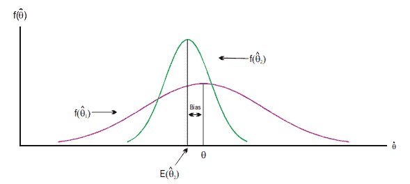
Suppose we are given two estimators $\widehat{\theta}_1$ and $\widehat{\theta}_2$ of $\theta$ where the first is unbiased and has a large variance and the second is biased but with a small variance. The question is which one of these two estimators is preferable? $\widehat{\theta}_1$ is unbiased whereas $\widehat{\theta}_2$ is biased. This means that if we repeat the sampling procedure many times, then we expect $\widehat{\theta}_1$ to be on the average correct, whereas $\widehat{\theta}_2$ would be on the average different from $\theta$. However, in real life, we observe only one sample. With a large variance for $\widehat{\theta}_1$, there is a great likelihood that the sample drawn could result in a $\widehat{\theta}_1$ far away from $\theta$. However, with a small variance for $\widehat{\theta}_2$, there is a better chance of getting a $\widehat{\theta}_2$ close to $\theta$. If our loss function is quadratic so that we are penalized when $\widehat{\theta}$ is different from $\theta$ by $L(\widehat{\theta}, \theta)=(\widehat{\theta}-\theta)^2$, then our risk is
$$
\begin{aligned}
R(\widehat{\theta}, \theta) &=E[L(\widehat{\theta}, \theta)]=E(\widehat{\theta}-\theta)^2=M S E(\widehat{\theta}) \
&=E[\widehat{\theta}-E(\widehat{\theta})+E(\widehat{\theta})-\theta]^2=\operatorname{var}(\widehat{\theta})+(\operatorname{Bias}(\widehat{\theta}))^2 .
\end{aligned}
$$
Minimizing the risk when the loss function is quadratic is equivalent to minimizing the Mean Square Error (MSE). From its definition the MSE shows the trade-off between bias and variance. MVU theory sets the bias equal to zero and minimizes $\operatorname{var}(\widehat{\theta})$. In other words, it minimizes the above risk function but only over $\widehat{\theta}$ ‘s that are unbiased. If we do not restrict ourselves to unbiased estimators of $\theta$, minimizing MSE may result in a biased estimator such as $\widehat{\theta}_2$ which beats $\widehat{\theta}_1$ because the gain from its smaller variance outweighs the loss from its small bias, see Fig. 2.2.
经济代写|计量经济学代写Econometrics代考|Hypothesis Testing
The best way to proceed is with an example.
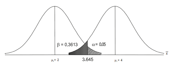
Example 2.10. The Economics Departments instituted a new program to teach micro-principles. We would like to test the null hypothesis that $80 \%$ of economics undergraduate students will pass the micro-principles course versus the alternative hypothesis that only $50 \%$ will pass. We draw a random sample of size 20 from the large undergraduate micro-principles class, and as a simple rule we accept the null if $x$, the number of passing students is larger or equal to 13 , otherwise the alternative hypothesis will be accepted. Note that the distribution we are drawing from is Bernoulli with the probability of success $\theta$, and we have chosen only two states of the world $H_0 ; \theta_0=0.80$ and $H_1 ; \theta_1=0.5$. This situation is known as testing a simple hypothesis versus another simple hypothesis because the distribution is completely specified under the null $H_0$ or the alternative hypothesis $H_1$. One would expect $\left(E(x)=n \theta_0\right) 16$ students under $H_0$ and $\left(n \theta_1\right) 10$ students under $H_1$ to pass the micro-principles exams. It seems then logical to take $x \geq 13$ as the cutoff point distinguishing $H_0$ from $H_1$. No theoretical justification is given at this stage to this arbitrary choice except to say that it is the mid-point of $\lfloor 10,16]$. Figure $2.3$ shows that one can make two types of errors. The first is rejecting $H_0$ when in fact it is true; this is known as type I error and the probability of committing this error is denoted by $\alpha$. The second is accepting $H_0$ when it is false. This is known as type II error, and the corresponding probability is denoted by $\beta$. For this example
$$
\begin{aligned}
\alpha &=\operatorname{Pr}\left[\text { rejecting } H_0 / H_0 \text { is true }\right]=\operatorname{Pr}[x<13 / \theta=0.8] \
&=b(n=20 ; x=0 ; \theta=0.8)+. .+b(n=20 ; x=12 ; \theta=0.8) \
&=b(n=20 ; x=20 ; \theta=0.2)+. .+b(n=20 ; x=8 ; \theta=0.2) \
&=0+. .+0+0.0001+0.0005+0.0020+0.0074+0.0222=0.0322
\end{aligned}
$$
where we have used the fact that $b(n ; x ; \theta)=b(n ; n-x ; 1-\theta)$ and $b(n ; x ; \theta)=$ $\left(\begin{array}{l}n \ x\end{array}\right) \theta^x(1-\theta)^{n-x}$ denotes the binomial distribution for $x=0,1, \ldots, n$, see Problem 4.
$$
\begin{aligned}
\beta &=\operatorname{Pr}\left[\text { accepting } H_0 / H_0 \text { is false }\right]=\operatorname{Pr}[x \geq 13 / \theta=0.5] \
&=b(n=20 ; x=13 ; \theta=0.5)+. .+b(n=20 ; x=20 ; \theta=0.5) \
&=0.0739+0.0370+0.0148+0.0046+0.0011+0.0002+0+0=0.1316
\end{aligned}
$$
计量经济学代考
经济代写|计量经济学代写Econometrics代考|Comparing Biased and Unbiased Estimators
假设我们有两个估计量 $\hat{\theta}_1$ 和 $\hat{\theta}_2$ 的 $\theta$ 其中第一个是无偏的并且方差很大,第二个是有偏的但方差很小。问题是这 两个估计器中哪一个更可取? $\hat{\theta}_1$ 是无偏见的,而 $\hat{\theta}_2$ 是有偏见的。这意味着如果我们多次重复采样过程,那么我 们期望 $\hat{\theta}_1$ 平均来说是正确的,而 $\hat{\theta}_2$ 平均而言不同于 $\theta$. 然而,在现实生活中,我们只观察到一个样本。有很大的 差异 $\hat{\theta}_1$ ,抽取的样本很可能会导致 $\hat{\theta}_1$ 远离 $\theta$. 然而,对于 $\hat{\theta}_2$, 有更好的机会获得 $\hat{\theta}_2$ 相近 $\theta$. 如果我们的损失函数是 二次的,那么我们会受到惩罚 $\hat{\theta}$ 不同于 $\theta$ 经过 $L(\hat{\theta}, \theta)=(\hat{\theta}-\theta)^2$ ,那么我们的风险是
$$
R(\hat{\theta}, \theta)=E[L(\hat{\theta}, \theta)]=E(\hat{\theta}-\theta)^2=M S E(\hat{\theta}) \quad=E[\hat{\theta}-E(\hat{\theta})+E(\hat{\theta})-\theta]^2=\operatorname{var}(\hat{\theta})+(\operatorname{Bias}
$$
当损失函数是二次函数时最小化风险等同于最小化均方误差 (MSE)。根据其定义,MSE 显示了偏差和方差之间 的权衡。MVU 理论将偏差设置为零并最小化 $\operatorname{var}(\hat{\theta})$. 换句话说,它最小化了上述风险函数,但仅超过 $\hat{\theta}$ 这是公 正的。如果我们不限制自己的无偏估计量 $\theta$ ,最小化 MSE 可能会导致有偏差的估计,例如 $\hat{\theta}_2$ 哪个节拍 $\hat{\theta}_1$ 因为它 较小的方差带来的收益超过了它的小偏差带来的损失,见图 2.2。
经济代写|计量经济学代写Econometrics代考|Hypothesis Testing
最好的方法是举个例子。
示例 2.10。经济系制定了一项新计划来教授微观原理。我们想检验零假设 $80 \%$ 的经济学本科生将通过微观原理 课程,而备择假设只有 $50 \%$ 将通过。我们从大型本科溦观原理课程中随机抽取 20 个样本,作为一个简单的规 则,如果 $x$ ,通过学生的人数大于或等于 13 ,否则将接受备择假设。请注意,我们从中得出的分布是具有成功概 率的伯努利分布 $\theta$, 我们只选择了世界上的两个状态 $H_0 ; \theta_0=0.80$ 和 $H_1 ; \theta_1=0.5$. 这种情况被称为检验一个 简单假设与另一个简单假设,因为分布完全在 null 下指定 $H_0$ 或替代假设 $H_1$. 人们会期望 $\left(E(x)=n \theta_0\right) 16$ 下 的学生 $H_0$ 和 $\left(n \theta_1\right) 10$ 下的学生 $H_1$ 通过微观原理考试。这似乎是合乎逻辑的 $x \geq 13$ 作为分界点 $H_0$ 从 $H_1$. 在这 个阶段没有对这个任意选择给出理论依据,只是说它是 $\lfloor 10,16]$. 数字 $2.3$ 表明一个人可以犯两种类型的错误。第 一个是拒绝 $H_0$ 事实上它是真的;这称为 I 类错误,犯此错误的概率表示为 $\alpha$. 第二个是接受 $H_0$ 当它是假的。这 被称为 II 类错误,相应的概率表示为 $\beta$. 对于这个例子
$\alpha=\operatorname{Pr}\left[\right.$ rejecting $H_0 / H_0$ is true $]=\operatorname{Pr}[x<13 / \theta=0.8] \quad=b(n=20 ; x=0 ; \theta=0.8)+\ldots+b(n$
我们在哪里使用了这个事实 $b(n ; x ; \theta)=b(n ; n-x ; 1-\theta)$ 和 $b(n ; x ; \theta)=(n x) \theta^x(1-\theta)^{n-x}$ 表示二项 分布 $x=0,1, \ldots, n$ ,见问题 4 。
$\beta=\operatorname{Pr}\left[\right.$ accepting $H_0 / H_0$ is false $]=\operatorname{Pr}[x \geq 13 / \theta=0.5] \quad=b(n=20 ; x=13 ; \theta=0.5)+\ldots+b$

统计代写请认准statistics-lab™. statistics-lab™为您的留学生涯保驾护航。
金融工程代写
金融工程是使用数学技术来解决金融问题。金融工程使用计算机科学、统计学、经济学和应用数学领域的工具和知识来解决当前的金融问题,以及设计新的和创新的金融产品。
非参数统计代写
非参数统计指的是一种统计方法,其中不假设数据来自于由少数参数决定的规定模型;这种模型的例子包括正态分布模型和线性回归模型。
广义线性模型代考
广义线性模型(GLM)归属统计学领域,是一种应用灵活的线性回归模型。该模型允许因变量的偏差分布有除了正态分布之外的其它分布。
术语 广义线性模型(GLM)通常是指给定连续和/或分类预测因素的连续响应变量的常规线性回归模型。它包括多元线性回归,以及方差分析和方差分析(仅含固定效应)。
有限元方法代写
有限元方法(FEM)是一种流行的方法,用于数值解决工程和数学建模中出现的微分方程。典型的问题领域包括结构分析、传热、流体流动、质量运输和电磁势等传统领域。
有限元是一种通用的数值方法,用于解决两个或三个空间变量的偏微分方程(即一些边界值问题)。为了解决一个问题,有限元将一个大系统细分为更小、更简单的部分,称为有限元。这是通过在空间维度上的特定空间离散化来实现的,它是通过构建对象的网格来实现的:用于求解的数值域,它有有限数量的点。边界值问题的有限元方法表述最终导致一个代数方程组。该方法在域上对未知函数进行逼近。[1] 然后将模拟这些有限元的简单方程组合成一个更大的方程系统,以模拟整个问题。然后,有限元通过变化微积分使相关的误差函数最小化来逼近一个解决方案。
tatistics-lab作为专业的留学生服务机构,多年来已为美国、英国、加拿大、澳洲等留学热门地的学生提供专业的学术服务,包括但不限于Essay代写,Assignment代写,Dissertation代写,Report代写,小组作业代写,Proposal代写,Paper代写,Presentation代写,计算机作业代写,论文修改和润色,网课代做,exam代考等等。写作范围涵盖高中,本科,研究生等海外留学全阶段,辐射金融,经济学,会计学,审计学,管理学等全球99%专业科目。写作团队既有专业英语母语作者,也有海外名校硕博留学生,每位写作老师都拥有过硬的语言能力,专业的学科背景和学术写作经验。我们承诺100%原创,100%专业,100%准时,100%满意。
随机分析代写
随机微积分是数学的一个分支,对随机过程进行操作。它允许为随机过程的积分定义一个关于随机过程的一致的积分理论。这个领域是由日本数学家伊藤清在第二次世界大战期间创建并开始的。
时间序列分析代写
随机过程,是依赖于参数的一组随机变量的全体,参数通常是时间。 随机变量是随机现象的数量表现,其时间序列是一组按照时间发生先后顺序进行排列的数据点序列。通常一组时间序列的时间间隔为一恒定值(如1秒,5分钟,12小时,7天,1年),因此时间序列可以作为离散时间数据进行分析处理。研究时间序列数据的意义在于现实中,往往需要研究某个事物其随时间发展变化的规律。这就需要通过研究该事物过去发展的历史记录,以得到其自身发展的规律。
回归分析代写
多元回归分析渐进(Multiple Regression Analysis Asymptotics)属于计量经济学领域,主要是一种数学上的统计分析方法,可以分析复杂情况下各影响因素的数学关系,在自然科学、社会和经济学等多个领域内应用广泛。
MATLAB代写
MATLAB 是一种用于技术计算的高性能语言。它将计算、可视化和编程集成在一个易于使用的环境中,其中问题和解决方案以熟悉的数学符号表示。典型用途包括:数学和计算算法开发建模、仿真和原型制作数据分析、探索和可视化科学和工程图形应用程序开发,包括图形用户界面构建MATLAB 是一个交互式系统,其基本数据元素是一个不需要维度的数组。这使您可以解决许多技术计算问题,尤其是那些具有矩阵和向量公式的问题,而只需用 C 或 Fortran 等标量非交互式语言编写程序所需的时间的一小部分。MATLAB 名称代表矩阵实验室。MATLAB 最初的编写目的是提供对由 LINPACK 和 EISPACK 项目开发的矩阵软件的轻松访问,这两个项目共同代表了矩阵计算软件的最新技术。MATLAB 经过多年的发展,得到了许多用户的投入。在大学环境中,它是数学、工程和科学入门和高级课程的标准教学工具。在工业领域,MATLAB 是高效研究、开发和分析的首选工具。MATLAB 具有一系列称为工具箱的特定于应用程序的解决方案。对于大多数 MATLAB 用户来说非常重要,工具箱允许您学习和应用专业技术。工具箱是 MATLAB 函数(M 文件)的综合集合,可扩展 MATLAB 环境以解决特定类别的问题。可用工具箱的领域包括信号处理、控制系统、神经网络、模糊逻辑、小波、仿真等。