如果你也在 怎样代写代数学Algebra这个学科遇到相关的难题,请随时右上角联系我们的24/7代写客服。
现代代数是数学的一个分支,涉及各种集合(如实数、复数、矩阵和矢量空间)的一般代数结构,而不是操作其个别元素的规则和程序。
statistics-lab™ 为您的留学生涯保驾护航 在代写代数学Algebra方面已经树立了自己的口碑, 保证靠谱, 高质且原创的统计Statistics代写服务。我们的专家在代写代数学Algebra代写方面经验极为丰富,各种代写代数学Algebra相关的作业也就用不着说。
我们提供的代数学Algebra及其相关学科的代写,服务范围广, 其中包括但不限于:
- Statistical Inference 统计推断
- Statistical Computing 统计计算
- Advanced Probability Theory 高等概率论
- Advanced Mathematical Statistics 高等数理统计学
- (Generalized) Linear Models 广义线性模型
- Statistical Machine Learning 统计机器学习
- Longitudinal Data Analysis 纵向数据分析
- Foundations of Data Science 数据科学基础
数学代写|代数学代写Algebra代考|Scalar Multiplication
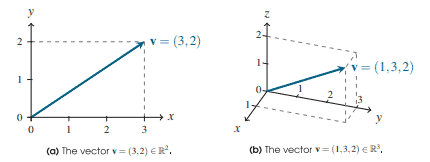
The other basic operation on vectors that we introduce at this point is one that changes a vector’s length and/or reverses its direction, but does not otherwise change the direction in which it points.
Suppose $\mathbf{v}=\left(v_1, v_2, \ldots, v_n\right) \in \mathbb{R}^n$ is a vector and $c \in \mathbb{R}$ is a scalar. Then their scalar multiplication, denoted by $c \mathbf{v}$, is the vector
$$
c \mathbf{v} \stackrel{\text { dff }}{=}\left(c v_1, c v_2, \ldots, c v_n\right) .
$$
We remark that, once again, algebraically this is exactly the definition that someone would likely expect the quantity $c \mathbf{v}$ to have. Multiplying each entry of $\mathbf{v}$ by $c$ seems like a rather natural operation, and it has the simple geometric interpretation of stretching $\mathbf{v}$ by a factor of $c$, as in Figure 1.4. In particular, if $|c|>1$ then scalar multiplication stretches $\mathbf{v}$, but if $|c|<1$ then it shrinks $\mathbf{v}$. When $c<0$ then this operation also reverses the direction of $\mathbf{v}$, in addition to any stretching or shrinking that it does if $|c| \neq 1$.
Two special cases of scalar multiplication are worth pointing out:
- If $c=0$ then $c v$ is the zero vector, all of whose entries are 0 , which we denote by 0 .
- If $c=-1$ then $c \mathbf{v}$ is the vector whose entries are the negatives of $\mathbf{v}$ ‘s entries, which we denote by $-\mathbf{v}$.
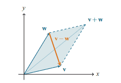
We also define vector subtraction via $\mathbf{v}-\mathbf{w} \stackrel{\text { dif }}{=} \mathbf{v}+(-\mathbf{w})$, and we note that it has the geometric interpretation that $\mathbf{v}-\mathbf{w}$ is the vector pointing from the head of $\mathbf{w}$ to the head of $\mathbf{v}$ when $\mathbf{v}$ and $\mathbf{w}$ are in standard position. It is perhaps easiest to keep this geometric picture straight (“it points from the head of which vector to the head of the other one?”) if we just think of $\mathbf{v}-\mathbf{w}$ as the vector that must be added to $\mathbf{w}$ to get $\mathbf{v}$ (so it points from $\mathbf{w}$ to $\mathbf{v}$ ). Alternatively, $\mathbf{v}-\mathbf{w}$ is the other diagonal (besides $\mathbf{v}+\mathbf{w}$ ) in the parallelogram with sides $\mathbf{v}$ and $\mathbf{w}$, as in Figure 1.5. - It is straightforward to verify some simple properties of the zero vector, such as the facts that $\mathbf{v}-\mathbf{v}=\mathbf{0}$ and $\mathbf{v}+\mathbf{0}=\mathbf{v}$ for every vector $\mathbf{v} \in \mathbb{R}^n$, by working entry-by-entry with the vector operations. There are also quite a few other simple ways in which scalar multiplication interacts with vector addition, some of which we now list explicitly for easy reference.
数学代写|代数学代写Algebra代考|Linear Combinations
One common task in linear algebra is to start out with some given collection of vectors $\mathbf{v}_1, \mathbf{v}_2, \ldots, \mathbf{v}_k$ and then use vector addition and scalar multiplication to construct new vectors out of them. The following definition gives a name to this concept.
For example, $(1,2,3)$ is a linear combination of the vectors $(1,1,1)$ and $(-1,0,1)$ since $(1,2,3)=2(1,1,1)+(-1,0,1)$. On the other hand, $(1,2,3)$ is not a linear combination of the vectors $(1,1,0)$ and $(2,1,0)$ since every vector of the form $c_1(1,1,0)+c_2(2,1,0)$ has a 0 in its third entry, and thus cannot possibly equal $(1,2,3)$.
When working with linear combinations, some particularly important vectors are those with all entries equal to 0 , except for a single entry that equals 1 . Specifically, for each $j=1,2, \ldots, n$, we define the vector $\mathbf{e}_j \in \mathbb{R}^n$ by
$$
\mathbf{e}_j \stackrel{\text { df }}{=}(0,0, \ldots, 0,1,0, \ldots, 0) .
$$
For example, in $\mathbb{R}^2$ there are two such vectors: $\mathbf{e}_1=(1,0)$ and $\mathbf{e}_2=(0,1)$. Similarly, in $\mathbb{R}^3$ there are three such vectors: $\mathbf{e}_1=(1,0,0), \mathbf{e}_2=(0,1,0)$, and $\mathbf{e}_3=(0,0,1)$. In general, in $\mathbb{R}^n$ there are $n$ of these vectors, $\mathbf{e}_1, \mathbf{e}_2, \ldots, \mathbf{e}_n$, and we call them the standard basis vectors (for reasons that we discuss in the next chapter). Notice that in $\mathbb{R}^2$ and $\mathbb{R}^3$, these are the vectors that point a distance of 1 in the direction of the $x-, y$-, and $z$-axes, as in Figure 1.6.
For now, the reason for our interest in these standard basis vectors is that every vector $\mathbf{v} \in \mathbb{R}^n$ can be written as a linear combination of them. In particular, if $\mathbf{v}=\left(v_1, v_2, \ldots, v_n\right)$ then
$$
\mathbf{v}=v_1 \mathbf{e}_1+v_2 \mathbf{e}_2+\cdots+v_n \mathbf{e}_n,
$$
which can be verified just by computing each of the entries of the linear combination on the right. This idea of writing vectors in terms of the standard basis vectors (or other distinguished sets of vectors that we introduce later) is one of the most useful techniques that we make use of in linear algebra: in many situations, if we can prove that some property holds for the standard basis vectors, then we can use linear combinations to show that it must hold for all vectors.
代数学代考
数学代写|代数学代写Algebra代考|标量乘法
我们在这里介绍的另一个关于向量的基本操作是改变向量的长度和/或反转它的方向,但不改变它所指向的方向
假设 $\mathbf{v}=\left(v_1, v_2, \ldots, v_n\right) \in \mathbb{R}^n$ 是一个向量 $c \in \mathbb{R}$ 是一个标量。然后是它们的标量乘法,用 $c \mathbf{v}$,是向量
$$
c \mathbf{v} \stackrel{\text { dff }}{=}\left(c v_1, c v_2, \ldots, c v_n\right) .
$$我们注意到,再一次,从代数上讲,这正是某人可能期望的量的定义 $c \mathbf{v}$ 拥有。乘以的每一项 $\mathbf{v}$ 通过 $c$ 看起来是一个很自然的操作,它对拉伸有简单的几何解释 $\mathbf{v}$ 乘以 $c$,如图1.4所示。特别是,如果 $|c|>1$ 那么标量乘法就会延伸 $\mathbf{v}$,但如果 $|c|<1$ 然后收缩 $\mathbf{v}$。什么时候 $c<0$ 那么这个操作的方向也就颠倒了 $\mathbf{v}$除了它所做的任何拉伸或收缩 $|c| \neq 1$.
标量乘法的两个特殊情况值得指出:
- $c=0$ 然后 $c v$ 是零向量,它的所有元素都是0,我们用0表示。
- If $c=-1$ 然后 $c \mathbf{v}$ 这个向量的分量是负数吗 $\mathbf{v}$ 的条目,我们用 $-\mathbf{v}$.
我们还通过定义向量减法 $\mathbf{v}-\mathbf{w} \stackrel{\text { dif }}{=} \mathbf{v}+(-\mathbf{w})$,我们注意到它的几何解释是 $\mathbf{v}-\mathbf{w}$ 向量是否指向的头部 $\mathbf{w}$ 到 $\mathbf{v}$ 何时 $\mathbf{v}$ 和 $\mathbf{w}$ 处于标准位置。也许最容易保持这个几何图形的直线(“它从哪个向量的头部指向另一个向量的头部?”),如果我们只是想 $\mathbf{v}-\mathbf{w}$ 作为必须加到的向量 $\mathbf{w}$ 得到 $\mathbf{v}$ (所以它指向 $\mathbf{w}$ 到 $\mathbf{v}$ )。或者, $\mathbf{v}-\mathbf{w}$ 另一条对角线(除了? $\mathbf{v}+\mathbf{w}$ )在有边的平行四边形中 $\mathbf{v}$ 和 $\mathbf{w}$,如图1.5所示。 - 验证零向量的一些简单性质是很直接的,比如 $\mathbf{v}-\mathbf{v}=\mathbf{0}$ 和 $\mathbf{v}+\mathbf{0}=\mathbf{v}$ 对于每一个向量 $\mathbf{v} \in \mathbb{R}^n$,通过用向量运算进行逐入口运算。还有许多其他简单的方法可以使标量乘法与向量加法相互作用,我们现在显式列出其中一些方法,以方便参考
数学代写|代数学代写Algebra代考|线性组合
线性代数中的一个常见任务是,从某个给定的向量集合$\mathbf{v}_1, \mathbf{v}_2, \ldots, \mathbf{v}_k$开始,然后使用向量加法和标量乘法从它们中构造出新的向量。下面的定义给出了这个概念的名称例如,$(1,2,3)$是由$(1,2,3)=2(1,1,1)+(-1,0,1)$开始的向量$(1,1,1)$和$(-1,0,1)$的线性组合。另一方面,$(1,2,3)$不是向量$(1,1,0)$和$(2,1,0)$的线性组合,因为$c_1(1,1,0)+c_2(2,1,0)$形式的每个向量在第三个条目中都有一个0,因此不可能等于$(1,2,3)$当处理线性组合时,一些特别重要的向量是那些所有项都等于0的向量,只有一个项等于1。具体来说,对于每个$j=1,2, \ldots, n$,我们通过
$$
\mathbf{e}_j \stackrel{\text { df }}{=}(0,0, \ldots, 0,1,0, \ldots, 0) .
$$
来定义向量$\mathbf{e}_j \in \mathbb{R}^n$。例如,在$\mathbb{R}^2$中有两个这样的向量:$\mathbf{e}_1=(1,0)$和$\mathbf{e}_2=(0,1)$。类似地,在$\mathbb{R}^3$中有三个这样的向量:$\mathbf{e}_1=(1,0,0), \mathbf{e}_2=(0,1,0)$和$\mathbf{e}_3=(0,0,1)$。一般来说,在$\mathbb{R}^n$中有$n$这些向量,$\mathbf{e}_1, \mathbf{e}_2, \ldots, \mathbf{e}_n$,我们称它们为标准基向量(原因我们将在下一章讨论)。注意,在$\mathbb{R}^2$和$\mathbb{R}^3$中,这些是指向$x-, y$ -和$z$ -轴方向上距离为1的向量,如图1.6所示现在,我们对这些标准基向量感兴趣的原因是,每个向量$\mathbf{v} \in \mathbb{R}^n$都可以写成它们的线性组合。特别是,如果$\mathbf{v}=\left(v_1, v_2, \ldots, v_n\right)$那么
$$
\mathbf{v}=v_1 \mathbf{e}_1+v_2 \mathbf{e}_2+\cdots+v_n \mathbf{e}_n,
$$
这可以通过计算右边线性组合的每一项来验证。这种用标准基向量(或我们稍后介绍的其他不同的向量集)来表示向量的想法是我们在线性代数中使用的最有用的技巧之一:在许多情况下,如果我们能证明某些性质适用于标准基向量,那么我们就可以使用线性组合来证明它一定适用于所有向量

统计代写请认准statistics-lab™. statistics-lab™为您的留学生涯保驾护航。
金融工程代写
金融工程是使用数学技术来解决金融问题。金融工程使用计算机科学、统计学、经济学和应用数学领域的工具和知识来解决当前的金融问题,以及设计新的和创新的金融产品。
非参数统计代写
非参数统计指的是一种统计方法,其中不假设数据来自于由少数参数决定的规定模型;这种模型的例子包括正态分布模型和线性回归模型。
广义线性模型代考
广义线性模型(GLM)归属统计学领域,是一种应用灵活的线性回归模型。该模型允许因变量的偏差分布有除了正态分布之外的其它分布。
术语 广义线性模型(GLM)通常是指给定连续和/或分类预测因素的连续响应变量的常规线性回归模型。它包括多元线性回归,以及方差分析和方差分析(仅含固定效应)。
有限元方法代写
有限元方法(FEM)是一种流行的方法,用于数值解决工程和数学建模中出现的微分方程。典型的问题领域包括结构分析、传热、流体流动、质量运输和电磁势等传统领域。
有限元是一种通用的数值方法,用于解决两个或三个空间变量的偏微分方程(即一些边界值问题)。为了解决一个问题,有限元将一个大系统细分为更小、更简单的部分,称为有限元。这是通过在空间维度上的特定空间离散化来实现的,它是通过构建对象的网格来实现的:用于求解的数值域,它有有限数量的点。边界值问题的有限元方法表述最终导致一个代数方程组。该方法在域上对未知函数进行逼近。[1] 然后将模拟这些有限元的简单方程组合成一个更大的方程系统,以模拟整个问题。然后,有限元通过变化微积分使相关的误差函数最小化来逼近一个解决方案。
tatistics-lab作为专业的留学生服务机构,多年来已为美国、英国、加拿大、澳洲等留学热门地的学生提供专业的学术服务,包括但不限于Essay代写,Assignment代写,Dissertation代写,Report代写,小组作业代写,Proposal代写,Paper代写,Presentation代写,计算机作业代写,论文修改和润色,网课代做,exam代考等等。写作范围涵盖高中,本科,研究生等海外留学全阶段,辐射金融,经济学,会计学,审计学,管理学等全球99%专业科目。写作团队既有专业英语母语作者,也有海外名校硕博留学生,每位写作老师都拥有过硬的语言能力,专业的学科背景和学术写作经验。我们承诺100%原创,100%专业,100%准时,100%满意。
随机分析代写
随机微积分是数学的一个分支,对随机过程进行操作。它允许为随机过程的积分定义一个关于随机过程的一致的积分理论。这个领域是由日本数学家伊藤清在第二次世界大战期间创建并开始的。
时间序列分析代写
随机过程,是依赖于参数的一组随机变量的全体,参数通常是时间。 随机变量是随机现象的数量表现,其时间序列是一组按照时间发生先后顺序进行排列的数据点序列。通常一组时间序列的时间间隔为一恒定值(如1秒,5分钟,12小时,7天,1年),因此时间序列可以作为离散时间数据进行分析处理。研究时间序列数据的意义在于现实中,往往需要研究某个事物其随时间发展变化的规律。这就需要通过研究该事物过去发展的历史记录,以得到其自身发展的规律。
回归分析代写
多元回归分析渐进(Multiple Regression Analysis Asymptotics)属于计量经济学领域,主要是一种数学上的统计分析方法,可以分析复杂情况下各影响因素的数学关系,在自然科学、社会和经济学等多个领域内应用广泛。
MATLAB代写
MATLAB 是一种用于技术计算的高性能语言。它将计算、可视化和编程集成在一个易于使用的环境中,其中问题和解决方案以熟悉的数学符号表示。典型用途包括:数学和计算算法开发建模、仿真和原型制作数据分析、探索和可视化科学和工程图形应用程序开发,包括图形用户界面构建MATLAB 是一个交互式系统,其基本数据元素是一个不需要维度的数组。这使您可以解决许多技术计算问题,尤其是那些具有矩阵和向量公式的问题,而只需用 C 或 Fortran 等标量非交互式语言编写程序所需的时间的一小部分。MATLAB 名称代表矩阵实验室。MATLAB 最初的编写目的是提供对由 LINPACK 和 EISPACK 项目开发的矩阵软件的轻松访问,这两个项目共同代表了矩阵计算软件的最新技术。MATLAB 经过多年的发展,得到了许多用户的投入。在大学环境中,它是数学、工程和科学入门和高级课程的标准教学工具。在工业领域,MATLAB 是高效研究、开发和分析的首选工具。MATLAB 具有一系列称为工具箱的特定于应用程序的解决方案。对于大多数 MATLAB 用户来说非常重要,工具箱允许您学习和应用专业技术。工具箱是 MATLAB 函数(M 文件)的综合集合,可扩展 MATLAB 环境以解决特定类别的问题。可用工具箱的领域包括信号处理、控制系统、神经网络、模糊逻辑、小波、仿真等。