cs代写|复杂网络代写complex network代考|CS60078
如果你也在 怎样代写复杂网络complex network这个学科遇到相关的难题,请随时右上角联系我们的24/7代写客服。
在网络理论的背景下,复杂网络是具有非微观拓扑特征的图(网络)这些特征在格子或随机图等简单网络中不出现,但在代表真实系统的网络中经常出现。
statistics-lab™ 为您的留学生涯保驾护航 在代写复杂网络complex network方面已经树立了自己的口碑, 保证靠谱, 高质且原创的统计Statistics代写服务。我们的专家在代写复杂网络complex network代写方面经验极为丰富,各种代写复杂网络complex network相关的作业也就用不着说。
我们提供的复杂网络complex network及其相关学科的代写,服务范围广, 其中包括但不限于:
- Statistical Inference 统计推断
- Statistical Computing 统计计算
- Advanced Probability Theory 高等概率论
- Advanced Mathematical Statistics 高等数理统计学
- (Generalized) Linear Models 广义线性模型
- Statistical Machine Learning 统计机器学习
- Longitudinal Data Analysis 纵向数据分析
- Foundations of Data Science 数据科学基础
cs代写|复杂网络代写complex network代考|COMPLEX NETWORK SYSTEMS
Far from being separate entities, many natural, social, and engineering systems can be considered as CNSs associated with tight interactions among neighboring entities within them $[3,10,18,29,39,50,92,120,130,141,175,194,201,211,219]$. Roughly speaking, a CNS refers to a networking system that consists of lots of interconnected agents, where each agent is an elementary element or a fundamental unit with detailed contents depending on the nature of the specific network under consideration [175]. For example, the Internet is a CNS of routers and computers connected by various physical or wireless links. The cell can be described by a CNS of chemicals connected by chemical interactions. The scientific citation network is a CNS of papers and books linked by citations among them. The WeChat social network is a CNS whose agents are users and whose edges represent the relationships among users, to name just a few.
With the aid of coordination with neighboring individuals, a CNS can exhibit fascinating cooperative behaviors far beyond the individuals’ inherent properties. Prototypical cooperative behaviors include synchronization $[38,95,101,177]$, consensus $[76,118,128]$, swarming $[48,115]$, flocking $[117,161]$. In this book, we focus on the CNSs which include complex networks and MASs as special cases. A lot of new research challenges have been raised about understanding the emergence mechanisms responsible for various collective behaviors as well as global statistical properties of CNSs $[3,15,114,178]$. Network science, as a strong interdisciplinary research field, has been established at the first several years of the 21st century [110]. It is increasingly recognized that a detailed study on cooperative dynamics of CNSs would not only help researchers understand the evolution mechanism for macroscopical cooperative behaviors, but also prompt the application of network science to solve various engineering problems, e.g., design of distributed sensor networks [135], formation control of multiple unmanned aerial vehicles [37], distributed localization [89], and load assignment of multiple energy storage units in modern power grid [191].
Among the various cooperative behaviors of CNSs, synchronization of complex networks and consensus of MASs are the most fundamental yet most important ones. Synchronization of complex networks exhibits the cooperative behavior that the states of all entities within these networks achieve an agreement on some quantities of interest. Compared with stability analysis of an isolated control plant, synchronization behavior analysis in CNSs are much more challenging as the synchronization process is determined by the evolution of network topology as well as the inherent dynamics of individual units within these network systems $[96,102,121,198,199]$. As a topic closely related to synchronization of complex networks, the consensus of MASs has recently gained much attention from various research fields, especially the system science, control theory, and electrical engineering communities $[22,65,88,116,128]$. In the remainder of this chapter, we will review some existing results on achieving synchronization of complex networks and consensus of MASs over dynamically changing communication topologies.
cs代写|复杂网络代写complex network代考|DEFINITIONS OF SYNCHRONIZATION AND CONSENSUS
Before moving forward, the definition of consensus of MASs is given. Moreover, the synchronization of complex networks can be defined similarly.
Consider an MAS which consists of $N$ agents. Without loss of generality, we label the $N$ agents as agents $1, \ldots, N$, respectively. The dynamics of agent $i, i=1, \ldots, N$, are represented by
$$
\dot{x}_i(t)=f\left(t, x_i(t), u_i(t)\right),
$$
where $x_i(t) \in \mathbb{R}^n$ and $u_i(t) \in \mathbb{R}^m$ represent, respectively, the state and the control input, $f(\cdot, \cdot \cdot):\left[t_0,+\infty\right) \times \mathbb{R}^n \times \mathbb{R}^m \mapsto \mathbb{R}^n$ represents the nonlinear dynamics of agent i. A particular case is the general linear time-invariant MASs with the dynamics of agent $i$ are described by
$$
\dot{x}_i(t)=A x_i(t)+B u_i(t), i=1, \ldots, N,
$$
where $A \in \mathbb{R}^{n \times n}$ and $B \in \mathbb{R}^{n \times m}$ represent, respectively, the state matrix and control input matrix. For convenience, throughout this book, we call MAS (1.1) to represent the MAS whose dynamics are described by (1.1).
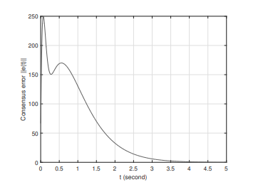
Definition $1.1$ Consensus of the MAS (1.1) is said to be achieved if for arbitrary initial conditions $x_i\left(t_0\right), i=1, \ldots, N$,
$$
\lim _{t \rightarrow \infty}\left|x_i(t)-x_j(t)\right|=0, i, j=1, \ldots, N .
$$
The definition of consensus for MAS (1.1) given by Eq. (1.3) does not concern about the final consensus states. However, it is sometimes important to make the states of all agents in the considered MASs to finally converge to some predesigned trajectory, especially from the viewpoint of controlling various complex engineering systems. To ensure the states of all agents in MAS (1.1) converge to some desired states, a target system (may be virtual) is introduced to the network (1.1) as
$$
\dot{s}(t)=f(t, s(t))
$$
for some given initial value $s\left(t_0\right) \in \mathbb{R}^n$. Under this scenario, we call agent $i$ whose dynamics are described by (1.1) the follower $i, i=1, \ldots, N$, and call the agent whose dynamics are described by (1.4) the leader.
复杂网络代写
cs代写|复杂网络代写complex network代考|COMPLEX NETWORK SYSTEMS
许多自然、社会和工程系统远不是独立的实体,而是可以被视为与其中相邻实体之间紧密相互作用相关的 CNS[3,10,18,29,39,50,92,120,130,141,175,194,201,211,219]. 粗略地说,CNS 是指由许多相互连接的代理组成的网络系统,其中每个代理是一个基本元素或基本单元,其详细内容取决于所考虑的特定网络的性质[175]。例如,互联网是通过各种物理或无线链路连接的路由器和计算机的 CNS。细胞可以通过化学相互作用连接的化学中枢神经系统来描述。科学引文网络是论文和书籍之间通过引文链接的 CNS。微信社交网络是一个CNS,其代理是用户,其边代表用户之间的关系,仅举几例。
借助与邻近个体的协调,CNS 可以表现出远远超出个体固有属性的迷人合作行为。典型的合作行为包括同步[38,95,101,177], 共识[76,118,128], 蜂拥而至[48,115], 植绒[117,161]. 在本书中,我们重点关注包含复杂网络和 MAS 的 CNS 作为特例。关于理解负责各种集体行为的出现机制以及 CNS 的全局统计特性,已经提出了许多新的研究挑战[3,15,114,178]. 网络科学作为一个强大的跨学科研究领域,在 21 世纪头几年已经确立[110]。人们越来越认识到,对 CNS 合作动力学的详细研究不仅有助于研究人员了解宏观合作行为的演化机制,而且还促进网络科学应用于解决各种工程问题,例如分布式传感器网络的设计 [135 ],多架无人机编队控制[37],分布式定位[89],现代电网中多个储能单元的负荷分配[191]。
在 CNS 的各种协作行为中,复杂网络的同步和 MAS 的共识是最基本也是最重要的。复杂网络的同步展示了这些网络中所有实体的状态就某些感兴趣的数量达成一致的合作行为。与孤立控制设备的稳定性分析相比,CNS 中的同步行为分析更具挑战性,因为同步过程取决于网络拓扑的演变以及这些网络系统中各个单元的固有动态[96,102,121,198,199]. 作为与复杂网络同步密切相关的课题,MASs 的共识最近引起了各个研究领域的广泛关注,尤其是系统科学、控制理论和电气工程界。[22,65,88,116,128]. 在本章的剩余部分,我们将回顾一些关于实现复杂网络同步和 MAS 在动态变化的通信拓扑上的共识的现有结果。
cs代写|复杂网络代写complex network代考|DEFINITIONS OF SYNCHRONIZATION AND CONSENSUS
在继续之前,给出了MAS共识的定义。此外,可以类似地定义复杂网络的同步。
考虑一个 MAS,它由 $N$ 代理。不失一般性,我们标记 $N$ 代理人作为代理人 $1, \ldots, N$ ,分别。代理的动态 $i, i=1, \ldots, N$, 表示为
$$
\dot{x}i(t)=f\left(t, x_i(t), u_i(t)\right), $$ 在哪里 $x_i(t) \in \mathbb{R}^n$ 和 $u_i(t) \in \mathbb{R}^m$ 分别表示状态和控制输入, $f(\cdot, \cdot):\left[t_0,+\infty\right) \times \mathbb{R}^n \times \mathbb{R}^m \mapsto \mathbb{R}^n$ 表示代 理 $i$ 的非线性动力学。一个特例是具有代理动力学的一般线性时不变 MAS $i$ 被描述为 $$ \dot{x}_i(t)=A x_i(t)+B u_i(t), i=1, \ldots, N, $$ 在哪里 $A \in \mathbb{R}^{n \times n}$ 和 $B \in \mathbb{R}^{n \times m}$ 分别表示状态矩阵和控制输入矩阵。为方便起见,在整本书中,我们称 MAS (1.1) 来表示其动力学由 (1.1) 描述的 MAS。 定义 $1.1$ 如果对于任意初始条件,则据说可以实现 MAS (1.1) 的共识 $x_i\left(t_0\right), i=1, \ldots, N$ , $$ \lim {t \rightarrow \infty}\left|x_i(t)-x_j(t)\right|=0, i, j=1, \ldots, N .
$$
由方程式给出的 MAS (1.1) 共识的定义。(1.3) 不关心最终共识状态。然而,有时重要的是使所考虑的 MAS 中的所 有代理的状态最终收敛到某个预先设计的轨迹,特别是从控制各种复杂工程系统的角度来看。为了确保 MAS (1.1) 中所有代理的状态收敛到一些期望的状态,将目标系统(可能是虚拟的) 引入网络 (1.1) 为
$$
\dot{s}(t)=f(t, s(t))
$$
对于一些给定的初始值 $s\left(t_0\right) \in \mathbb{R}^n$. 在这种情况下,我们称代理 $i$ 其动力学由 $(1.1)$ 跟随者描述 $i, i=1, \ldots, N$ ,并调用由 (1.4) 描述动态的智能体为领导者。

统计代写请认准statistics-lab™. statistics-lab™为您的留学生涯保驾护航。
金融工程代写
金融工程是使用数学技术来解决金融问题。金融工程使用计算机科学、统计学、经济学和应用数学领域的工具和知识来解决当前的金融问题,以及设计新的和创新的金融产品。
非参数统计代写
非参数统计指的是一种统计方法,其中不假设数据来自于由少数参数决定的规定模型;这种模型的例子包括正态分布模型和线性回归模型。
广义线性模型代考
广义线性模型(GLM)归属统计学领域,是一种应用灵活的线性回归模型。该模型允许因变量的偏差分布有除了正态分布之外的其它分布。
术语 广义线性模型(GLM)通常是指给定连续和/或分类预测因素的连续响应变量的常规线性回归模型。它包括多元线性回归,以及方差分析和方差分析(仅含固定效应)。
有限元方法代写
有限元方法(FEM)是一种流行的方法,用于数值解决工程和数学建模中出现的微分方程。典型的问题领域包括结构分析、传热、流体流动、质量运输和电磁势等传统领域。
有限元是一种通用的数值方法,用于解决两个或三个空间变量的偏微分方程(即一些边界值问题)。为了解决一个问题,有限元将一个大系统细分为更小、更简单的部分,称为有限元。这是通过在空间维度上的特定空间离散化来实现的,它是通过构建对象的网格来实现的:用于求解的数值域,它有有限数量的点。边界值问题的有限元方法表述最终导致一个代数方程组。该方法在域上对未知函数进行逼近。[1] 然后将模拟这些有限元的简单方程组合成一个更大的方程系统,以模拟整个问题。然后,有限元通过变化微积分使相关的误差函数最小化来逼近一个解决方案。
tatistics-lab作为专业的留学生服务机构,多年来已为美国、英国、加拿大、澳洲等留学热门地的学生提供专业的学术服务,包括但不限于Essay代写,Assignment代写,Dissertation代写,Report代写,小组作业代写,Proposal代写,Paper代写,Presentation代写,计算机作业代写,论文修改和润色,网课代做,exam代考等等。写作范围涵盖高中,本科,研究生等海外留学全阶段,辐射金融,经济学,会计学,审计学,管理学等全球99%专业科目。写作团队既有专业英语母语作者,也有海外名校硕博留学生,每位写作老师都拥有过硬的语言能力,专业的学科背景和学术写作经验。我们承诺100%原创,100%专业,100%准时,100%满意。
随机分析代写
随机微积分是数学的一个分支,对随机过程进行操作。它允许为随机过程的积分定义一个关于随机过程的一致的积分理论。这个领域是由日本数学家伊藤清在第二次世界大战期间创建并开始的。
时间序列分析代写
随机过程,是依赖于参数的一组随机变量的全体,参数通常是时间。 随机变量是随机现象的数量表现,其时间序列是一组按照时间发生先后顺序进行排列的数据点序列。通常一组时间序列的时间间隔为一恒定值(如1秒,5分钟,12小时,7天,1年),因此时间序列可以作为离散时间数据进行分析处理。研究时间序列数据的意义在于现实中,往往需要研究某个事物其随时间发展变化的规律。这就需要通过研究该事物过去发展的历史记录,以得到其自身发展的规律。
回归分析代写
多元回归分析渐进(Multiple Regression Analysis Asymptotics)属于计量经济学领域,主要是一种数学上的统计分析方法,可以分析复杂情况下各影响因素的数学关系,在自然科学、社会和经济学等多个领域内应用广泛。
MATLAB代写
MATLAB 是一种用于技术计算的高性能语言。它将计算、可视化和编程集成在一个易于使用的环境中,其中问题和解决方案以熟悉的数学符号表示。典型用途包括:数学和计算算法开发建模、仿真和原型制作数据分析、探索和可视化科学和工程图形应用程序开发,包括图形用户界面构建MATLAB 是一个交互式系统,其基本数据元素是一个不需要维度的数组。这使您可以解决许多技术计算问题,尤其是那些具有矩阵和向量公式的问题,而只需用 C 或 Fortran 等标量非交互式语言编写程序所需的时间的一小部分。MATLAB 名称代表矩阵实验室。MATLAB 最初的编写目的是提供对由 LINPACK 和 EISPACK 项目开发的矩阵软件的轻松访问,这两个项目共同代表了矩阵计算软件的最新技术。MATLAB 经过多年的发展,得到了许多用户的投入。在大学环境中,它是数学、工程和科学入门和高级课程的标准教学工具。在工业领域,MATLAB 是高效研究、开发和分析的首选工具。MATLAB 具有一系列称为工具箱的特定于应用程序的解决方案。对于大多数 MATLAB 用户来说非常重要,工具箱允许您学习和应用专业技术。工具箱是 MATLAB 函数(M 文件)的综合集合,可扩展 MATLAB 环境以解决特定类别的问题。可用工具箱的领域包括信号处理、控制系统、神经网络、模糊逻辑、小波、仿真等。